Comparison of conventional and advanced physical cleaning methods for BASF inge® Multibore® ultrafiltration membranes in seawater applications focusing on membrane fouling

NG KOK SENG (MIKE)

Bachelor’s in Engineering (Environmental)

July 2017

Comparison of conventional and advanced physical cleaning

methods for BASF inge

Multibore

ultrafiltration membranes in

seawater applications focusing on membrane fouling

Dissertation for obtaining the Master degree in Membrane Engineering Erasmus Mundus Master in Membrane Engineering

Advisor: Mr. Christian Staaks, M.Sc, inge GmbH Co-advisors: Mr. Michael Hoffman, B.Eng, inge GmbH

Dr. Svetlozar Velizarov, FCT-UNL

Jury:

Chair: Dr. Isabel Coelhoso - Universidade Nova de Lisboa Examiners: Dr. Damien Quemrner - Université de Montpellier

Dr. Vlastimil Fíla - University of Chemistry and Technology Prague Dr. João Crespo - Universidade Nova de Lisboa

Comparison of conventional and advanced physical

cleaning methods for BASF inge

Multibore

ultrafiltration membranes in seawater applications

focusing on membrane fouling

NG KOK SENG (MIKE)

Bachelor’s in Engineering (Environmental)

Dissertation presented to Faculdade de Ciências e Tecnologia, Universidade Nova de Lisboa for obtaining the master degree in Membrane Engineering

Dissertation presented to Faculdade de Ciências e Tecnologia, Universidade Nova de Lisboa for obtaining the master degree in Membrane Engineering

Comparison of conventional and advanced physical cleaning methods for BASF inge® Multibore® ultrafiltration membranes in seawater applications focusing on membrane fouling

The EM3E Master is an Education Programme supported by the European Commission, the European Membrane Society (EMS), the European Membrane House (EMH), and a large international network of industrial companies, research centres and universities (http://em3e-4sw.eu/em3e/).

Copyright @ NG KOK SENG (MIKE), FCT/UNL

A Faculdade de Ciências e Tecnologia e a Universidade Nova de Lisboa têm o direito, perpétuo e sem limites geográficos, de arquivar e publicar esta dissertação através de exemplares impressos reproduzidos em papel ou de forma digital, ou por qualquer outro meio conhecido ou que venha a ser inventado, e de a divulgar através de repositórios científicos e de admitir a sua cópia e distribuição com objectivos educacionais ou de investigação, não comerciais, desde que seja dado crédito ao autor e editor.

Projecto financiado com o apoio da Comissão Europeia. A informação contida nesta publicação vincula exclusivamente o autor, não sendo a Comissão responsável pela utilização que dela possa ser feita.

Confidential Clause

This final thesis with the title “Comparison of conventional and advanced physical cleaning methods for BASF inge® Multibore® ultrafiltration membranes in seawater applications focusing on membrane fouling” is based on internal, confidential data and information of the following enterprise:

inge GmbH

Flurstraße 27 86926 Greifenberg

Germany

This work may only be available to the first and second reviewers and authorized members of the board of examiners. Any publication or duplication of this final thesis, even in parts, is prohibited. An inspection of this work by third parties requires the expressed admission of the author and the company.

I The author, Ng Kok Seng (Mike), would like to thank the following whom have made this semester of his Master’s thesis, a memorable learning experience. The author would also like to put forward his appreciation to these individuals for sharing their invaluable experience, knowledge and providing support, encouragement and assistance for his Master’s thesis work.

- To my family, thank you for your unconditional love and support.

- The company, inge GmbH, for giving the author the chance to do a combined summer internship and to write the Master’s thesis.

- Mr. Christian Staaks and Mr. Michael Hoffman, who were the author’s advisor and co-advisor, respectively. They taught the author on technical knowledge and shared their experiences. The author is appreciative of their patient coaching.

- Mrs. Michaela Krug, Mrs. Cornelia Werzinger and Ms. Sointu Parviainen, who guided the author during the two months internship during the summer of 2016. Special thanks to Ms. Sointu Parviainen for helping the author in accommodation matters.

- The process development team in inge GmbH, for providing assistance to and answering the author’s inquiries.

- Dr. Svetlozar Velizarov, the author’s co-advisor from FCT-UNL. Thank you for your advice, guidance and encouragement.

- Professors, lecturers and staff from Université de Montpellier, Université Paul Sabatier, University of Chemistry and Technology Prague, Universidade Nova De Lisboa, for your patience (with my questions), teachings and the effort in helping EM3E students with administration matters.

- Current and ex-internship/Master’s thesis students in inge GmbH who shared their experiences, knowledge and approach to problem solving. The author enjoyed the free-flowing communication. - Lastly, EM3E students from the 5th batch. Thank you for making this journey a memorable experience filled with joy and laughter. The author wishes everyone the best of luck in future, be it in the academics or in the industry.

III Membrane fouling is a major hurdle for ultrafiltration membrane applications. It may increase the operational costs and shorten the lifespan of membrane. Effective and efficient methods are required for its control and minimisation. In this work, the effect of Capillary Drain was investigated with a pilot plant in the Middle East using inge® Dizzer® XL modules with non-treated seawater. Capillary Drain is a novel method proposed by process development team from inge GmbH to improve the cleaning and foulant removal efficiency.

The process was operated at different flux and filtration times to keep the recovery and feed loading constant. Fouling indices developed by A.H. Nguyen [48] (Total Fouling and Hydraulic Irreversible Fouling Index) and the change in permeability were used for comparison of the efficiency of Capillary Drain.

Membrane process performance with and without Capillary Drain were compared. The former resulted in a lower fouling index, indicating that Capillary Drain slowed down the rate of increase in resistance due to fouling. Effect of Capillary Drain was also investigated when it was introduced one filtration cycle after a chemical enhanced backwash (CEB) and in between CEBs. Better results were seen in the latter. At higher operating flux, Capillary Drain also proved to be effective.

The pilot plant experienced a tremendous increase of Trans-Membrane-Pressure when chlorophyll-a concentration reached levels of 4 µg/l. When this happened, Capillary Drain seemed to be able to remove fouling better than CEB alone. Possible explanations for Capillary Drain’s positive effect are also proposed.

Correlation between feed water parameters were investigated using a statistical program, Minitab® 2017. Most of the parameters compared seem to have no statistically significant relationships between them at confidence interval of 95%. Feasibility of Capillary Drain application in large scale ultrafiltration-plants was analysed.

Finally, recommendations were made to further understand Capillary Drain.

IV ACKNOWLEDGMENTS ... I Abstract ... III Index of Figures... VI Index of Tables ... VIII

List of abbreviations and symbols ... ix

1. Introduction ... 1

2. Theory and fundamentals ... 2

2.1. Membrane technology ... 2

2.1.1. Portfolio of inge GmbH ... 3

2.1.2. Ultrafiltration and its terminology ... 4

2.2. Modes of Operation for inge® process ... 8

2.2.1. Filtration ... 8

2.2.2. Backwash... 9

2.2.3. Chemical enhanced backwash ... 10

2.3. Fouling... 11

2.3.1. Trend of fouling ... 11

2.3.2. Fouling mechanisms and modes ... 12

2.4. Biological background in feed water ... 13

2.4.1. Algae classes ... 14

2.4.2. Quantifying algae ... 15

2.4.3. Potential problem of algae bloom on UF ... 16

2.5. Background in regression and statistics ... 18

3. State-of-the-art ... 21

3.1. Capillary Drain description ... 21

3.2. Application of air in membrane processes ... 21

4. Materials and methods ... 24

4.1. Pilot plant PU 22 ... 24

4.2. Feed Water Quality ... 24

4.3. Methods used for determining the efficiency of cleaning ... 26

4.3.1. Fouling Indices ... 27

4.3.2. Change in permeability... 29

4.4. Data Evaluation ... 29

5. Results and discussion ... 31

5.1. Effect of Capillary Drain ... 31

V

5.5. Possible explanation of beneficial effects from Capillary Drain ... 43

5.5.1. Possibility 1 - Compressed air entered the fouling layer ... 44

5.5.2. Possibility 2 - Occurrence of bubble or slug flow ... 45

6. Correlations between feed water parameters ... 46

6.1. Pair # 9 SDI (Feed-seawater, daily) and Total chlorophyll-a (daily average) ... 48

6.2. Pair # 10 Turbidity of Feed, 10min average and Total chlorophyll-a (10 min average) ... 49

6.3. Pairs involving permeability... 51

7. Capillary Drain for large scale UF-plant ... 53

7.1. Dewater volume ... 53

7.2. Air flow requirement ... 55

7.3. Piping diameter ... 56

7.4. Dewater time ... 57

7.5. Technical solutions for release of air during Capillary Drain ... 58

7.5.1. Controllable valve ... 58

7.5.2. Application of air buffer tanks ... 59

7.6. Effect on availability ... 61

8. Recommendations and outlook ... 63

9. Conclusions ... 65

References ... 67

APPENDIX A - Derivation of relation between availability with and without Capillary Drain ... 71

APPENDIX B - Piping and Instrumentation diagram of PU 22 ... 72

APPENDIX C - Summary of operating parameters ... 73

APPENDIX D - Development of the fouling indices using a resistance-in-series approach ... 74

VI

Figure 1: Membrane’s role in separation of two components [5]. ... 2

Figure 2: Various kinds of material rejection by different pressure driven membranes [6]. ... 3

Figure 3: Details of different layers of inge® membrane fiber [6]. ... 3

Figure 4: T-rack® design ... 4

Figure 5: Reference height and positions of pressure sensors [6]. ... 5

Figure 6: (Left) Cross flow filtration, where feed flows in tangential direction across the membrane surface and (right) dead-end filtration, where all the feed flows towards the membrane surface [6]. .... 8

Figure 7: Chemical cleaning cycle of ultrafiltration process. ... 8

Figure 8: Procedure of filtration and reverse-combined-Backwash from inge GmbH, with illustration of feed and backwash effluent flow [6]. ... 9

Figure 9: inge® CEB procedure [6]. ... 10

Figure 10: Trend of membrane permeability over time with hydraulic and chemical cleaning. ... 11

Figure 11: Fouling mechanisms of porous membranes adopted from S. Judd [8]. ... 12

Figure 12: Plugging caused by algae cells adopted from L. Villacorte [15]. ... 16

Figure 13: Example of linear regression. ... 18

Figure 14: Example of regression with different S-values. ... 19

Figure 15: Example of residual plots from Minitab® 2017. ... 20

Figure 16: inge® concept of Capillary Drain (a) dewatering and (b) pressure-hold [6]. ... 21

Figure 17: Simplified process flow diagram of PU 22, Line 1 in filtration mode (marked in green colour) and Line 2 in backwash mode (marked in yellow colour) [6]. ... 24

Figure 18: Feed water quality for (a) hourly average for temperature, pH and turbidity (b) Total and various algae groups’ concentration. ... 25

Figure 19: Illustration of fouling indices adopted from A.H. Nguyen et. al. [48]. ... 28

Figure 20: Illustration of ∆Perm. ... 29

Figure 21: Steps of conducting data analysis. ... 29

Figure 22: Performance of Line 2 at filtration flux and time of 85 l/(m²·h) and 50 minutes, BW flux and time of 230 l/(m²·h) and 35 seconds, CEB interval of 14. ... 31

Figure 23: Hydraulic Irreversible Fouling Index plot for chemical cleaning cycle with Capillary Drain before every rcBW (red) and without Capillary Drain (green). ... 32

Figure 24: Performance of Line 1 at filtration flux and time of 76 l/(m²·h) and 60 minutes, BW flux and time of 230 l/(m²·h) and 35 seconds, CEB interval of 12. ... 33

Figure 25: Summarized Total Fouling Indices for Line 1 at filtration flux and time of 76 l/(m²·h) and 60 minutes, BW flux and time of 230 l/(m²·h) and 35 seconds, CEB interval of 12. ... 34

Figure 26: Summarized Hydraulic Irreversible Fouling Indices for Line 1 at filtration flux and time of 76 l/(m²·h) and 60 minutes, BW flux and time of 230 l/(m²·h) and 35 seconds, CEB interval of 12. .. 35

VII

Line 1 at 76 l/(m²·h). ... 36

Figure 28: Performance of Line 2 at filtration flux and time of 85 l/(m²·h) and 50 minutes, BW flux and time of 230 l/(m²·h) and 35 seconds, CEB interval of 14. ... 37

Figure 29: Performance of Line 1 at filtration flux and time of 92 l/(m²·h) and 45 minutes, BW flux and time of 230 l/(m²·h) and 35 seconds, CEB interval of 15. ... 37

Figure 30: Average Total Fouling Indices of filtration cycles before and after conducting Capillary Drain, at different flux. ... 38

Figure 31: Performance of Line 1 at filtration flux and time of 85 l/(m²·h) and 50 minutes, BW flux and time of 230 l/(m²·h) and 35 seconds, CEB interval of 14. ... 39

Figure 32: Performance of Line 2 at filtration flux and time of 92 l/(m²·h) and 45 minutes, BW flux and time of 230 l/(m²·h) and 35 seconds, CEB interval of 15. ... 39

Figure 33: Hydraulic Irreversible Fouling Indices at 85 l/(m²·h) (Line 1) and 92 l/(m²·h) (Line 2) during fluctuation in chlorophyll-a concentration. ... 40

Figure 34: Concentration profile during fluctuation of feed chlorophyll-a concentration. ... 41

Figure 35: ∆Perm against time for Capillary Drain conducted in between the CEBs for Line 1 at 85 l/(m²·h) during fluctuation of chlorophyll-a concentration ... 42

Figure 36: ∆Perm against time for Capillary Drain conducted in between the CEBs for Line 2 at 92 l/(m²·h) during fluctuation of chlorophyll-a concentration. ... 42

Figure 37: 2-phase flow in terms of (a) Bubbles flow (b) slugs flow, adopted from C. Cabassud [44-46]. ... 43

Figure 38: Air entering the porous fouling layer. ... 44

Figure 39: (a) Development of 2-phase flow (b) Shear stress on membrane surface. ... 45

Figure 40: (a) Regression and (b) residual plots for Pair#9. ... 48

Figure 41: (a) Regression and (b) residual plots for Pair#10. ... 50

Figure 42: (a) Regression and (b) residual plots for Pair#5. ... 51

Figure 43: T-pieces and connection which needs to dewater. ... 53

Figure 44: Scenario of flux and TMP during Capillary Drain with 1 bar compressed air using controllable valve. ... 58

Figure 45: Setup with pressurized and buffer tanks for release of compressed air through pressure reducer. ... 59

Figure 46: Scenario of flux and TMP during Capillary Drain with controlled release of air. ... 60

VIII

Table 1: Fouling modes and the responsible constituents [8, 9]. ... 13

Table 2: List of common algal bloom forming species [15]. ... 14

Table 3: Example of regression table from Minitab®. ... 19

Table 4: Procedure comparison between Capillary Drain and AABW. ... 22

Table 5: Comparison of membrane modules and operating specifications. ... 23

Table 6: Feed water quality of PU 22. ... 26

Table 7: Summary of fouling indices developed by A.H. Nguyen et. al. [48]. ... 28

Table 8: Summary of regression variables, highlighted in red is not statistically significant as its p-value is more than 0.05. ... 47

Table 9: Calculated values of flux and dewater time with assumption of constant permeability. ... 57

Table 10: Calculated values of permeability and pressure with dewater time of 15 seconds. ... 58

Table 11: Conditions applied into iSD®. ... 61

ix

Abbreviations

MF _{microfiltration SDI Silt Density Index}

UF _{ultrafiltration} TFI _{Total Fouling Index}

NF _{nanofiltration HIFI Hydraulic Irreversible Fouling Index}

RO _{reverse osmosis CIFI Chemical Irreversible Fouling Index}

rcBW _{reverse combined backwash TMP trans membrane pressure}

CEB _{chemical enhanced backwash TEP Transparent Exopolymer Particles}

CD _{Capillary Drain AOM Algal Organic Matter}

Symbols Units

Jv flux l/(m²·h)

Q volumetric flowrate l/h

Am active membrane surface area m

2

Pf feed pressure bar

Pp _{Permeate (or filtrate) pressure bar}

g _{gravitational acceleration m/s}2

ρ density of filtrated medium kg/m3

Perm permeability l/(m²·h·bar)

Perm’ normalized permeability -

∆Perm Change in permeability l/(m²·h·bar)

η water viscosity Pa·s

T temperature °C

Svol specific volume m

3

/m2 Svol,bw backwash specific volume m

3

/m2

tfilt total filtration time h

tbw total backwash time h

tCEB total time for CEB h

θ recovery %

Vp,available _{final permeate volume available as product m}3

Vfeed _{feed volume m}3

Vp,BW _{permeate volume used during backwash m}3

Vp,CEB _{permeate volume used during CEB m}3

x

α _{availability %}

αCD _{availability with Capillary Drain %}

R2 coefficient of determination -

Am3/h Actual meters cubed per hour Am3/h

Im3/h Inlet meters cubed per hour Im3/h

Nm3/h Normal meters cubed per hour Nm3/h

τLLiq shear stresses on the wall by air slug Pa

τLair shear stresses on the wall by liquid slug Pa

Pref reference pressure in bar absolute bar

Ps compressor suction pressure in bar absolute bar

Pstd

standard barometric pressure, equals to 1 bar

absolute bar

Tref reference temperature K

Ts compressor suction temperature K

Tstd standard temperature K

tccc _{total time of one chemical cleaning cycle h}

tCD _{total time for conducting Capillary Drain h}

INT _{interval of conducting the Capillary Drain -} n _{number of filtration cycles between two CEBs -}

TFI _{Total Fouling Index m}2

/m3 HIFI _{Hydraulic Irreversible Fouling Index m}2

/m3

CIFI _{Chemical Irreversible Fouling Index m}2

1 This section aims to provide the background and motivation behind the work of the Master’s thesis at inge GmbH.

Rapid increase in global population and urbanization has resulted in water scarcity. 70% of the world’s population are expected to live in urban areas by 2050 [1]. By 2025, half of the world’s population will be living in water-stressed areas [2].

A higher reliance on membrane technologies in applications such as desalination, wastewater recovery and other treatment processes is expected to satisfy the world’s water and wastewater treatment needs. It is common knowledge that membrane fouling is a major hurdle for pressure driven membrane applications. Fouling may result in an increase in operational costs (due to an increased energy demand), additional labour for maintenance, cleaning chemical costs, and shorter membrane life [3]. Therefore, advanced pressure driven membrane applications need requires effective and efficient methods for its control and minimisation.

The company, inge GmbH, is interested to apply and understand novel methods for cleaning the membrane and removal of various kinds of fouling. The Capillary Drain process, a novel method proposed by process development team of inge GmbH, was investigated to unveil its potential in better fouling removal in additional to hydraulic backwash and chemical enhanced backwash. For the work of the Master’s thesis, a pilot plant in seawater applications was available.

The scope of work and objectives include:

1) Fouling control: Effect of Capillary Drain in comparison to conventional cleaning regime, 2) Biological background of different algae classes,

3) Correlation between algae occurrence and process stability,

4) Correlation between algae and other water parameters (e.g. turbidity), 5) Feasibility of Capillary Drain in large scale projects.

2

2. Theory and fundamentals

This section is divided into five sub-sections. It aims to provide the reader with the basic knowledge and theory applied in the scope of the work.

Section 2.1 and 2.2 aims to provide the fundamentals of membrane technology, focusing on ultrafiltration, the important equations applied and membrane technology from inge GmbH.

Section 2.3 aims to explain fouling in terms of its trend, mechanism and modes.

Section 2.4 aims to provide the biological background related to biofouling and algal blooms.

Finally, Section 2.5 aims to provide the background in regression and statistics which was applied for feed water quality correlations.

2.1. Membrane technology

Quoted from M. Mulder [4],

“Membrane can be considered as a permselective barrier or interface between two phases, with Phase 1 usually considered as the feed and Phase 2 as the permeate. Separation is achieved as the membrane has the ability to transport one component from the feed mixture more readily than any other component(s). This may occur through various mechanisms and driving forces.”

An example for the role of membrane is illustrated in Figure 1, where the blue component is transported more readily across the membrane. Pressure driven membranes such as Microfiltration (MF), Ultrafiltration (UF), Nanofiltration (NF) and Reverse Osmosis (RO) can be applied for water treatment applications. The terms “permeate” and “filtrate” can be used interchangeably. The types of rejection by different categories of membranes are summarized in Figure 2. inge® membrane belongs to UF category, which can reject material such as colloids and viruses.

Figure 1: Membrane’s role in separation of two

3 Figure 2: Various kinds of material rejection by different pressure driven membranes [6].

2.1.1. Portfolio of inge GmbH

In the scope of the Master’s thesis, inside-out UF membrane from inge GmbH was used. inge GmbH was founded in 2000 and headquartered in Greifenberg (near Munich), Germany. In 2011, inge GmbH became part of BASF. inge®

Multibore® membrane technology combines seven individual capillaries in a highly robust fiber of polyethersulfone nature. Commercially, capillaries with internal diameter of 0.9 mm (used in this work) and 1.5mm are available. The driving force is the pressure gradient, forcing feed water through the capillaries and dispersing laterally through the inner separation layer with pore diameter of 0.02µm. Suspended solids and germs can be retained, with 6 log and 4 log removal of bacterial and viruses, respectively. The honeycomb-style arrangement of the capillaries results in an extremely high stability of the membrane, with burst pressure of more than 14 bar [6].

4 The hollow fibers are potted in modules and installed using the T-Rack®, a

concept that offers unparalleled flexibility and helps keep investment and operating costs to a minimum [6]. The feed and drain pipes are integrated in the end caps of the headers, while the filtrate connections are welded to the module bodies and headers. There are no O-rings, and all the flanges of the header pipes are mounted in the same plane. The modules can be arranged in either two or four rows and each row can be operated as a separate filtration line.

2.1.2. Ultrafiltration and its terminology

Membrane processes are typically characterized by flux (Jv) and permeability (Perm). In the scope of

quantifying UF membrane performance, flux is defined as the flow per unit of membrane filtration area:

J

=

m Eq.1

Jv: Flux [Litre of filtrate per square meter per hour, l/(m²·h)]

Q: Volumetric flow rate [l/h]

Am: Total membrane effective surface area [m2]

The driving force for the transport of water across UF is the pressure gradient across the membrane, better known as trans-membrane pressure (TMP).

For dead-end operation, TMP is defined as:

TMP = Pf - Pp Eq.2

Pf: Feed pressure [bar]

Pp: Permeate (or filtrate) pressure [bar]

5 To correct for hydrostatic pressure in the TMP measurement, inge® applied the following [6]:

TMP = |𝜌 × g × 10

_{× (}

2

− dh3) + [(

PR200+PR201

2

) − PR300]| Eq.3

TMP: trans-membrane pressure [bar]

PR200, PR201, PR300: measured pressures [bar] dh1, 2, 3: relative height of pressure sensor [m]

ρ: density of filtrated medium (for water ≈ 1000) [kg/m3_]

g: gravitational acceleration = 9.81 [m/s2]

For simplification, the TMP data presented has already been corrected for the hydrostatic pressure using Eq.3.

6 Permeability (Perm), also known as the specific flux, is defined as:

Perm =

TMP Eq.4

Perm: Permeability [l/(m²·h·bar)]

The value of permeability is affected by water viscosity (η), which varies at different temperatures. Thus, the following correction factor is applied to obtain a permeability normalized to 20°C.

Perm

= Perm

20℃

Viscosity, with units of Pa·s, is a function of temperature by the empirical equation, Eq. 6 [6],

η(T) = (17.91 − 0.6T + 0.017 T

_{− 0.00017T}

₎

₁₀

For simplification, the permeability data presented has already been corrected to a reference temperature of 20°C but the symbol used will still be “Perm”.

The specific volume (Svol) and backwash specific volume (Svol,bw) are the amount of filtrated permeate

and permeate used for backwash, respectively, per unit of membrane filtration area: Svol = Jv·tfilt Eq.7

Svol,bw = Jv ·tbw Eq.8

tfilt : total filtration time [h]

tbw : total backwash time [h]

In the membrane process, recovery (θ) is the ratio between the final obtained filtrate quantity over the feed quantity, defined as:

θ =

=

Vfeed − (Vp,BW + Vp,CEB)

Vfeed+ VFF + Vpipe

Vfeed,total: total feed volume,

Vfeed: feed volume,

Vp,BW: permeate volume used during backwash,

7 VFF: feed volume used during forward flush,

Vpipe: feed volume used during pipe rinsing.

Availability (α), measures the ratio between the time during which permeate is produced over the total run time. αCD is the availability taking in account conductance of Capillary Drain. Within a chemical

cleaning cycle, the availabilities are defined as:

α =

t_{chemical cleaning cycle}

=

n· tfilt

n.(t_filt+ t_bw)+t CEB

Eq.10

α

=

chemical cleaning cycle

=

n ·tfilt

n.(tfilt+tbw+ tCD_INT)+t CEB

Eq.11

n: the number of filtration cycles between two CEBs, tfilt: filtration time,

tchemical cleaning cycle: total time of one chemical cleaning cycle (between two CEBs),

tCD: total time for conducting Capillary Drain,

tbw: total time for backwash,

tCEB: total time for CEB,

INT: interval of conducting the Capillary Drain (example, once every 6 filtration cycles)

The two availabilities are related by:

α

=

8

2.2. Modes of Operation for inge® process

Membranes can be operated in either cross-flow or dead-end mode shown in Figure 6.

Figure 6: (Left) Cross flow filtration, where feed flows in tangential direction across the membrane surface and (right)

dead-end filtration, where all the feed flows towards the membrane surface [6].

As inge® membranes were operated only in dead-end mode, the cross-flow operation will not be discussed in detail. In dead-end mode, the filtration flux and filtrate flux are equal.

2.2.1. Filtration

inge® membrane modules are operated in dead-end and filtration-bottom mode. Due to fouling (Section 2.3), physical and chemical cleaning of the membrane are required. Figure 7 shows the typical chemical cleaning cycle of ultrafiltration process.

Filtration _cleaning Physical Filtration _cleaning Physical ... Chemical _cleaning

Repeat

9 Figure 8: Procedure of filtration and reverse-combined-Backwash from inge GmbH, with illustration of

feed and backwash effluent flow [6].

The two steps of filtration and physical cleaning (backwash) is commonly known as a unit cycle, and is repeated until a chemical cleaning is considered necessary. All process steps between two chemical cleanings are known as a chemical cleaning cycle. In a typical and standard filtration mode (which may be adjusted according to different clients’ requirement), feed water is pressurized by the feed pump and enters the module from the bottom and permeate to the filtrate side while the top valve is closed, as illustrated in Figure 8.

Depending on the quality of the feed water and flux, filtration time between 30 to 120 minutes can typically be expected before a rise in TMP is observed. This rise is due to fouling such as cake layer formation. Backwashes are performed at regular intervals to remove these foulant and recover the membrane permeability.

2.2.2. Backwash

The water required for backwash is drawn from the filtrate tank and pressurized by the backwash pump. The backwash stream passes through the membrane from the outside-in direction (opposite of the filtration mode) and detaches the accumulated foulant from the membrane surface. The backwash water is then rinsed out of the fiber capillaries and channeled through the module inlet connection to the drain.

Feed

Permeate Permeate

10 During a typical physical cleaning or backwash, inge® implements the reverse-combined-Backwash (rcBW) strategy, where a backwash drain bottom was conducted for around two-third of the total backwash time and backwash drain top for around one-third of the total backwash time (Figure 8). Involving backwash drain top can help to remove potential plugging problem due to deposition of foulants at the dead-end side of the capillaries.

After rcBW is completed, pipe rinsing is carried out by isolating the membrane modules and flushing the pipes with feed water to remove remaining backwash water.

2.2.3. Chemical enhanced backwash

Chemical cleaning or Chemical Enhanced Backwash (CEB) is performed in a comparable way to a backwash with the addition of cleaning chemicals to boost the effectiveness of the process. Particularly, it helps to remove hydraulically irreversible foulants. Figure 9 shows the basic steps performed during a CEB.

Figure 9: inge® _{CEB procedure [6].}

Steps for conducting CEB are: (i) Chemical injection

Done in two steps; (a) first in backwash drain top, (b) then in backwash drain bottom mode. A uniform distribution of chemicals can be established in this way.

(ii) Soaking

Soaking of chemicals in modules take place between 5-60 minutes. (iii) Flushing of the modules

Done in two steps; (a) in backwash drain top, (b) followed by backwash drain bottom mode. Removes the chemical solution together with the fouling.

(iv) Short filtration

Clean the modules and piping from remaining chemicals. (v) CEB can be repeated with different chemicals.

11 Typically, an alkaline CEB is conducted to first remove organic and/or particulate fouling. CEB can be conducted at pH up to 9.5 for seawater and pH up to 12 for surface water/wastewater. After, modules and piping are rinsed by rcBW with fresh permeate, before conducting an acidic CEB to remove inorganic fouling and/or potential precipitation due to high pH during alkaline CEB. Alkaline CEB chemicals include NaOH and NaOCl at pH 9.5 and acidic CEB chemical is H2SO4 or HCl at pH

between 2.0 to 2.3.

2.3. Fouling

One major hurdle in the UF applications is fouling, which affect the overall performance of membrane processes over time. Explained by J. Crespo [7], fouling in membranes is a phenomenon caused by physical and/or chemical interactions between fluid, its composition and surface of membranes. Poor hydrodynamics may also contribute to membrane fouling. This results in the progressive deposition and/or adsorption of material on the membrane surface or within the membrane structure. The trend of fouling, fouling mechanisms and modes are explained in the following sub-sections.

2.3.1. Trend of fouling

Depending on the mode of operation, different trends can be seen. If the membrane process is operated in constant TMP mode, there will be a gradual loss of flux. If the membrane process is operated in constant flux mode, there will be a gradual increase of TMP. In both cases, the final result is the gradual loss of membrane permeability as seen in Figure 10.

12 Materials which could cause membrane fouling include (but not limited to) solids, particulates, flocs, proteins, biological substances such as Extracellular Polymeric Substance (EPS), colloidal of organic and/or inorganic nature. Fouling which can be removed by certain methods of cleaning is commonly known as reversible fouling. Hydraulic and chemical reversible fouling can be removed by hydraulic backwash and chemical cleaning, respectively. Similarly, hydraulic irreversible and chemical irreversible fouling is left over as they cannot be removed by hydraulic backwash and chemical cleaning, respectively.

2.3.2. Fouling mechanisms and modes

In general, the main mechanisms of fouling observed are shown in Figure 11. It is also possible to have fouling from more than one mechanism, especially if the feed is complex.

Figure 11: Fouling mechanisms of porous membranes adopted from S. Judd [8].

There are different fouling modes such as adsorption, chemical interactions, cake formation and pore blocking by diverse types of foulant [9]. Some examples are shown in Table 1:

13 Table 1: Fouling modes and the responsible constituents [8, 9].

Fouling modes

Responsible Constituents

Adsorption

Foulants adsorbing onto membrane surface or in the pores. If the foulants are of organic nature, it is also known as organic fouling

Small molecules, Natural Organic Matter such as proteins or humic acids,

Chemical interactions

pH or concentration increase can lead to precipitation of salts and/or hydroxides to form scaling (also known as inorganic fouling).

Soluble salts such as CaCO3, CaSO4

and BaSO4, metal oxides

Cake formation & pore blocking

Depositions of particles leading to cake filtration and/or blockage of pores (particulate fouling)

Small colloidal particles (Typically silica, silicates, and previously precipitated scales)

Macromolecules

Large suspended particles Special case: Biofouling

When biological substance, biological growth and biofilm are present. Biofouling may involve all four fouling modes.

Bacterial attachment on membrane surface, EPS released by bacteria, Biofilm formation

Although fouling cannot be avoided, membrane’s permeability can be recovered to a certain extend with physical hydraulic or chemical cleaning as discussed previously in Section 2.3.2 and 2.3.3.

2.4. Biological background in feed water

One potential problem faced by water treatment plants is algal blooms, events which natural occurring microscopic algae experience a massive population growth. Algae are aquatic, plant-like organisms. They encompass a variety of simple structures, from single-celled phytoplankton floating in the water, to large seaweeds (macroalgae) attached to the ocean floor. Algal bloom is a result of changing environmental conditions, such as temperature, nutrient concentration and/or sunlight, in favor for one or more groups of algal [15].

Algal bloom may produce toxic compounds which can be harmful to human beings and animals in both land and sea. Additionally, it causes water discoloration, odor issues and can affect water treatment plants. An example was the “Red tide” bloom incident in the Gulf of Oman in 2008–2009.

14 Several Seawater Reverse Osmosis (SWRO) plants in the region were forced to shut down or reduce operation due to clogging of pretreatment systems and potential damage such as irreversible fouling problems in RO membranes. [10-13].

2.4.1. Algae classes

The main classes of algae which could cause algal bloom are identified by the Intergovernmental Oceanographic Commission of UNESCO, up to 300 species of microalgae were reported to cause blooms in aquatic environments [14]. Major algae groups often reported to cause severe blooms include diatoms, dinoflagellates, cyanobacteria, haptophytes, raphidophytes and chlorophytes. L. Villacorte [15] summarized the characteristics of common bloom forming species of microscopic algae in Table 2.

Table 2: List of common algal bloom forming species [15].

Bloom-forming algae Cell size (µm) Severe bloom (cells/ml)(*) Potential adverse effect/consequences Dinoflagellates

Alexandrium tamarense 25-32 10,000 toxic bloom, red tide, O2 depletion

Cochlodinium polykrikoides 20-40 48,000 toxic bloom, red tide, O2 depletion

Karenia brevis 20-40 37,000 toxic bloom, red tide, O2 depletion

Noctiluca scintillans 200-2000 1,900 red/pink/green tide, O2 depletion

Prorocentrum micans 30-60 50,000 red/brown tide, O2 depletion Diatoms

Chaetoceros affinis 8-25 900,000 O2 depletion, fish gill irritation

Pseudo-nitzschia spp. 3-100 19,000 toxic bloom, O2 depletion

Skeletonema costatum 2-25 88,000 O2 depletion

Thalassiosira spp. 10-50 100,000 O2 depletion

Cyanobacteria (blue-green)

Anabaena spp. 3-12 10,000,000 toxic bloom, O2 depletion

Microcystis spp. 2-7 14,800,000 toxic bloom, O2 depletion

Nodularia spp. 6-100 605,200 toxic bloom, O2 depletion

Haptophytes

Emiliania huxleyi 2-6 115,000 O2 depletion

Phaeocystis spp. 4-9 52,000 beach foam, O2 depletion

Raphidophytes

Chattonella spp. 10-40 10,000 toxic bloom, red tide, O2 depletion

Heterosigma akashiwo 15-25 32,000 toxic bloom, red tide, O2 depletion Chlorophytes (green)

Chlorella vulgaris 2-10 145,000 green tide, O2 depletion

Scenedesmus spp. 2-25 820,000 green tide, O2 depletion

15

2.4.2. Quantifying algae

Chlorophyll-a is a color pigment and molecule used in photosynthesis. It is found in plants, algae and phytoplankton. Six different chlorophylls have been identified [16, 17] in the form of chlorophyll-a, b, c, d, e and f. Each type reflects slightly different ranges of green wavelengths. chlorophyll-a is the primary molecule responsible for photosynthesis [16,18], meaning it is found in every single photosynthesizing organism from land plants to algae and cyanobacteria [16]. It is important to note that chlorophyll-a cannot be used to identify specific species, it can provide a rough estimate of biomass [19]. Nevertheless, chlorophyll measurements are recommended in Standard Methods for the Examination of Water and Wastewater to estimate algal populations [20].

Chlorophyll measurements rely on fluorimetry, based on the determination of the fluorescence spectrum of algae. When chlorophyll is exposed to a high-energy wavelength (approximately 470 nm), it emits a lower energy light (650-700 nm) [21]. This emission is measured to determine how much chlorophyll is in the water, which in turn estimates the algae concentration (units in µg/l). Total chlorophyll-a concentration above 15µg/l is considered problematic as recommended by New Hampshire Department of Environmental Services [22].

The instrument applied in this work is bbe AlgaeGuard®. Measurements in the bbe AlgaeGuard® are based not only on the fluorescence characteristics response of chlorophyll-a but also from different groups of algae. These responses are dependent on the colour and brightness of the excitation light. Comparing to laboratory methods, bbe AlgaeGuard® gives real time information about the concentration of chlorophyll-a in minutes [23].

Parameters which can be determined include: - The total concentration of chlorophyll-a

- The concentration of up to 5 algae groups (algae differentiation) - The transmission of 5 wavelengths (Option)

- Detection of yellow substances

Application of bbe AlgaeGuard® at the feed stream allowed real time monitoring of total chlorophyll-a, diatoms algae, green algae (Chlorophytes), blue-green algae (cyanobacteria) and cryptophyta concentrations.

These are useful information in making parameter changes (such as chemical concentration and soaking time) and during analysis of the performance data. A water correlation involving green algae and diatoms concentration against permeability were also conducted and discussed in detail in Section 6.

16

2.4.3. Potential problem of algae bloom on UF

Biofouling happens when biological substance, biological growth and/or biofilm are present on the membrane surface and/or structure via various fouling modes.

Several studies [24-27] on the performance of UF membrane, in relation to effects from algal blooms, tend towards membrane fouling caused by large macromolecules produced by the algae. These large macromolecules such as polysaccharides and proteins can be more problematic than the algal cell themselves. UF operation can be affected when there are high concentrations of sticky Algal Organic Matter (AOM) substances such as Transparent Exopolymer Particles (TEP) during algal blooms and intensify membrane fouling by particulate fouling, organic fouling and/or biofouling.

Particulate fouling in UF related to algal bloom develops when high amount of particulate materials such as AOM, algal cells and their debris form a heterogeneous and compressible cake layer on the membrane surface [15]. Capillaries of the UF membrane may be plugged when algae cells are transported and deposited at the dead-end side (Figure 12). The results can be an increase in resistance to permeate flow and/or loss of effective filtration area. When this happened during a constant flux operation mode, it is likely to observe a higher TMP. Conventional hydraulic cleaning may be less or not effective in removing the accumulated plugged material [28-31].

17 Organic fouling in UF related to algal bloom develops when algal blooms result in a large increase in AOM, particularly the sticky TEPs [32, 33]. TEPs are known to be hydrophilic materials that can absorb water up to 99% of their dry weight while allowing some water to pass through [34, 35]. TEPs can strongly adhere to UF’s membrane surface and/or pores and are able to squeeze through the voids between algal cells and other accumulated solid particles. This is thought to increase the resistance to permeation. Several works [36, 37] showed that conventional hydraulic cleaning alone may be ineffective in removing the sticky fouling layer and restoring the membrane’s initial permeability. As explained previously in Section 2.4, biofouling can occur when bacteria attach themselves to the membrane or spacer components, and form biofilm. High concentration of TEPs during algal bloom can accelerate biofouling as its sticky nature can form a “conditioning layer” platform. This platform can enhance attachment and initial colonization of bacteria and they can effectively utilize nutrients from feed water [38, 39]

In general, biofouling is a considerable problem for NF/RO applications and is less concern for UF applications. This is due to periodic backwashing and chemical cleaning in dead–end UF applications, which leads to removal and/or dispersion of most accumulated bacteria and thus, hindering the biofilm formation [15].

18

2.5. Background in regression and statistics

This section describes the theory of linear regression and statistics, which is applied in the latter section of “Feed water correlation”.

Minitab® 2017, a statistical program, is used for this work. An example is shown in Figure 13, where X-variable (also known as predictor) is plotted against Y-variable (also known as response) to determine potential relationship between them.

Figure 13: Example of linear regression.

Using the program helps to avoid tedious manual calculations of the regression. The regression model equation (right of Figure 13) can be obtained by input of data into the program and selecting the desired regression method. For example, a linear regression applies the least square method to minimize the residual (vertical distance from the response to the regression/predicted value).

R2 value is known as the coefficient of determination and it represents proportion of the total variability in the dependent variable (in this case the Y-variable) that is explained by the regression model equation [40]. It is common for many to assume that a high R2 value close to 1.0 indicates a good fit and that the regression model equation can describe very well the response (Y-variable) as a function of predictor (X-variable). However, this is not always true. In fact, R2 is a comparison between two regression models; the obtained regression model (as per Figure 13) and the null model. The null model describes a horizontal line at the level of the mean of the responses (observed Y-values), which is the simplest possible model that could be fitted to any set of data. R2 serves as a reference for comparison [40, 41].

Eventually, a high R2 does not necessary assure a valid relation and a low R2 does not mean the model is useless. G.J. Hahn [42] explained that with a hundred observations, a value of R2 as low as 0.07 is

Regression(Predicted value)

Residual Y(Predicted) = 5.77 + 2.591 X R2 = 0.87

19 sufficient to establish statistical significance at the 1% level. What is also important is that reduction in R2 can occur because the range of X-variable is restricted and not because the number of observed Y-variable is reduced.

“Fitted Line Plots” from Minitab®

2017 can provide important insights with the p-values, S-values of the regression model and availability of residual plots. The p-value shows if the regression is statistically significant within the chosen confidence level. It is common to use a confidence interval of 95%, and a p-value more than 0.05 means the regression model is not statistically significant [40, 41].

An example, not related to any variables and for illustration purpose only, is shown in Table 3 and Figure 14 and 15. The p-value is highlighted in red and the value is not actually zero but a value much lower than 0.001.

Table 3: Example of regression table from Minitab®.

S-value is also known as the Standard Error of the Regression. It represents the average distance that the observed values are from the regression line and quantifies the precision of data [43]. From Figure 14, both regression lines have the same R2 values but different S-values. S-value tells how wrong the regression model is on average, using the units of the response variable. Smaller values are indicators that the observations are closer to the fitted line.

From Table 3, the Y-variable is “Turbidity Feed 10min avg (NTU)” and the X-variable is “Total Chlo-a 10min Chlo-avg (µg/l)”. The regression model equChlo-ation of the exChlo-ample is Y = 1.108 + 0.2507X.

Figure 14: Example of regression with different

20 Figure 15: Example of residual plots from Minitab® 2017.

To make further analysis, one must always check the residual plots after regression is done due to the following assumptions [40]:

- The residuals are assumed to be normally distributed

This can be checked by the “Normal Probability Plot” and “Histogram”. If the residuals are normally distributed, it will lie along the red straight line in “Normal Probability Plot”. The “Histogram” shows the range where the residuals lie and should ideally follow a Gaussian distribution.

- Residuals are assumed to be independent with a mean of zero

This can be checked by the “Versus Order”. If the residuals are independent, this plot should not show any particular trend. Residuals that are too large may be considered as “outliers”.

- Residuals have variance that is constant for each residual and independent of any variable. This can be checked by the “Versus Fits” plot. It gives information about the variance of the residuals and should be equally spread around zero.

Any violation of these assumptions, especially violation of independence assumption, can cause problems and inaccurate conclusions about the regression model.

21

3. State-of-the-art

Through the experience of process development team from inge GmbH, it was observed that the permeability of inge® membrane seems to increase after an integrity-test is conducted. When 1 bar pressure of air is applied to the lumen of the membrane module, air cannot pass through the wetted pores of 0.02 µm due to air-liquid phase boundary of the surface tension of the membrane. These procedure steps are adjusted in the development of Capillary Drain procedure. Capillary Drain is a novel method proposed by the process development team to be applied regularly together with hydraulic backwash (rcBW) on membranes operated in inside-out filtration mode. The aims are to improve the cleaning and foulant removal efficiency. This section describes the Capillary Drain procedure in detail and to review the application of air in membrane processes.

3.1. Capillary Drain description

Before a rcBW, Capillary Drain is implemented in two steps; dewatering and pressure-hold as shown in Figure 16. Dewatering step send non-oil compressed air from the top valve into the lumen of the fibers, filtrating the remaining water in the module to the filtrate side (note that bottom feed valve is closed). Water permeates through the membrane while air is retained on the feed side due to the air-liquid phase boundary of the surface tension of the membrane, allowing pressure to be built up [6]. During the pressure-hold step, the top valve is closed and the pressure in the module is held. Finally, rcBW is conducted.

Figure 16: inge® concept of Capillary Drain (a) dewatering and (b) pressure-hold [6].

3.2. Application of air in membrane processes

In the literature review, the closest process to Capillary Drain may be the combination of air in membrane processes. Utilizing air in membrane processes is not entirely new. In the extensive literature review of Wibisono et. al. [44], research of 2-phase flow (air-liquid) in membrane

22 applications started as early as 1986. Commonly known as air-sparging, air can be injected during filtration to prevent surface fouling. It can also be applied during backwash to improve the removal of cake-form fouling.

As the Master’s thesis work is focused on the proposed Capillary Drain during backwash, only the 2-phase flow used during backwash for inside-out membranes will be discussed.

Air Assisted Backwash (AABW) was proposed and investigated by C.Cabassud and co-workers at INSA, Toulouse, France [44]. Y.Bessiere et. al. [45] proposed a combination of AABW with rinsing to enhance UF performance for inside-out hollow-fiber modules. This procedure consisted of several steps, summarized in Table 4 in comparison with Capillary Drain. Backwashing with 2-phase flow greatly improved the removal of particulates leading to a reduction in cumulative fouling. P.J. Remize et. al. [46] showed that AABW lowered the amount of remaining-particulate-fouling (i.e. not yet removed at the end of the backwashes).

Table 4: Procedure comparison between Capillary Drain and AABW.

Capillary Drain AABW [45, 46]

1) Dewatering

Filtration of water in lumen of fibers through injection of air from the top.

1) Dewatering

Removal of water by gravity

2) Pressure-hold

After water in lumen is completely filtered, air supply is shut to hold the pressure

2) Air flushing

Flushing of capillaries with air (direction and duration not stated)

3) Backwash

rcBW using clean filtrate is conducted.

3a) Backwash (mixed)

Injection of air from concentrate compartment (top) while clean filtrate flow across membrane for about 20 seconds [46]

-

3b) Backwash (water-only)

Using clean filtrate for about 20 seconds, with chlorine concentration of 5 ppm [46]

-

3c) Feed water flushing before start of filtration cycle to remove bubbles. (Duration not stated)

23 In addition, a comparison table of the membrane modules used is shown below.

Table 5: Comparison of membrane modules and operating specifications.

inge® module [6] _{Bessiere’s work [45]} Module used in Y. Module used in P.J. _{Remize’s work [46]}

Brand Inge GmbH Not stated Aquasource

Nominal pore

size 0.02µm 0.01 µm 0.02 µm

Internal diameter

0.90 mm

(of one capillary) 0.96 mm 0.96 mm

Membrane active surface area

80 m2 6.5 m2 6.5 m2

Length 1.72 m (of fiber) 1.2 m (of module) 1.2m (of fiber)

Pre-filter < 300 µm 150 µm None

Initial module permeability

Line 1: 630 ± 20 l/(m²·h·bar)

Line 2: 600 ± 60 l/(m²·h·bar) 400 l/(m²·h·bar) 400 ±50 l/(m²·h·bar) Operational flux 76-92 l/(m²·h) 80 l/(m²·h) 85-90 l/(m²·h) at 20°C

Filtration cycle 45-60 min 25.5 min

30 min (Clay suspension) 20 min (natural surface water) Backwash flux 230 l/(m²·h) 450 l/(m²·h) 384.6 l/(m²·h) Backwash specific volume 2.1 L/m2 3.0 L/m2 7.5 L/m2 For another experiment

AABW + Rinsing 2.3 L/m2 2.1 L/m2 Superficial air flow N/A 0.54 m/s 0.06 m/s 0.23 m/s 0.34 m/s No. of filtration

cycles Every 14-15 before CEB

40 (and stopped) AABW applied for

every cycle

130 (and stopped) AABW applied for every

cycle Chlorine concentration during backwash 0 ppm 5 ppm 5 ppm

24

4. Materials and methods

This section describes the pilot plant, feed water quality, measurement instruments applied during the experiments. Methods to determine the efficiency of Capillary Drain are also introduced.

4.1. Pilot plant PU 22

The pilot plant located in Middle East was feed with direct seawater from the Arabic Gulf with no coagulation. The feed stream was divided into two lines, with both having an inge® Dizzer® XL module shown in Figure 17. They were operated at 76 l/(m²·h), 85 l/(m²·h), and 92 l/(m²·h) in April 2017 with a filtration time to 60, 50 and 45 minutes, respectively. This is to keep the recovery and thus, the feed loading to membrane constant. The full piping and instrumentation diagram is available in

APPENDIX B.

Figure 17: Simplified process flow diagram of PU 22, Line 1 in filtration mode (marked in green colour) and Line 2 in

backwash mode (marked in yellow colour) [6].

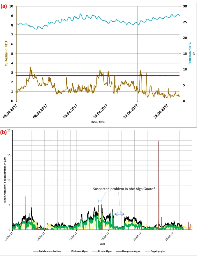
4.2. Feed Water Quality

Temperature, pH, turbidity, feed flow rate, pressure at feed and filtrate sides were constantly monitored. Hourly averages of feed water quality for temperature, pH and turbidity are shown in Figure 18a.

25 Figure 18: Feed water quality for (a) hourly average for temperature, pH and turbidity (b) Total and various algae groups’

concentration.

The feed water quality was relatively good, with constant pH around 8.0, temperature between 22°C to 28°C, and turbidity less than 5 NTU. Table 6 shows a summary of the averages, standard deviation and range of values of the parameters.

Suspected problem in bbe AlgalGuard®

(b)

(a)

26 Table 6: Feed water quality of PU 22.

Parameters Units Average Standard

Deviation Range Reference values [47] Turbidity NTU 1.47 1.99 0.08 - 11.05 2-10

pH - 8.00 0.01 7.94 - 8.02 -

Temperature _{°C 25.5 1.2 22.7 - 28.1 15.0 - 36.3} Total chlorophyll-a _{µg/l 2.0 0.88 1.0 – 4.5 0.82 - 1.49 ± 0.33}

Concentration of chlorophyll-a, diatoms algae, green algae (Chlorophytes), blue-green algae (cyanobacteria) and cryptophyta were measured and recorded by bbe AlgalGuard® every 97 seconds. It is considered an algal bloom event when the total chlorophyll-a concentration is more than 15 µg/l [22]. Referring to Figure 18b, there was no algal bloom during the period of experiment. However, certain trends were observed when the concentration was more than 4µg/L. The total chlorophyll–a concentration of feed water will be plotted alongside the performance chart. There was also some period of time where a problem in bbe AlgalGuard® was suspected to be not working. The data from these periods were removed during feed water correlation analysis.

The parameter settings for filtration, rcBW and CEB during the experiments can be found in

APPENDIX C.

The methods used for analysis were (1) regression for Total Fouling and Hydraulic Irreversible Fouling Indices and (2) change in permeability. Both methods will be discussed in detail in the following section.

4.3. Methods used for determining the efficiency of cleaning

Being able to predict fouling in membranes is crucial, yet, highly complex as it depends on the feed water’s physiochemical properties alongside the type of membrane used and the process parameters (TMP, filtration flux etc.) [48].

It is also challenging as certain feed water parameters such as Total Organic Carbon, Total Suspended Solids etc. are not measured constantly. Constantly sampling of feed water can be expensive and is not real-time monitoring. From the process point of view, it is useful to analyse the available parameters and fouling indices (calculated from the parameter data) which are measured constantly.

27

4.3.1.

Fouling Indices

In general, feed water with high values of turbidity and TSS tends to cause severe fouling. However, the work of Zupancic et. al. [49] showed that turbidity is not directly correlated with fouling and is not sufficient as a sole indicator for fouling prediction.

Natural water sources containing high amount of Total Organic Carbon, Dissolved Organic Carbon and Natural Organic Matter (NOM) also tend to cause fouling. Different measures of NOM include Total Nitrogen, Dissolved Organic Nitrogen, ultraviolet absorbance, NOM molecular weight distribution, and NOM source have been found to have certain impacts on membrane fouling but no single characteristic has been demonstrated to control fouling [50-52].

The drawback of using these parameters is that they cannot be constantly monitored online and in real time easily. Constant sampling to test for these parameters will induce high operational cost. Over the years, simple, short and empirical filtration tests had been developed to obtain fouling indices to predict degree of membrane fouling.

The silt density index (SDI) and modified fouling index (MFI) are widely used in RO applications. Unfortunately, they have been reported to be insensitive to the presence of smaller particles and an unsatisfactory correlation with colloidal fouling has been observed for full-scale membrane installations [53, 54]. The MFI-UF (tested with a polyacrylonitrile 13 kDa UF membrane) was developed to account for the presence of smaller particles but at constant pressure [53, 54].

A group of researchers [52, 55-57] proposed a unified MFI for assessments of low pressure membrane performance at constant flux with the assumption that fouling is caused only by cake layer formation. It is in doubt if bench-scale or full-scale data can be compared with this unified MFI [48].

In the case of inge GmbH, the fouling index of Hydraulic Irreversible Fouling Index (HIFI) were chosen as the analysis tool. Together with Total Fouling Index (TFI) and Chemical Irreversible Fouling Index (CIFI), these indices were developed by A.H. Nguyen and co-workers [48] and were based on a resistance in-series model. The indices indicate the rate of increase in resistance due to fouling, i.e., smaller indices indicate slower rate of increase in resistance. The key feature of this development is that fouling is not attributed to a specific mechanism so the model is valid regardless of whether cake filtration, pore constriction, or a combination of fouling mechanisms occurring. The full derivation is available in APPENDIX D and the final form is summarized in Table 7.

28 Table 7: Summary of fouling indices developed by A.H. Nguyen et. al. [48].

Total Fouling Index (TFI)

Hydraulic Irreversible Fouling Index (HIFI)

Chemical Irreversible Fouling Index (CIFI)

Any single hydraulic backwash

Multiple hydraulic backwash cycles without any chemical cleaning (referred to as one chemical cleaning cycle)

Average values for all data for a series of chemical cleaning cycles

1

Perm′

= 1+ (TFI)S

1

Perm′

= 1+ (HIFI)S

1

Perm′

= 1+ (CIFI)S

Perm’: normalized permeability (or specific flux) [-] Svol: specific volume [m

3

/m2]

29

4.3.2.

Change in permeability

The most classical way for determining the physical cleaning’s efficiency is to look at the permeability of the process. With reference to Figure 20, the permeability of the membrane process will drop over time due to fouling’s additional resistance to permeation. The change in permeability (∆Perm) before and after each rcBWs/CEBs gives a simple and general indicator on the removal of foulants.

Both methods of fouling indices and different in permeability will be used for comparison of the efficiency of Capillary Drain in this work.

4.4. Data Evaluation

The process of the data evaluation is illustrated in Figure 21.

Figure 21: Steps of conducting data analysis.

Continuous logging of data

Import into MS Access® database

Export into MS Excel® file

Generate performance chart

Calculate key performance indicators

30 Physical parameters of PU 22 pilot plant were logged. 44 of them were written into .csv files every 45 seconds during filtration and CEB. Backwash and Capillary Drain were written every second. These daily reports were imported into an MS Access® database, which can be exported to MS Excel® files for generation of performance charts. Flux was evaluated by dividing the recorded feed flow rate by the active membrane area of 80 m2. TMP was evaluated by difference of pressure between the feed and filtrate side, with correction for the hydrostatic pressure using Eq.3. Permeability was evaluated by dividing the flux by TMP and then normalized to 20°C using Equations 5 and 6. Key performance indicators (Total Fouling and Hydraulic Irreversible Fouling Indices) were calculated using built-in regression function RGP in MS Excel®.

These data, together with parameters of feed water and filtrate, were fed into the statistical program Minitab® 2017 to investigate for potential correlations. Further details will be explained separately in Section 6.

31

5. Results and discussion

This section describes the results obtained from the pilot plant for discussion of effect of Capillary Drain.

5.1. Effect of Capillary Drain

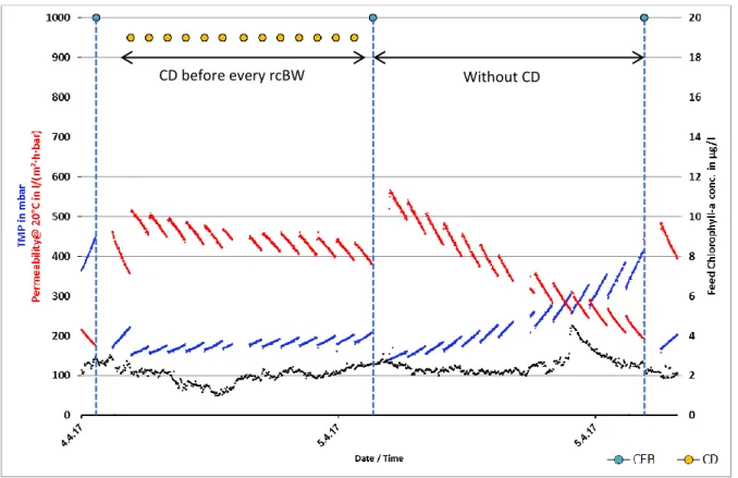
Figure 22 illustrates the membrane process’s performance of Line 2 with and without Capillary Drain. Blue-filled circles and yellow-filled circles represent the introduction of CEB and Capillary Drain, respectively. Unless otherwise stated, Capillary Drain was always conducted after one filtration cycle.

Figure 22: Performance of Line 2 at filtration flux and time of 85 l/(m²·h) and 50 minutes, BW flux and time of 230 l/(m²·h)

and 35 seconds, CEB interval of 14.

Remarks for Figure 22

- CEB interval of 14 means that CEB was conducted after 14 filtration cycles.

- A peak of more than 4 µg/L of chlorophyll-a was observed on 5 April 2017 around 2223 hours lasting around 1.5 hours. Despite of this, performance of Line 2 did not show abrupt changes for TMP and permeability.

The positive effect of Capillary Drain is clearly shown in Figure 22. For the chemical cleaning cycle when Capillary Drain was introduced before every rcBW, the rate of permeability decrease was slower

32 than chemical cleaning cycle without Capillary Drain. To demonstrate this with Hydraulic Irreversible Fouling Index, “Normalized inverse permeability” was plotted against the specific volume in Figure 23 and the slope was determined. Without Capillary Drain, the Hydraulic Irreversible Fouling Index value is 1.3653 m2/m3 as compared to 0.2127 m2/m3 for Capillary Drain conducted before every rcBW. Clearly, Capillary Drain had slowed down the rate of increase in resistance. It is important to note that the regression of Total Fouling and Hydraulic Irreversible Fouling Indices follows the method proposed by A.H. Nguyen et. al. [48] using linear regression. This method for obtaining Total Fouling and Hydraulic Irreversible Fouling Indices are meant for interpretation of results and not trying to fit the best model with the experimental data.

Figure 23: Hydraulic Irreversible Fouling Index plot for chemical cleaning cycle with Capillary Drain before every rcBW

(red) and without Capillary Drain (green).

Remarks for Figure 23

- The “high peaks” in the Hydraulic Irreversible Fouling Index plots were caused in one line when the other was in backwash mode.

- The change in R2 was < 1% and change in Hydraulic Irreversible Fouling Index values were < 3% when these points were removed manually. This was deemed acceptable by inge GmbH and thus, the data points were kept.