Key words – Adaptive control; Predictive control; canal control; water distribution
João M. LEMOS∗, Luís M. RATO∗*, F. MACHADO∗** , Nuno NOGUEIRA∗**, Pedro SALGUEIRO∗***, Rui N. SILVA∗****, Manuel RIJO∗*****
PREDICTIVE ADAPTIVE CONTROL OF WATER LEVEL IN CANAL POOLS
A case study on the use of a predictive adaptive algorithm to control pool level in a pilot water distribuition canal is described. The algorithm is a modification of the basic MUSMAR controller that includes parallel integral action and, in the case of multiple pools, feedforward action to coordinate the gates. Experimental results in the case of a single pool and simulations for multiple pools are presented. The contributions of the paper stem from the explicitation of rules for tuning the adaptive controller in a practical situation and from the coordination of different pools using reduced complexity controllers and feedforward in a multivariable setting.
1. INTRODUCTION
The problem considered in the paper is the control of the pool level in a pilot water distribution canal. This problem has been the subject of a lot of attention, of which [1-5] are representative examples. The main difficulties are unmodelled dynamics (the plant is infinite dimensional), variable transport delays and strong interactions between the different subsystems (pools). While the generatility of existing references depart from a model that is initially identified, serving then as a basis for controller design, the approach followed in this paper relies on adaptive control and hence allows for changes of the canal dynamics due to unpredictable factors that slowly act over time. This approach has also the advantage of not requiring the expensive initial phase of modelling.
In order to control the canal the predictive adaptive MUSMAR algorithm was selected [6]. This algorithm has a number of advantageous features such as a certain degree of insensivity with respect to plant i/o transport delay and unmodelled dynamics [7]. It has been applied to several industrial or large scale plants with distributed parameter dynamics including industrial boilers [8], arc welding [9] and distributed collector solar fields [10].
∗ INESC-ID/IST, R. Alves Redol 9, 1000-029 Lisboa, Portugal, [email protected]. Corresponding author. The work
reported in this paper was performed under project FLOW, POSC/EEA-SRI/61188/2004, supp. by POSC and FEDER, and NiSIS (Nature Inspired Smart Information Systems) network.
**
Departamento de Informática, Universidade de Évora, 7000 Évora, Portugal, [email protected].
∗**
INESC-ID/IST, R. Alves Redol 9, 1000-029 Lisboa, Portugal.
∗***
INESC-ID/IST, R. Alves Redol 9, 1000-029 Lisboa, Portugal.
∗****
Departamento de Informática, Universidade de Évora, 7000 Évora, Portugal, [email protected].
∗*****
Dep. de Eng. Electrot. e de Computadores, Fac. De Ciências e Tecnologia, Univ. Nova de Lisboa, [email protected]
∗******
The present paper includes results for a single pool as well as for multiple pools. Both the objectives of tracking a reference and regulating the level in the presence of disturbances for each pool level are considered. The paper is organised as follows: After this introduction, the plant is described in section 2. Section 3 describes the algorithm and its adaptation to the problem at hand and section 4 presents experimental and simulation results. Conclusions are drawn in section 5. 2. PLANT DESCRIPTION
The plant to be controlled is the experimental canal of Núcleo de Hidráulica e Controlo de Canais of UNiversidade de Évora, located in the south of Portugal. Figs. 1 and 2 show a general view of it. It has been the subject of other studies, e. g. [4].
1. Overall view of the experimental canal.
2. The end of the computer controlled canal with gate 3 (foreground) and gate 4 (background) and the beginning of the returning traditional canal (feft). On the right the wells where two level sensors are installed can be seen.
H0 C1 C2 C3 C4 J1 M1 J2 M2 J3 M3 M4 Di scharge Q1 Q2 Q3 Q4 Reservoir u1 u2 u3 u4
Gate 1 Gate 2 Gate 3
Gate 4 Pool 1
Pool 2
Pool 3
Pool 4
3. Schematic view of the experimental computer controlled canal.
The canal has 141 m long and is divided in 4 pools, separated by gates. A SCADA system allows to perform computer control of the system with a sampling interval of 1 s. From the systems point of view, this is a distributed parameter system with 4 inputs (the gate position commands), 4 outputs (the level of each pool measured just before each gate) and 4 disturbances (water flow outlets in each pool). Fig. 3 shows a schematic view of the canal, with the main variables indicated.
3. THE CONTROL ALGORITHM
Many natural systems rely on multiple individual actions that combine in a probabilistic way to yield the desired result. In a control framework, this inspires a structure where the control decision is based on the probabilistic merging of multiple agents, such as shown in fig. 4. Each agent receives the same plant signals but takes partial decisions assuming different scenarios. A probabilistic combination of these partial actions yields the final control decision.
Probabilistic combination of actions . . . Plant feedbac k information Agent 1 Agent N Final control decision Partial control decisions under different scenarios
3. Control decision based on the probabilistic merging of multiple agents.
In an ideal situation (perfect modelling, complete state information, no disturbances, no nonlinearities), only one agent (one controller, based on a single plant model) would be enough to achieve a high performance controller. In the presence of non-ideal factors, however, a controller based on just one agent is prone to yield incorrect control actions. If, instead, the controller is based on multiple agents (simpler controllers based on different plant models), the diversity thereby introduced leads to increased performance and robustness properties.
s( t)
T-s teps ahead predictor
2- steps ahead predictor
1- step ahead predictor
Constant feedback acting on the plant
t t+1 t+2 t+T
. . .
. . . Pres ent time
u(t)=?
4. Diversity based plant description using multiple predictors sharing a common regressor build from plant data, assuming a constant feedback from t+1 up to t+T.
In order to achieve a practical control algorithm, the plant I is described (fig. 4) by multiple predictive models, sharing a common regressor. Assuming a constant feedback to act on the plant, the predictive models are described by
) ( ) ( ' ) ( ) (t i u t s t v t y + =θi +ψi + i i=1 K, ,T
where u is the manipulated variable, y is the deviation of the output of the system to control with respect to the set-point, v and w are residues orthogonal to the data in a least squares sense and
i i i i ψ µ φ
θ , , , are parameters to be extracted from plant data using Least Squares. The pseudo-state vector s(t) is made from samples of past plant data and defines the controller structure. An example is
[
( ) ( 1) ( 1) ( ) ( ) ( 1)]
' : ) (t = y t y t−n+ u t− u t−m w t w t− p+ s L L Lwhere wis an auxiliary signal (system’s internal variable or accessible disturbance). Each of the individual agents is designed such as to minimize the single-step horizon i steps ahead cost functional given by
[
t]
i t E y t i u t i I
J ( )= 2( + )+ρ 2( + −1)| i =1 K, ,T
where E |
[ ]
o It is the mean conditioned on the available observations up to time t , I . ts( t) F1 F T
+
u( t) u1(t) uT(t)Control ac tion merger π 1 π T . . . . . .
5. Realization of the MUSMAR control [6] law by merging T self-tuners, each matched to a single-step horizon i-steps ahead cost functional. Compare with fig. 2.
) ( ) ( ) ( ) 1 (t i 1u t 1s t w 1 t u + − =µi− +φi− + i−
The control action generated by the partial controller (agent) i is given by a feedback from the pseudo-state s(t) ) ( ' ) (t F s t ui = i i=1 K, ,T with
(
1 1)
2 1 2 1 − − − + + = i i i i i i i F θ ψ ρµ φ µ ρ θand the probabilistic weights for merging these actions are given by [2] (see fig. 4 for a block diagram that parallels fig. 2):
(
)
∑
= − − + + = T j j j i i i 1 2 1 2 2 1 2 ρµ θ µ ρ θ πActually, this multiple actions merge to yield the control action simply defined by
) ( ' ) (t F s t u = with
(
)
∑
∑
= − = + + − = T i i i T i i i i i F 1 2 1 2 1 µ ρ θ φ µ ρ ψ θThis controller has a number of interesting features that are a consequence of the diversity features that it embodies. In particular, the update of the gain vector F is made suich as to minimize the steady state quadratic cost defined by
[
( ) ( )]
limE y2 t u2 t J t +ρ = ∞ → ∞ y( t) y( t-T+1|t- T) ^ Prediction er ror 1 Parameter update y( t) y( t-T+1|t- T) ^ Prediction er ror 1 Parameter update Delay T s( t) Plant data Covariance matrix ( P) update Kalman gain computation P(t) s( t-T) Kalman gainx
x
+
+
-Θ
Θ
1 T . . . Predictor 1 parameter es timates Predictor T parameter es timates6. Multiple predictors parameter update from plant data, using a common Kalman gain and redundant estimates.
Indeed, the update of F in two consecutive time steps is given by )) 1 ( ( 1 ) 1 ( ) (t =F t− − R−1∇ J∞ F t− F s T α
where 21 1 2 − = + =
∑
j T j j ρµ θα , R is an approximation of the Hessian matrix of s J and ∞ ∇TJ∞(F(t−1)) is an approximation of the gradient of the steady state cost with respect to the cost. Hence, the controller acts as an approximation to a Newton type minimization algorithm that seeks the minimum of the steady state quadratic cost. Furthermore, this approximation becomes better when the number of predictive models (the diversity) increases.
Separate MUSMAR controllers are employed for each pool, but with feedforward signals designed in such a way has to coordinate them. This is achieved by using as accessible disturbance in each controller the sum of the tracking error of the precedent pools. Furthermore, a low gain integrator is used in pareallel to eliminate stationary tracking errors (fig. 7).
Ref
MUSMAR Canal Pool
Ki /s
u m
+
-+
+
7. Block diagram of the controller:MUSMAR with the parallel integrator.
4. RESULTS
Figs. 8 and 9 show experimental results for a single pool. The configuration used was T =10
2800 2850 2900 2950 3000 3050 3100 3150 3200 3250 400 450 500 m a n d r e f [m m ] 28000 2850 2900 2950 3000 3050 3100 3150 3200 3250 100 200 300 400 time [samples] u [ m m ] 2800 2850 2900 2950 3000 3050 3100 3150 3200 3250 -0.2 -0.1 0 kin t 28000 2850 2900 2950 3000 3050 3100 3150 3200 3250 100 200 300 uin t [ m m ] 2800 2850 2900 2950 3000 3050 3100 3150 3200 3250 0 100 200 Time [samples] uM U S M A R [ m m ]
8. Tracking a reference level. Left: model and reference (top) and manipulated variable (bottom). Right: Contribution of the integral effect (middle) and of MUSMAR (bottom) to the manipulated variable. Experimental results with one
pool.
3
=
n , m=2, ρ =0.01 and KI =−0.02. Fig. 8 (right) shows how MUSMARE and the parallel integrator conjugate their control actions. MUSMAR acts essentially during the transients, providing a fast response, while the integrator adjusts the gate position during steady state to achieve zero tracking error.
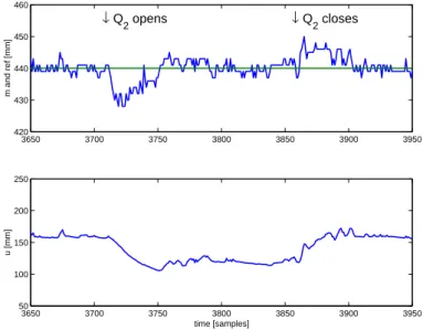
Fig. 9 shows experimental results on disturbance rejection. The disturbances are induced by opening the exterior outlet to simulate the use of water for irrigation. When the outlet Q2opens, the gate closes to compensate the loss in water flow.
3650 3700 3750 3800 3850 3900 3950 420 430 440 450 460 m and ref [mm] ↓ Q 2 opens ↓ Q2 closes 3650 3700 3750 3800 3850 3900 3950 50 100 150 200 250 time [samples] u [mm]
9. Rejecting disturbances due to the opening of the external outlet: Measured level and constant reference (above) and manipulated variable (below).
Figs 10 and 11 show simulation results when the four pools of the canal are controlled each with a MUSMAR controller having an integrator in parallel. The simulation was performed using a SIMULINK model based on the numeric integration of the Saint-Venant equations that has been calibrated with plant data.
In a practical situation, a canal is usually operated with a constant reference. In this case, for the sake of testing the dynamic response of the controlled canal, the reference of pools 1 and 3 is made to vary in alternation, according to squared signals. This induces disturbances from the one pool into the others, resulting in frequent level changes.
In the case of fig. 11 there is a feedforward included in the pseudo-state made from the sum of the tracking errfors of the previous pools, while for fig. 10 this feedforward action is not used. The rationale for this consists in the fact that the controller of a pool will act to compensate the existing tracking error and this results in the retention of release of a certain quantity of water that will disturbe the down-stream pools forcing their controllers, in turn, to react. The feedforward action allows a corrective action that anticipates the effect of the water expected to arrive due to the action of the upstream controllers.
As can be seen by comparying both figures, the feedforward action results in oscillations of small amplitude.
3.6 3.65 3.7 3.75 3.8 3.85 3.9 3.95 4 4.05 x 10⁴ 0 0.2 0.4 0.6 0.8 Time (s) Level (m) M1 Reference Measure 3.6 3.65 3.7 3.75 3.8 3.85 3.9 3.95 4 4.05 x 10⁴ 0 0.2 0.4 0.6 0.8 Time (s) Level (m) M2 Reference Measure 3.6 3.65 3.7 3.75 3.8 3.85 3.9 3.95 4 4.05 x 10⁴ 0 0.2 0.4 0.6 0.8 Time (s) Level (m) M3 Reference Measure 3.6 3.65 3.7 3.75 3.8 3.85 3.9 3.95 4 4.05 x 10⁴ 0 0.2 0.4 0.6 0.8 Time (s) Level (m) M4 Reference Measure
5000 5500 6000 6500 7000 7500 8000 8500 9000 9500 0 0.2 0.4 0.6 0.8 Time (s) Level (m) M1 Reference Measure 5000 5500 6000 6500 7000 7500 8000 8500 9000 9500 0 0.2 0.4 0.6 0.8 Time (s) Level (m) M2 Reference Measure 3.6 3.65 3.7 3.75 3.8 3.85 3.9 3.95 4 4.05 x 10⁴ 0 0.2 0.4 0.6 0.8 Time (s) Level (m) M3 Reference Measure 5000 5500 6000 6500 7000 7500 8000 8500 9000 9500 0 0.2 0.4 0.6 0.8 Time (s) Level (m) M4 Reference Measure
11. Tracking a reference level. Level and reference of the four pools when all pools are controlled with MUSMAR with feedforward.
5. CONCLUSIONS
The paper shows how to configure a predictive adaptive controller in a practical situation. Prediction over extended horizon is needed for tackling the difficulties associated with the variable delays associated to the transport phenomena (water displacement). The redundancy in the identification of the predictive models helps tackling unmodeled dynamics inherent to an infinite order (distributed) plant. Furthermore, this is a multivariable plant with strong interaction between the different parts. Although MUSMAR could be configured as a multivariable controller, this would yield severe identifyability problems. The results show that the feedforward scheme proposed allows to achieve a good perfcormance due to a balance between pool coordination and reducing the identifyability problems.
REFERENCES
[1] S. Sawadogo, P. Malaterre and P. Kosuth. Multivariable optimal control for on-demand operation of irrigation canals, Int. J. System Science 26(1):161-178 (1995).
[2] G. Corriga, S. Sanna and G. Usai. Sub-optimal constant-volume control for open channel networks. Applied Math. Modelling, 7:262-267 (1983).
[3] J.-M. Coron, B. d’Andréa-Novel and G. Bastin. A Lyapunov approach to control irrigation canals modelled by Saint-Venant’s equations, European Contropl Conf. 1999, Karlsruhe, Germany.
[4] X. Litrico, V. Fromion, J. P. Baume and M. Rijo. Modelling and PI control of an irrigation canal. European Control Conf., Cambridge, U. K. (2003).
[5] X. Litrico and V. Fromion. H∞ control of an irrigation canal pool with a mixed control politics, IEEE Trans. Control Syst. Techn. 14(1):99-111 (1995).
[6] Greco, C., G. Menga, E. Mosca and G. Zappa (1984). Performance improvements of self-tuning controllers by multistep horizons: The MUSMAR approach. Automatica, 20(5): 681-699.
[7] Mosca, E., G. Zappa and J. M. Lemos (1989). Robustness of Multipredictor Adaptive Regulators: MUSMAR. Automatica, 25(4): 521-529.
[8] Silva, R. N., Shirley, P. O., J. M. Lemos and A. C. Gonçalves. Adaptive regulation of super-heated steam temperature: A case study in an industrial boiler. Control Engineering Practice, 8 (2000):1405-1415.
[9] Santos, T. O., R. Caetano, J. M. Lemos and F. J. Coito. Multipredictive adaptive control of arc welding trailing centerline temperature. IEEE Trans. Control Syst. Technol. 8 (2000): 159-169.
[10] Coito, F.; J. M. Lemos, R. N. Silva and E. Mosca (1997). Adaptive control of a solar energy plant: Exploiting accessible disturbances. Int. J. Adaptive Control and Signal Proc., 11:327-342.