A Bayesian approach for constructing genetic maps when markers are miscoded

DOI: 10.1051/gse:2002012

Original article

A Bayesian approach for constructing

genetic maps when markers are miscoded

Guilherme J.M. R

, Brian S. Y

,

Daniel G

a

Department of Biostatistics, UNESP, Botucatu, SP, Brazil

b

Departments of Statistics and of Horticulture, University of Winconsin, Madison, WI, USA

c

Departments of Animal Science and of Biostatistics & Medical Informatics, University of Wisconsin, Madison, WI, USA

(Received 10 September 2001; accepted 8 February 2002)

Abstract – The advent of molecular markers has created opportunities for a better understanding of quantitative inheritance and for developing novel strategies for genetic improvement of agricultural species, using information on quantitative trait loci (QTL). A QTL analysis relies on accurate genetic marker maps. At present, most statistical methods used for map construction ignore the fact that molecular data may be read with error. Often, however, there is ambiguity about some marker genotypes. A Bayesian MCMC approach for inferences about a genetic marker map when random miscoding of genotypes occurs is presented, and simulated and real data sets are analyzed. The results suggest that unless there is strong reason to believe that genotypes are ascertained without error, the proposed approach provides more reliable inference on the genetic map.

genetic map construction / miscoded genotypes / Bayesian inference

1. INTRODUCTION

The advent of molecular markers has created opportunities for a better understanding of quantitative inheritance and for developing novel strategies for genetic improvement in agriculture. For example, the location and the effects of quantitative trait loci (QTL) can be inferred by combining information from marker genotypes and phenotypic scores of individuals in a population in

linkage disequilibrium, such as in experiments with line crosses, e.g., using

backcross or F2 progenies. A QTL analysis relies on the availability of

accurate estimates of the genetic marker map, which includes information

∗_{Correspondence and reprints}

E-mail: [email protected]

on the order and on genetic distances between marker loci order. Genetic maps are inferred from recombination events between markers, which are genotyped for each individual. Several statistical methods have been

sug-gested for map construction. Lathrop et al. [14], Ott [17] and Smith and

Stephens [21] discussed maximum likelihood procedures for marker map

inferences, and Georgeet al.[9] presented a Bayesian approach for ordering

gene markers. Jones [10] reviewed a variety of statistical methods for gene

mapping. At present, most statistical methods used for map construction

ignore the possibility that molecular (marker) data may be read with error. Often, however, there is ambiguity about genotypes and, if ignored, this can adversely affect inferences [3, 15]. The problem of miscoded genotypes has received the attention of some investigators. Most of their research, however, has focused on error detection and data cleaning [4, 11, 15]. The objective of our work is to discuss possible biases in marker map estimates when miscoding of genotypes is ignored and to suggest a robust approach for more realistic inferences about marker positions and their distances. The approach simultan-eously estimates the genotyping error rate and corrects for possible miscoded genotypes, while making inferences on the order and distances between genetic markers.

The plan of the paper is as follows. In Section 2, the problem of miscoding genotypes is discussed, as well as the systematic bias that this imposes on genetic map estimation. In Section 3, a Bayesian approach for inferences about a genetic map, when miscoding is ignored, is reviewed. In Section 4, the methodology is extended to handle situations with miscoded genotypes, when these occur at random. Simulated and real data are analyzed in Sections 5 and 6, respectively, and the results are discussed. Concluding remarks are presented in Section 7.

2. THE PROBLEM CAUSED BY MISCODED GENOTYPES

First consider the estimation of the genetic distance between two marker loci

having a recombination rateθ. In simple situations,e.g., with double haploid

or backcross designs, each individual has one of two possible genotypes (say 0 or 1) at each marker locus. Inferences about genetic distance between loci are based on recombination events, which are observed by genotyping individuals. If marker genotypes could be read without error, the probability of observing

a recombination event in a randomly drawn individual would beθ. However,

it will be supposed that there is ambiguity in the assignment of genotypes to

individuals. For example, a genotype 0 may be coded as 1 (or vice-versa),

with probabilityπ. Here, given the genotype for a specific marker and the

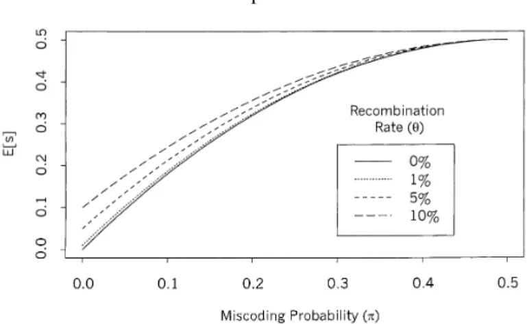
Figure 1.Expected recombination events observed on different values of miscoding probabilities (π_{), for some selected values of recombination rates (}θ_).

written as:

p[mij|gij,π] =π|mij−gij|(1−π)

1−|mij−gij|_,

wheremijandgijare the observed and true genotypes (mij,gij =0,1),

respect-ively, for locusj(j=1,2) of individuali(i=1,2, . . . ,n).

If a “recombination event” between the loci is observed, this may be due to either a true genetic recombination between them, or to an artifact caused by miscoding. Hereinafter, a “recombination” observed by genotyping the mark-ers will be denoted as the “apparent recombination”, to distinguish between observed and “true” recombination events.

The probability of observing an apparent recombination between markers 1

and 2 for individualican be written as:

Pr(si =1)=Pr[ri=1](Pr[no miscod.] +Pr[double miscod.])

+Pr[ri=0]Pr[one miscod.]

=θπ2+(1−π)2+2(1−θ)π(1−π)

=θ+2π(1−π)(1−2θ), (1)

wheresi = |mi1−mi2|andri = |gi1−gi2|stand for apparent and real

recom-bination events, respectively; and Pr[ri=k] =θk(1−θ)1−k, withk=0,1.

It is easy to realize, therefore, that recombination rates estimated from recombinations observed by genotyping the marker loci, ignoring the possib-ility of miscoding, would be biased upwards whenever the markers are linked

(θ < 0.5) andπ > 0. Figure 1 shows the expected apparent recombination

rates as function ofπ, for some selected recombination rate values. It seems

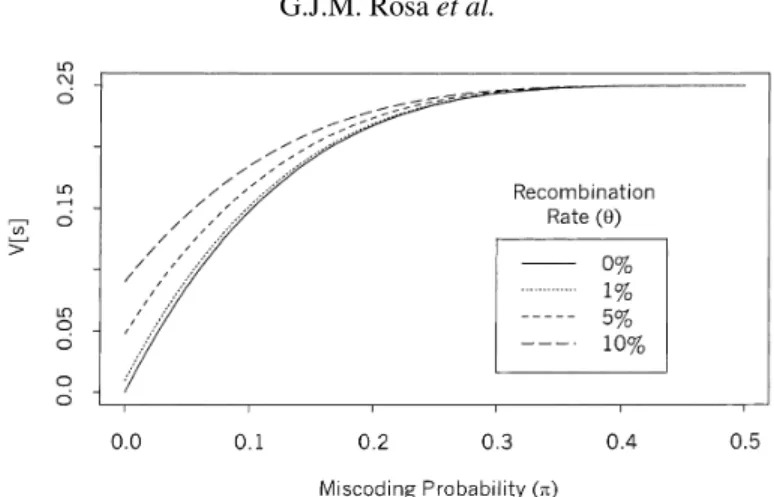
Figure 2. Variance of recombination events observed on different values of miscoding probabilities (π_{), for some selected values of recombination rates (}θ_).

The variance of the apparent recombination event is equal to:

Var[si] =Pr[si=1](1−Pr[si=1])

= [θ+2π(1−π)(1−2θ)][1−θ−2π(1−π)(1−2θ)]

=θ(1−θ)+2π(1−3π+4π2−2π3)(1−2θ)2. (2)

Thus, the variance of apparent recombination events is larger than the variance

of the real recombination events whenever the markers are linked(θ < 0.5)

andπ>0. Figure 2 shows the variance of the apparent recombination events

as a function ofπ, for some different values of recombination rates.

In view of the possibility of miscoding for each marker genotype (i.e.

ambi-guity about their genotypes), standard methods commonly used for genetic map inferences overestimate the recombination rate between loci (or, in other words, underestimate genetic linkage), and underestimate its precision [15]. For example, the maximum likelihood estimator of the recombination rate between the loci (if the possibility of miscoding is ignored) is:

ˆ

θ= 1

n

n

X

i=1

|mi1−mi2|,

with expectation and variance given by (1) and (2), respectively.

In more general situations, we have more than just two marker loci, and

the goal is to construct the genetic map,i.e., to order these marker loci and to

estimate the genetic distances between them. Again, all inferences are based on recombination events observed (apparent recombinations) between the marker loci. The problem of ignoring miscoding may lead to even worse difficulties,

3. BAYESIAN APPROACH FOR GENETIC MAP CONSTRUCTION

First, we will review a Bayesian approach for map construction when

mis-coding is not taken into account [9]. Consider the genotype ofmmarkers for

the individualiasgi=(gi1,gi2, . . . ,gim). In a backcross design, for example,

gij =0 if the individualiis homozygous for the locusj, and 1 otherwise. The

sampling model ofgi, assuming the Haldane map function, is given by:

p(gi|λ,θ)∝ m−1

Y

j=1

θ|gij−gi,j+1|

j (1−θj)

1−|gij−gi,j+1|, (3)

whereλis the order of the genetic marker loci andθjis the recombination rate

between the locijandj+1. Considering a sample ofnindependent individuals,

the likelihood ofλandθis given by:

L(λ,θ|G)=p(G|λ,θ)=

n

Y

i=1

p(gi|λ,θ)

∝

n

Y

i=1

m−1

Y

j=1

θ|gij−gi,j+1|

j (1−θj)

1−|gij−gi,j+1|, (4)

whereGis the(n×m)matrix of marker genotypes, with each row representing

one individual, and each column related to one marker locus.

In a Bayesian context, rather than maximizing the likelihood, it is modified by a prior and integrated to produce inference summaries for the unknown components in the model. The prior can be chosen based on earlier studies or information from the literature. Here, we use a prior expressed as:

p(λ,θ|τ,α,β)=p(θ|λ,α,β)p(λ|τ), (5)

where p(λ|τ) is a probability distribution over the m!/2 different orders

for the m markers, τ is a set of prior probabilities of each order, and

p(θ|λ,α,β) = Qm−1

j=1 p(θj|λ,αj,βj), where θj|λ,αj,βj~Beta(αj,βj) is the

recombination rate between genetic markersj andj+1. A special case of

these prior distributions would be uniform across different gene orders, and

Uniform(0,0.5)distributions for eachθj.

The Bayes theorem combines the information from the data and the prior knowledge to produce a posterior distribution over all unknown quantities. In

this case, the posterior density ofλandθis given by:

p(λ,θ|G,τ,α,β)∝p(G|λ,θ)p(θ|λ,α,β)p(λ|τ). (6)

3.1. Fully conditional posterior distributions

The Gibbs sampler draws samples iteratively from conditional posterior distributions deriving from (6). The fully conditional posterior distribution of

each recombination rateθjis:

p(θj|λ,G,τ,α,β)∝θ

αj−1

j (1−θj)βj−

1

n

Y

i=1

θ|gij−gi,j+1|

j (1−θj)

1−|gij−gi,j+1|

∝θqj+αj−1

j (1−θj)n−qj+βj−

1

, (7)

whereqj=

Pn

i=1|gi,j−gi,j+1|is the number of recombination events between

the locijandj+1. This is the kernel of a Beta distribution with parameters

(qj+αj)and(n−qj+βj).

The updating for the gene orderλinvolves moves between a set of models,

because for distinct ordering, the recombination rates have different meanings.

Georgeet al.[9] discuss a reversible jump algorithm, for which recombination

rates are converted into map distances, and reverted to new recombination rates after shifting a randomly selected marker around a pivot marker.

Here, another Metropolis-Hastings [12] scheme is presented for the MCMC

updating ofλandθ, simultaneously. A new gene ordering is proposed according

to a candidate generator densityq(.), and new recombination rates are simulated

for this new order, using (7). The Markov chain moves from the current state

T =(λ,θ)toT∗_=(λ∗_,θ∗_{)with probability:}

π(T∗,T)=min

1,p(λ

∗_,θ∗_|G,τ,α,β)

p(λ,θ|G,τ,α,β)

q(λ,λ∗₎ q(λ∗_,λ)

, (8)

where p(λ,θ|G,τ,α,β) is the joint conditional posterior distribution of the

gene orderingλand recombination ratesθ, given by:

p(λ,θ|G,τ,α,β)∝p(λ|τ)

m−1

Y

j=1

θq_jj+αj−1(1−θj)n−qj+βj−

1 .

Under these circumstances, the choice of q(.)is extremely important for an

efficient implementation of the MCMC, especially in situations with a large

number of marker loci. A bad choice ofq(.)would generate a large number

3.2. Missing data

In practice, some marker genotypes are missing. The missing data can be handled by the MCMC approach, with an additional step for updating each missing genotype based on this fully conditional density. For instance, suppose

gij is missing, the genotype for thej-th marker of the individuali. Its fully

conditional distribution is Bernoulli with probability pij = Pr(gij = 1|G−ij)

given by:

pij =

p(gij =1|θ,G−ij,τ,α,β)

X

k

p(gij =k|θ,G−ij,τ,α,β)

,

where G−ij refers to all elements in G but gij, and k = 0,1. Under the

Haldane independence assumption, p(gij = k|θ,G−ij,τ,α,β) depends just

on the recombination rates between the locus j and its flanking neighbors,

as well as on the genotypes of these neighbor loci, so it can be written as

p(gij =k|θj−1,θj,gi,j−1,gi,j+1).

4. THE PROBABILITY OF MISCODING GENOTYPES

At present, the methods commonly used for map construction ignore the possibility that molecular (marker) data may be read with error, or the error rate has a fixed and known value, as in Lincoln and Lander [15]. Often, however, there is ambiguity about the genotypes. To address these situations,

we introduced a new parameter into the model, the probabilityπof miscoding

a genotype. Now we consider that the matrix G of genotypes is unknown,

and that we observe a matrixMof genotypes, possibly with some miscoding.

The probability of observing a genotypemij, i.e.the genotype of locusj for

individuali, given that the actual genotype isgij, may be expressed as:

Pr(mij=k1|gij=k2)=π|k1−k2|(1−π)

1−|k₁−k₂|_,

wherek1andk2assume values equal to 0 or 1.

Assuming independence between miscodings in different loci and individu-als, and considering that the miscoding rate is constant over the genome, the

probability of observing a matrixMof genotypes, given the matrixGof actual

genotypes, can be expressed as:

p(M|G)=πt(1−π)nm−t, (9)

where n is the number of individuals, m is the number of marker loci, and

t = Pn i=1

Pm

j=1|mij−gij| is the number of miscoding genotypes in the data

an auxiliary and non-observed matrix. The joint posterior distribution of all unknowns in the model is written now as the product of (9) by (4), (5) and the

prior distribution ofπ, which gives:

p(G,λ,θ,π|M,τ,α,β,a,b)

∝πt(1−π)nm−t

n

Y

i=1

m−1

Y

j=1

θ|gij−gi,j+1|

j (1−θj)

1−|gij−gi,j+1|

×p(θ|λ,α,β)p(λ|τ)p(π|a,b). (10)

Assuming a uniform prior probability distribution forλ;Beta(αj,βj)as prior

for eachθj; andBeta(a,b)as the prior distribution forπ, the expression (10)

becomes:

p(G,λ,θ,π|M,τ,α,β,a,b)

∝πa+t−1(1−π)b+nm−t−1

m−1

Y

j=1

θα_jj+qj−1(1−θj)βj+n−qj−

1

whereqj =

Pn

i=1|gij−gi,j+1|, as already defined, is the number of

recombin-ation events between the locijand j+1. Note that the dependence of this

distribution onλis rendered implicit by the definition ofθjas the recombination

rate between the ordered locijandj+1.

4.1. Fully conditional posterior distributions

The fully conditional posterior distributions ofλ and of each θj have the

same forms as discussed before. In the case ofG, its conditional distribution is:

p(G|M,λ,θ,π,τ,α,β,a,b)

∝πa+t−1(1−π)b+nm−t−1

m−1

Y

j=1

θαj+qj−1

j (1−θj)βj+n−qj−

1 .

Given the independence between the recombination events in different intervals

(by the Haldane map function), each element inGcan be updated

independ-ently. Ifj=1,i.e. gij refers to genotypes at one end of the linkage group, its

fully conditional posterior distribution can be written as:

p(gi1|G−i1,M,λ,θ,π,τ,α,β,a,b)

∝π|gi1−mi1|_(1−π)1−|gi1−mi1|_θ|gi1−gi2|

1 (1−θ1)

1−|g_i1−g_i2|_,

For genotypes at interior markers in the linkage group, the fully conditional posterior distribution becomes:

p(gij|G−ij,M,λ,θ,π,τ,α,β,a,b)∝π|gij−mij|(1−π)

1−|gij−mij|

×θ|gij−gi,j−1|

j−1 (1−θj−1)

1−|gij−gi,j−1|θ

|gij−gi,j+1|

j (1−θj)

1−|gij−gi,j+1|,

for j = 2,3, . . . ,m−1. The conditional distribution of the probability of

miscodingπis given by:

p(π|M,G,λ,θ,τ,α,β,a,b)∝πa+t−1(1−π)b+nm−t−1,

which is the kernel of a Beta distribution with parameters(a+t)and(b+nm−t).

5. SIMULATION STUDY

5.1. Example 1

Three data sets were simulated to examine the ability of the model discussed in Section 4 to correctly estimate genetic distances and the probability of miscoding. Each simulation considered 300 individuals with genotypes for 5

loci, denoted asABCDE. The recombination rates between consecutive loci

were assumed to beθAB=0.09,θBC =0.11,θCD=0.05 andθDE=0.14. The

data sets were generated consideringπ=0,0.02 and 0.04, and 3% of missing

data for each.

These data sets were analyzed using models with and without the miscoding

parameter (π). An equal probability distribution was adopted as prior for the

different loci orders. For each recombination rate, aUniform(0,0.5)process

was considered as prior distribution. Computations were performed using the IML procedure of SAS [19]. Graphical inspection and the Raftery and Lewis diagnostic [18] for the Gibbs output using CODA [1] were used for assessing convergence to the equilibrium distribution, the joint posterior. A burn-in period of 1 000 iterations was adopted, followed by 60 000 iterations with thinning intervals of 20, based on a lag-correlation study. Hence, 3 000 samples were retained for the post-Gibbs analysis.

For all data sets, the gene order was estimated perfectly by both models, with

100% of the MCMC iterations sampling the orderABCDE. It seems that, up to

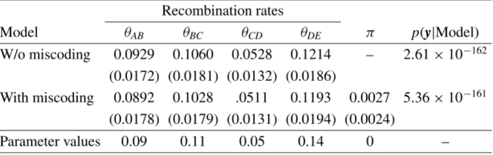
Table I.True parameter values and posterior means and standard deviations (in parenthesis) of the recombination rates considering the data set without miscoding genotypes and the two models, with and without the miscoding parameter.

Recombination rates

Model θAB θBC θCD θDE π p(y|Model)

W/o miscoding 0.0929 0.1060 0.0528 0.1214 – 2.61×10−162 (0.0172) (0.0181) (0.0132) (0.0186)

With miscoding 0.0892 0.1028 .0511 0.1193 0.0027 5.36×10−161 (0.0178) (0.0179) (0.0131) (0.0194) (0.0024)

Parameter values 0.09 0.11 0.05 0.14 0 –

Table I shows the posterior mean and standard deviation for each recombin-ation rate, for the data set without miscoding. The estimates obtained by each model do not present any relevant difference, so it seems that the introduction

of the extra parameter (π) into the model, in situations where there is no

miscoding, does not affect the estimated genetic map. In this example, the

estimate for π was very close to zero, denoting the ability of the model to

recognize situations without miscoding. However, becauseπ=0 relies on the

boundary of the parameter space ofπ, to test for the absence of miscoding for

a particular data set, another approach should be employed, such as comparing

both models (with and without miscoding) using some criteria,e.g., the Bayes

factor or the likelihood ratio test.

The Bayes factors may be computed by taking ratios between estimates of the marginal densities of the data (after integrating out all parameters). If

models are taken as equally probable,a priori, then the Bayes factor gives the

ratio between the posterior probabilities of the corresponding models. Here, the marginal densities were estimated by calculating harmonic means of likelihoods evaluated at the posterior draws of the Gibbs output [16], and these are presented in Table I. The Bayes factor (in favor of the model without the miscoding parameter) of 20.5 does not denote important differences between both models for modeling this data set.

The results obtained by both models for the data set with 2% miscoding

(π = 0.02) are presented in Table II. As expected, the model that ignores

the miscoding problem had estimates biased upwards. When the probability of miscoding was introduced into the model, there was improvement on the estimates. In addition, the probability of miscoding was adequately estimated. For the robust model, all the parameter values were inside a credible set of 0.95

of probability. The Bayes factor of 2.01×106

Table II. True parameter values and posterior means and standard deviations (in parenthesis) of the recombination rates considering the data set with 2% of miscoding genotypes and the two models, with and without the miscoding parameter.

Recombination rates

Model θAB θBC θCD θDE π p(y|Model)

W/o miscoding 0.0982 0.1361 0.0934 0.1950 – 4.70×10−200 (0.0178) (0.0195) (0.0172) (0.0226)

With miscoding 0.0739 0.1096 0.0561 0.1624 0.0223 9.45×10−194 (0.0192) (0.0200) (0.0175) (0.0251) (0.0067)

Parameter values 0.09 0.11 0.05 0.14 0.02 –

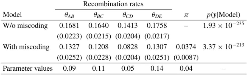
Table III. True parameter values and posterior means and standard deviations (in

parenthesis) of the recombination rates considering the data set with 4% of miscoding genotypes and the two models, with and without the miscoding parameter.

Recombination rates

Model θ_AB θ_BC θ_CD θ_DE π _p(y|Model)

W/o miscoding 0.1681 0.1640 0.1413 0.1758 – 1.93×10−235 (0.0223) (0.0215) (0.0204) (0.0217)

With miscoding 0.1327 0.1208 0.0828 0.1307 0.0374 3.37×10−213 (0.0252) (0.0228) (0.0204) (0.0251) (0.0087)

Parameter values 0.09 0.11 0.05 0.14 0.04 –

Similar results were found for the data set with 4% miscoding (Tab. III).

The Bayes factor, in this case, was of 1.75×1022

in favor of the model with the miscoding parameter.

5.2. Example 2

Thirty data sets were simulated, where half had no miscoding and half had 5% miscoding. Here, our main interest was to examine the performance of the models (with and without miscoding) to correctly estimate the gene order with relatively small data sets, both under situations without miscoding and with high levels of miscoding genotypes. Each data set had 100 individuals with genotypes for five markers; no missing data were considered in this study. The

recombination rates between consecutive loci were: θAB =0.05, θBC =0.18,

θCD=0.02 andθDE =0.07. Prior distributions and computations were similar

to those described for the previous simulation study.

For the 15 data sets without miscoding, both models (with and without

The Bayes factor was favorable to the model without miscoding for 8 of the data sets (and favorable to the model with the miscoding parameter for the remaining data sets), but with no expressive or relevant values (ranging from 1.2 to 57.9). For the datasets with 5% miscoding, the Bayes factor was always favorable to the model considering miscoding genotypes, with values that ranged from

2.42×102

to 8.31×1010

.

The model ignoring the miscoding gave the highest posterior probability for

a gene ordering other thanABCDE in 8 of the 15 data sets. In the case of

the model with the miscoding parameter, just four data sets had the highest posterior probability for a wrong order. If credibility sets with minimum probability of 0.90 are considered, three of the data sets had the correct gene ordering outside of the set. For the model with the miscoding parameter, just one data set presented a probability set that did not contain the correct order.

The results suggest that the model ignoring the miscoding overstates the precision in relation to the gene ordering, sometimes concentrating posterior probability on the wrong (set of) order(s).

6. ANALYSIS OF EXPERIMENTAL DATA

The data set refers to the RFLP study withBrassica napususing F1-derived

double haploid lines. Materials and methods related to the DNA extraction and a preliminary linkage map construction (using maximum likelihood approach)

are presented by Ferreiraet al.[6]. These data, combined with phenotypic

information (flowering time under one of the three vernalization treatments

considered in that study), were also analyzed by Ferreira et al. [5] and by

Satagopanet al.[20] for the study on quantitative trait loci.

Here, we focus on the estimation of the probability of miscoding, and also on robust construction of the linkage map for a set of marker loci. To illustrate the methods, we consider the data for 105 progeny and 10 maker loci related to the linkage group 9, for which 9% of the genotypes were missing. For simplicity,

the marker loci are denoted here by letters (fromAthroughJ), according to the

order that was estimated by Ferreiraet al.[5].

Prior distributions and computations were similar to those describe in Sec-tion 5, for the simulaSec-tion studies. In this case, a longer burn-in period of 2 000 iterations was adopted, followed by 100 000 iterations with thinning intervals of 20. Hence, 5 000 samples were used for the post-Gibbs analysis.

The miscoding rate for this data set was estimated at a level of approximately

1.5%, with a 95% probability set [0.0055; 0.0266]. The model with the

miscoding parameter was much more plausible than the one without it, with the

Bayes Factor of 4.91×106

Table IV.Posterior probabilities of different ordering of the markers in theBrassica

data by using the two models, with and without miscoding.

Models

Order W/o miscoding With miscoding

ABCDEFGHIJ 0.7516 0.6824

BACDEFGHIJ 0.1818 0.1658

ABDCEFGHIJ 0.0412 0.0632

ABCEDFGHIJ 0.0128 0.0404

BACEDFGHIJ 0.0036 0.0094

Others(1) 0.0090 0.0388

(1)_{Loci orders with posterior probabilities smaller than 0.0050.}

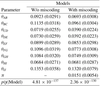
Table V. Posterior means and standard deviations (in parenthesis) of the recombination rates and probability of miscoding in theBrassicadata by using the two models, with and without the miscoding parameter.

Models

Parameter W/o miscoding With miscoding θ_{AB 0.0923 (0.0291) 0.0693 (0.0308)}

θBC 0.1135 (0.0318) 0.0961 (0.0304)

θCD 0.0719 (0.0255) 0.0390 (0.0224)

θDE 0.0730 (0.0259) 0.0392 (0.0223)

θEF 0.0899 (0.0289) 0.0853 (0.0298)

θFG 0.1096 (0.0319) 0.0773 (0.0308)

θGH 0.1084 (0.0320) 0.0749 (0.0309)

θHI 0.0684 (0.0271) 0.0681 (0.0287)

θIJ 0.1353 (0.0358) 0.1320 (0.0379)

π _{– 0.0151 (0.0054)}

p(y|Model) 4.81×10−137 _2.36×10−130

sequenceABCDEFGHIJ, with approximate posterior probabilities of 0.68 and

0.75, respectively for models with and without the miscoding parameter. Some

uncertainty on the order arose with the position of the two first markers (A

and B), but very high posterior probabilities were found for the sequence

CDEFGHIJof the other eight loci (respectively 0.85 and 0.93 for the models with and without the miscoding parameter).

Figure 3. Estimated genetic map of the markers of theBrassicadata, by using the robust model (first map) and the model ignoring miscoding (second map).

7. CONCLUDING REMARKS

The model discussed in this paper provides an appealing robust alternative for genetic map construction in the presence of non-systematic miscoding genotypes. The MCMC implementation of the Bayesian analysis is straight-forward, with just some caution to be addressed in relation to the Metropolis-Hastings step for updating the gene ordering. This approach provides more reliable estimates for subsequent studies that use information on genetic maps, such as quantitative trait loci (QTL) search and marker assisted selection.

High values of miscoding probability estimates, however, should raise con-cern about the molecular data, and a revaluation of the marker genotypes may be a good approach. In situations with relatively large rates of miscoding, the high frequency of apparent recombinations may not be recognized as the reflect of miscoding genotypes, but due to bigger values of real genetic recombinations. For these cases, a multilocus feasible map function, which assumes interdependence between different marker intervals [17], could be a better alternative to the Haldane map function.

This paper can be extended in various ways to analyze genetic data originated

from different designs (e.g.F2 progenies, granddaughter design, etc.).

Further-more, the idea of considering the possibility of miscoding genotypes may be used for QTL analysis as well. The methodology for robust estimation under miscoding genotypes can be adapted to handle multiallelic loci situations.

For example, consider that gij can assume one of t genotypes, denoted as

1,2, . . . ,t. In these cases, the probability of observing a genotypemij equal

tor(r =1,2, . . . ,t)would be:

Pr(mij=r)=Pr(gij =r)Pr(mij =r|gij=r)+Pr(gij 6=r)Pr(mij=r|gij 6=r)

=Pr(gij =r)Pr(mij =r|gij=r)+ t

X

s=1;s6=r

where πrs = Pr(mij = r|gij = s) represents the miscoding probability of

observing a genotype as r, when the actual genotype is s. The miscoding

probabilitiesπrscould be considered, for example, proportional to the distance

of each allele in the gel, which reflects the size of each allele (in base pairs). In this case, the miscoding probabilities would be written as:

πrs=Pr(mij=r|gij =s)=φ(distance between allelesrands).

The results found in this work suggest that, unless there is strong reason to believe in the absence of ambiguity about genotypes, it may be safer to use the robust model, which would provide a more reliable estimate of the genetic map.

Towards the completion of this research, we became aware of related studies by Keller [13] under the supervision of G.A. Churchill. Their work confirms the utility of our approach to assess miscoding and improve the estimation of map distances. Some of their methods appear as part of the R/QTL software module of Broman [2].

ACKNOWLEDGEMENTS

This work was supported by the Wisconsin Agriculture Experimental Sta-tion, by research grant NRICGP/USDA 99-35205-8162.

REFERENCES

[1] Best N., Cowles M.K., Vines K., CODA Manual, Version 0.30. Technical Report, Cambridge, UK MRC Biostatistics Unit, 1995.

[2] Broman K.W., R/QTL Software Module, Version 0.80–3, 2001. (http://biosun01.biostat.jhsph.edu/~kbroman/).

[3] Brzustowicz L.M., Merette C., Xie X., Townsend L., Gilliam T.C., Ott L., Molecular and statistical approaches to the detection and correction of errors in genotype database, Am. J. Hum. Genet. 53 (1993) 1137–1145.

[4] Douglas J.A., Boehnke M., Lange K., A multipoint method for detecting geno-typing errors and mutations in sibling-pair linkage data, Am. J. Hum. Genet. 66 (2000) 1287–1297.

[5] Ferreira M.E., Satagopan J., Yandell B.S., Williams P.H., Osborn T.C., Mapping loci controlling vernalization requirement and flowering time inBrassica napus, Theor. Appl. Genet. 90 (1995) 727–732.

[6] Ferreira M.E., Williams P.H., Osborn T.C., RFLP mapping ofBrassica napus

using double haploid lines, Theor. Appl. Genet. 89 (1995) 615–621.

[8] Geman S., Geman D., Stochastic relaxation, Gibbs distributions and the Bayesian restoration of images, IEEE Transactions on Pattern Analysis and Machine Intelligence 6 (1984) 721–741.

[9] George A.W., Mengersen K.L., Davis G.P., A Bayesian approach to ordering gene markers, Biometrics 55 (1999) 419–429.

[10] Jones H.B., A review of statistical methods for genome mapping, Int. Stat. Rev. 68 (2000) 5–21.

[11] Haines J.L., Chromlook – an interative program for error-detection and mapping in reference linkage data, Genomics 14 (1992) 517–519.

[12] Hastings W.K., Monte Carlo sampling methods using Markov chains and their applications, Biometrika 57 (1970) 97–109.

[13] Keller A.E., Estimation of genetic map distances, detection of genotype errors, and imputation of missing genotypes via Gibbs sampling, M.S. Thesis, Cornell University, 1999.

[14] Lathrop G.M., Lalouel J.M., Julier C., Ott J., Strategies for multilocus linkage analysis in humans, Proc. Nat. Acad. Sci., USA 81 (1984) 3443–3446.

[15] Lincoln S.E., Lander E.S., Systematic detection of errors in genetic linkage data, Genomics 14 (1992) 604–610.

[16] Newton M.A., Raftery A.E., Approximate Bayesian inference by the weighted likelihood bootstrap (with discussion), J.R. Stat. Soc. Series B 56 (1984) 3–48. [17] Ott J., Analysis of Human Genetic Linkage, John Hopkins University Press,

Baltimore, 1991.

[18] Raftery A.E., Lewis S.M., How many iterations in the Gibbs sampler?, in: Bernardo J.M., Berger J.O., David A.P., Smith A.F.M. (Eds.), Bayesian Statistics 4, Oxford Univ. Press, 1992, pp. 763–774.

[19] SASR _{Institute Inc., SAS/IML Software: Usage and Reference, Version 6. 1st}

edn., SASR _{Institute Inc., Cary, NC, 1989.}

[20] Satagopan J.M., Yandell B.S., Newton M.A., Osborn T.C., A Bayesian approach to detect quantitative trait loci using Markov chain Monte Carlo, Genetics 144 (1996) 805–816.

[21] Smith C.A.B, Stephens D.A., Estimating multipoint recombination fractions, Ann. Hum. Genet. 59 (1995) 307–321.

APPENDIX: PROPOSALS FORλ

A simplified version of the Metropolis-Hastings step for drawing from the

conditional distribution ofλandθcan be described as follows:

1. Drawλ∗_{with probabilityq(λ}∗_{|m)=2/m!, from them!/2 different orders;}

2. Draw eachθjfrom (7);

3. Move from the current stateT = (λ,θ) toT∗ _{= (λ}∗_,θ∗_{)with probability}

π(T∗_{,T), or stay withTotherwise. In this case, the Metropolis ratio given}

in (8) is simplified as:

π(T∗,T)=min

1,p(λ

∗_{,θ|G,τ,α,β)}

p(λ,θ|G,τ,α,β)

The equally probable process forq(.), as described above, is not an adequate

choice for generating candidates forλ. As discussed in Section 3, this process

would generate a large number of unlikely (or inconsistent) orders, that would increase the rejection rate of the Metropolis-Hastings step. In order to have a better implementation and mixing of the MCMC, some alternatives for the generation of candidate orders are described below.

A) Switching adjacent loci

In this case, a locus is chosen at random and its position is interchanged with its neighbor, for example, on the right. If the last gene position is chosen, then the two ends of the linkage group are interchanged. This alternative can be schematized as follows:

1. Drawkfromp(k|m)=1/m, wherek=1,2, . . . ,m;

2. Define λ∗ _{as equal to λ, except that loci k and k +1 are switched, if}

k = 1,2, . . . ,m−1. If k = m, the loci 1 and m have their positions interchanged.

B) Switching two non adjacent loci

This alternative is, in some sense, a generalization of the previous one. Here, two loci are chosen at random and their positions are interchanged. It can be schematized following:

1. Drawk1fromp(k1|m)=1/m, wherek1=1,2, . . . ,m;

2. Drawk2fromp(k2|m)=1/(m−1), wherek26=k1=1,2, . . . ,m;

3. Defineλ∗as equal toλ, except that locik1andk2are switched.

C) Rotation of random length segments

In this more general case, a random set of neighbor loci is chosen, and the new order is derived from the old one, with the rotation on this set of genes. It is described as follows:

1. Drawk1fromp(k1|m)=1/m, wherek1=1,2, . . . ,m;

2. Drawk2fromp(k2|m)=1/(m−1), wherek26=k1=1,2, . . . ,m;

3. Suppose thatk1<k2and writeλas:

λ=(λ(1),λ(2), . . . ,λ(k₁−1),λ(k₁),λ(k₁+1), . . .

. . . ,λ(k₂−1),λ(k₂),λ(k₂+1), . . . ,λ(m)),

whereλ(j)is the marker at the positionjin the linkage group. The new order

λ∗_{is defined as:}

λ∗=(λ(1),λ(2), . . . ,λ(k1−1),λ(k2),λ(k2−1), . . .