ISSN 0001-3765 www.scielo.br/aabc
Nonextensive statistical mechanics: a brief review of its present status
CONSTANTINO TSALLIS*
Centro Brasileiro de Pesquisas Físicas, 22290-180 Rio de Janeiro, Brazil Centro de Fisica da Materia Condensada, Universidade de Lisboa
P-1649-003 Lisboa, Portugal
Manuscript received on May 25, 2002; accepted for publication on May 27, 2002.
ABSTRACT
We briefly review the present status of nonextensive statistical mechanics. We focus on (i) the cen-tral equations of the formalism, (ii) the most recent applications in physics and other sciences, (iii) thea prioridetermination (from microscopic dynamics) of the entropic indexqfor two important classes of physical systems, namely low-dimensional maps (both dissipative and conservative) and long-range interacting many-body hamiltonian classical systems.
Key words:nonextensive statistical mechanics, entropy, complex systems.
1 CENTRAL EQUATIONS OF NONEXTENSIVE STATISTICAL MECHANICS
Nonextensive statistical mechanics and thermodynamics were introduced in 1988 [1], and further developed in 1991 [2] and 1998 [3], with the aim of extending the domain of applicability of statistical mechanical procedures to systems where Boltzmann-Gibbs (BG) thermal statistics and standard thermodynamics present serious mathematical difficulties or just plainly fail. Indeed, a rapidly increasing number of systems are pointed out in the literature for which the usual functions appearing in BG statistics appear to be violated. Some of these cases are satisfactorily handled within the formalism we are here addressing (see [4] for reviews and [5] for a regularly updated bibliography which includes crucial contributions and clarifications that many scientists have given along the years). Let us start by just reminding the central equations.
First of all, the exponential functionexis generalized into theq-exponential function
eqx≡ [1+(1−q)x]1−1q (q ∈R) . (1)
We can trivially verify that this (nonnegative and monotonically increasing) function (i) forq →1 yields ex1 = ex(∀x), (ii) forq > 1, vanishes as a power-law when x → −∞ and diverges at
x =1/(q−1), and (iii) forq < 1, has a cutoff atx = −1/(1−q), below which it is defined to be identically zero. Ifx →0 we haveex
q ∼1+x(∀q).
The inverse function of theq-exponential is theq-logarithm, defined as follows:
lnqx ≡
x1−q−1
1−q (q ∈R) . (2)
Of course ln1x =lnx(∀x). Ifx →1 we have lnqx ∼x−1(∀q).
The nonextensive entropic form we postulate is
Sq =k
1−Wi=1p q i
q−1
W
i=1
pi =1;q ∈R
, (3)
whereW is the total number of microscopic configurations, whose probabilities are{pi}. Without
loss of generality we shall from now on assume k = 1. We can verify that, for q → 1, this entropy reproduces the usual Boltzmann-Gibbs-Shannon one, namelyS1= −
W
i=1pilnpi. The
continuous and the quantum expressions ofSqare respectively given by
Sq =
1− dx[p(x)]q
q−1 (4)
and
Sq=
1−T rρq
q−1 , (5)
whereρis the matrix density. Unless specifically declared in what follows, we shall be using the form of Eq. (3). It is easy to verify that all its generic properties can be straightforwardly adapted to both the continuous and quantum cases.
Sqcan be written as
Sq = lnq 1 pi , (6)
where theexpectation value(. . . ) ≡Wi=1pi(. . . ). It can also be written as
Sq = −lnqpiq, (7)
where theunnormalized q-expectation valueis defined to be(. . . )q ≡ W i=1p
q
i(. . . ). Of course
(. . . )1= (. . . ). This is a good point for defining also thenormalized q-expectation value
(. . . )q≡ W
i=1p q i(. . . ) W
i=1p q i
which naturally emerges in the formalism. We verify trivially that(. . . )1= (. . . )1= (. . . ),
and also that(. . . )q = (. . . )q/1q.
IfAandBare two independent systems (i.e.,pijA+B =piApBj ∀(i, j )), then we have that
Sq(A+B)=Sq(A)+Sq(B)+(1−q)Sq(A)Sq(B) . (9)
It is from this property that the namenonextensive statistical mechanics was coined. The cases q <1 andq >1 respectively correspond tosuperextensivityandsubextensivityofSqsince in all
casesSq ≥0.
At equiprobability, i.e.,pi =1/W, we obtain
Sq =lnqW , (10)
which is the basis for the microcanonical ensemble.
For thethermal equilibriumcorresponding to the canonical ensemble of a Hamiltonian system, we optimizeSqwith the constraints
W
i=1pi =1 andǫiq=Uq, where{ǫi}are the eigenvalues
of the Hamiltonian of the system, andUqis the generalized internal energy. We obtain [3]
pi =
e−qβ(ǫi−Uq)
Zq ∝
1
1+(q−1)β(ǫi−Uq)
1
q−1
∝ 1
1+(q−1)β′ǫi q−11
, (11)
whereβ is the Lagrange parameter,Zq ≡ W
j=qe
−β(ǫj−Uq)
q andβ′ a well defined function ofβ.
For q = 1 we recover the celebrated BG weight. Whenβ > 0 and the energyǫi increases, the
probability decays like a power law forq >1 and exhibits a cutoff forq <1. Analogously, if we optimizeSq as given by Eq. (4) with the constraints
dxp(x) = 1 and x2q =σ2(σ >0), we obtain theq-generalization of the Gaussian distribution, namely [6]
pq(x)=
e− ¯qβx2
dyeq− ¯βy2
∝ 1
[1+(q−1)βx¯ 2]q−11
(q <3) , (12)
whereβ¯ can be straightforward and explicitly related toσ. The variance of these distributions is finite ifq < 5/3 and diverges if 5/3 < q < 3. Forq =2 we have the Lorentzian distribution. For q ≥ 3 the function is not normalizable, and therefore is unacceptable as a distribution of probabilities.
Let us now address typical time dependences. Let us assume thatξ(t )is a quantity characteriz-ing an exponential behavior and satisfycharacteriz-ingξ(0)=1. Such is the typical case for the sensitivity to the initial conditions of a one-dimensional chaotic system, whereξ(t )≡limx(0)→0[x(t )/x(0)],
example (sensitivity), whereas it decreases in the second one (relaxation). The basic equation that
ξ satisfies is generically
˙
ξ =λ1ξ , (13)
henceξ(t ) = eλ1t. In our example of the chaotic system,λ
1 is the Lyapunov exponent. In our
population example, we haveλ1 ≡ −1/τ1, whereτ1is the relaxation time. What happens in the
marginal caseλ1=0? Typically we have
˙
ξ =λqξq, (14)
hence
ξ =eqλqt =
1+(1−q)λqt
1 1−q
= 1
1+(q−1)(−λq)t
1
q−1
. (15)
This quantity monotonically increases ifλq >0 andq <1, and decreases ifλq ≡ −1/τq <0 and
q >1. In both cases it does so as a power law, instead of exponentially. In the limitt → 0, we haveξ ∼1+λqt (∀q).
A more general situation might occur when bothλ1andλq are different from zero. In such
case, many phenomena will be described by the following differential equation:
˙
ξ =λ1ξ +(λq−λ1)ξq, (16)
hence
ξ =
1− λq λ1 +
λq
λ1
e(1−q)λ1t 1
1−q
. (17)
Ifq < 1 and 0< λ1 < < λq,ξ increases linearly withtfor small times, ast
1
1−q for intermediate
times, and likeeλ1t for large times. Ifq >0 and 0 > λ
1 > > λq,ξ decreases linearly witht for
small times, as 1/tq−11 for intermediate times, and likee−|λ1|t for large times.
2 APPLICATIONS IN AND OUT FROM EQUILIBRIUM
A considerable amount of applications and connections have been advanced in the literature using, in a variety of manners, the above formalism. They concern physics, astrophysics, geophysics, chemistry, biology, mathematics, economics, linguistics, engineering, medicine, physiology, cog-nitive psychology, sports and others [5]. It seems appropriate to say that the fact that the range of applications is so wide probably is deeply related to and reflects the ubiquity of self-organized criticality [7], fractal structures [8] and, ultimately, power laws in nature. In particular, a natural arena for this statistical mechanics appears to be the so calledcomplex systems[9].
We shall briefly review here four recent applications, namely fully developed turbulence [10-12], hadronic jets produced by electron-positron annihilation [13], motion ofHydra viridissima
Fully developed turbulence:
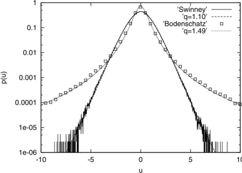
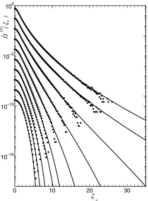
As early as in 1996 Boghosian made the first application of the present formalism to turbulence [16]. That was for plasma. What we shall instead focus on here is fully developed turbulence in normal fluids. Ramos et al advanced in 1999 [10] the possibility of nonextensive statistical mechanics being useful for such systems. The idea was since then further developed by Beck [11] and by the Arimitsu’s [12], basically simultaneous and independently. They proposed theories within which the probability distribution of the velocity differences and related quantities are deduced from basic considerations. We present in Fig. 1 the comparison of Beck’s theoretical results with recent high precision experimental data for Lagrangian and Eulerian turbulences [17]. In Fig. 2 we show an analogous comparison between Arimitsu’s theoretical results and recent computer experimental data.
1e-06 1e-05 0.0001 0.001 0.01 0.1 1
-10 -5 0 5 10
p(u)
u
’Swinney’ ’q=1.10’ ’Bodenschatz’ ’q=1.49’
Fig. 1 – The distributions of differences of velocity in two different experi-ments of fluid turbulence. The solid lines correspond to Beck’s theory [17].
Hadronic jets:
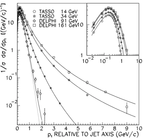
High energy frontal collisions of electron and positron annihilate both and produce relativistic hadronic jets. The distribution of the tranverse momenta of these jets admits, as advanced by Fermi, Feynman, Hagedorn and others, a thermostatistical theoretical approach. Hagedorn’s 1965 theory was q-extended by Bediaga et al in 1999. Their results [13], as well as related ones by Beck [13], compare quite well with the available CERN experimental data, as can be seen in Fig. 3. As important as this is the fact that both Bediaga et al and Beck theories recover a crucial feature of Hagedorn’s scenario, namely that the temperature to be associated with the distributions should
0 10 20 30 10–15
10–10 10–5 100
Π ( ξ )
ξ
(n)
n
n
<
Fig. 2 – The distributions of differences of velocity in numerical ex-periments of fluid turbulence, for typical values ofr/η. The solid lines correspond to the Arimitsu’s theory (see [18] for details). The entire set of theoretical curves has been obtained with a single valueqsen<1.
Hydra viridissima:
Fig. 3 – Distributions of transverse momenta of hadronic jets produced in electron-positron annihilation. The solid lines correspond to the Bediaga-Curado-Miranda theory [13]. To each curve, a different value ofq(in the range
(1,1.2)) is associated. The dashed line corresponds to Hagedorn’s theory using BG statistics(q=1).
Linguistics:
100 101 102 100
101 102 103
Time(min)
<r
2 > (
µ
m
2 )
endo−endo endo−ecto
Fig. 4 – Anomalous diffusion measurements of cells of Hydra viridissima [14]. The dot-dashed line corresponds to normal dif-fusion(q = 1), whereas the solid line corresponds to anomalous superdiffusion associated withq =1.5.
101 102
10−4 10−3 10−2 10−1
|V
x
|(
µ
m/h)
Histogram of velocities
agreement obtained is illustrated with a large set of books by Dickens as shown in Fig. 7. In other words, at large values of the word rank a crossover occurs fromq ≃ 1.9 toq ≃ 1. The reason for this interesting phenomenon is unknown. As a plausible hypothesis, we would like to advance that it might be related to the fact that most authors possibly use the very rare words in a manner which reflects their relatively poor knowledge of their exact meaning. This attitude could make those words to be used slightly uncorrelated with the context within which they are placed. It is however clear that this phenomenon is a very subtle one, and its full elucidation would presumably require very sophisticated analysis.
1 10 100 1000 10000 100000 1000000
1E-9 1E-8 1E-7 1E-6 1E-5 1E-4 1E-3 0.01 0.1
08/03/01 18:30:24
p(r)
r
La Divina Comedia (in Italian, N=101911, V=12865) Decameron (english translation, N=341661, V=14297) William Shakespeare (36 plays, N=890611, V=23182) Don Quijote (in Spanish, N=384590, V=23231) Ulysses (N=140860, V=19495)Dickens (56 books, N=5624548, V=44703) Iliad (in Greek, N=127393, V=20067) Large Corpus: 2750 books in English (N=187832312, V=507369)
Fig. 6 – Zipf plot (frequency of words with rankr) associated with various books as indicated on the figure (N is the total number of words;V is the vocabulary, i.e., the number of different words). See details in [15].
3 A PRIORI DETERMINATION OF THE ENTROPIC INDEX q
1 10 100 1000 10000 100000 1E-8
1E-7 1E-6 1E-5 1E-4 1E-3 0.01 0.1 1
Data: DICKENSFREQS_number Model: Tsallis_2
Chi^2 = 9.9171E-11 R^2 = 0.99986
A 0.07124 ±0.00003
λ 0.40584 ±0.00043
µ 0.0001 ±7.3195E-6 q 1.9 ±0.00036
p(r)
r
Dickens, 56 complete books Number of words: 5624548 Vocabulary suze: 44703
fit (full range)
Fig. 7 – Zipf plot associated with 56 books by Charles Dickens. The solid line corresponds toq =1.9, and the crossover to theq =1 regime at high rankr is visible on the figure. See details in [15].
be used in order to determine without ambiguity the appropriate value(s) ofqfor that system. This crucial question must be answered for the present proposal to be a complete theory, in the sense that it is in principle able to predict the results to be expected in all types of experiments with well defined systems. This question has by now been answered in several important classes of systems. We shall briefly review here two of them, namely low-dimensional maps and long-range many-body classical Hamiltonian systems.
A. Low-dimensional maps
One-dimensional maps:
We consider here one-dimensional dissipative maps of the type
xt+1=f (xt;a, z) (t =0,1,2, . . . ;xt ∈ [xmin, xmax]) , (18)
where a ∈ R is a control parameter such that when it increases for fixed z, it makes the map to become chaotic (we note ac the smallest value of a above which the system can be chaotic;
z ∈ Ris another control parameter which differs essentially froma in the sense that zcontrols the universality class of the chaotic attractor emerging ata = ac(z); the functionf is such that
chaotic and nonchaotic behaviors are possible for the variablex, depending on the values of(a, z). A paradigmatic such map is the so calledz-logistic map, defined as
xt+1=1−a|xt|z(t=0,1,2, . . .;xt ∈ [−1,1]) , (19)
witha∈(0,2]andz >1. The critical valueac(z)(chaos threshold or edge of chaos) monotonically
increases from 1 to 2 whenzincreases from 1 to infinity;ac(2)= 1.401155. . . . Forz =2 this
map is, as well known, isomorphic to Xt+1 ∝ Xt(1 −Xt). The z-logistic maps and several
others have already been studied [22] within the nonextensive scenario. We briefly review here their main properties. Most of these properties have been found heuristically, and no theorems or rigorous results are available. Consequently, we are unable to precisely specify how generic are the properties we are going to describe. We know, however, that wide classes of maps do satisfy them.
Let us first address the sensitivity to the initial conditions. For all values ofa for which the Lyapunov exponentλ1 is nonzero we verify thatq = 1, i.e.,ξ(t )= eλ1t, with λ1 < 0 for most
values ofa < ac, andλ1>0 for most values ofa > ac. However, for the infinite number of values
ofafor whichλ1=0 we verify thatq =1. More precisely, for values ofasuch as those for which
bifurcations occur between finite cycle attractors of say thez-logistic map, we verify the validity of Eq. (15) withq > 1 and λq < 0 (this has been very recently proved [23]). Fora = ac(z)
we verify that ξ(t )exhibits a complex behavior which has, nevertheless, a simple upper bound which satisfies Eq. (15) withq <1 (from now on notedqsen(z), where the subindexsenstands for
sensitivity) andλq(z) >0 (also this has been very recently proved [24]) . For the universality class
of thez-logistic map we verify thatqsen monotonically increases from minus infinity to a value
slightly below unity, whenzincreases from 1 to infinity (qsen(2) =0.2445. . . ). For thez-cercle
and other maps we verify similar behaviors.
Let us now address the attractor inxspacea=ac(z). Its anomalous geometry can be usefully
characterized by the so calledmultifractal functionf (α, z)which typically is defined in the interval αmin(z)≤α≤max (z), and whose maximal value is thefractalorHausdorffdimensiondf(z). For
thez-logistic map universality class we havedf(z) <1, whereas for thez-circle map universality
law, namely [25]
1
1−qsen(z) =
1 αmin(z) −
1 αmax(z)
(∀z) . (20)
This relation has purely geometrical quantities at its right hand member, and a dynamical quantity at its left hand member. It can also be shown that
1
1−qsen(z) =
(z−1)lnαF
lnb (∀z) , (21)
whereαF is one of the two well known Feigenbaum constants, andbis the attractor scaling (b=2
for period-doubling bifurcations;b=2/(√5−1)for cercle maps).
Let us now address the entropy productiondSq(t )/dt. We first make a partition of the interval
[xmin, xmax]intoW nonoverlaping little windows. We place (randomly or not) inside one of those
Wwindows a large numberNof initial conditions, and run the mapttimes for each of these points. We generically verify that theN points spread into the windows, in such a way that we have the set{Ni}(t )(with
W
i=1Ni(t )=N,∀t). With these numbers we can define the set of probabilities
{pi(t )}wherepi(t )≡Ni(t )/N (∀i). We then choose a value forqand calculateSq(t )by using Eq.
(3). We then make an averageSq(t )over a few or many initial windows (see [22,26] for details),
and finally evaluate numerically limt→∞limW→∞limN→∞Sq(t )/t. We verify a very interesting
result [26], namely that this limit isfiniteonly forq =qsen(z); it diverges for allq < qsen(z)and
vanishes for allq > qsen(z). We shall note this limitKqand constitutes a naturalq-generalization
of the Kolmogorov-Sinai entropy. Summarizing,
Kqsen ≡ lim
t→∞ Wlim→∞ Nlim→∞
Sqsen(t )
t . (22)
It is easy to verify, whenever λ1 > 0, that qsen(z) = 1 and that the Pesin identity holds, i.e.,
K1=λ1. A fascinating open question constitutes to find, wheneverλ1 =0 (more specifically for
a =ac(z)), under what circumstances the conjectureKqsen = λqsen could be true,λqsen being the
coefficient appearing in Eq. (15) forq =qsen. We would then have the generalization of the Pesin
identity.
Let us next address another aspect [27] concerning the edge of chaosac(z). We spread now, at
t =0, theN points uniformly within the entire[xmin, xmax]interval, i.e., overalltheW windows,
and follow, as function of time t, the shrinking of the numberW (t ) of windows which contain at least one point (disappearence of the Lebesgue measure on the x-axis); W (0) = W. It can be verified that, for the sequence limW→∞limN→∞, we asymptotically haveW (t ) ∝ 1/t
1
qrel (z)−1,
whereqeq(z) >1 (the subindexrelstands forrelaxation). The entropic indexqrelmonotonically
increases when z increases from 1 to infinity; also, within some range it is verified [27] that 1/[qrel(z)−1] ∝ [1−df(z)]2. We shall now advance a recently established [28] relation between
qrelandqsen.
increases. To be more preciseSqsen(0) = 0 and 0 < Sqsen(∞) < lnqsenW. While t increases,
there are many windows for which Sqsen(t ) overshoots aboveSqsen(∞). We choose the window
for which the overshooting is the most pronounced. AfterSqsen(t ) achieves this peak, it relaxes
slowly towardsSqsen(∞). It does so as 1/t
1
qrel (z,W )−1, whereq
rel(z, W )approaches its limiting value
qrel(z,∞)whileW diverges. The remarkable fact is thatqrel(z,∞)=qrel(z)! More than this, the
approach is asymptotically as follows:
qrel(z)−qrel(z, W )∝
1
Wqsen(z). (23)
This relation is a remarkable connection between the mixing properties, the equilibration (or re-laxing) ones, and the degree of graining (from coarse to fine graining while W increases). We may also say that in some sense Eq. (23) provides a connection between the Boltzmannian and the Gibbsian approaches to statistical mechanics. Indeed, the concept ofqsenis kind of natural within
a typical Boltzmann scenario where individual trajectories in phase space are the ‘‘protagonists of the game’’, whereasqrel is kind of natural within a typical Gibbs scenario where the entire phase
space is to be in principle occupied. Before taking into Eq. (23) theqsen = qrel = 1 particular
case (i.e., the BG-like case), some adaptation is obviously needed; as written in Eq. (23), it is valid only forqsen<1 andqrel >1.
Two-dimensional maps:
We consider here two-dimensional conservative maps of the type
xt+1=fx(xt, yt;a, z)
yt+1=fy(xt, yt;a, z)
(24)
where xt ∈ [xmin, xmax] and yt ∈ [ymin, ymax] with t = 0,1,2, . . .; the control parameter z
characterizes, as for the one-dimensional maps we considered above, the universality class; the control parametera ≥ 0 and we assume that, whileaincreases from zero to its maximum value, the nonnegative Lyapunov exponentλ1monotonically increases from zero to its maximum value.
Since the map is conservative (i.e.,|∂(xt+1, yt+1)/∂(xt, yt)| =1), the other Lyapunov exponent is
−λ1. A paradigmatic such map is the so calledstandard map, defined as follows
yt+1=yt+
a
2π sin(2π xt) (mod1)
xt+1=yt+1+xt =yt +
a
2π sin(2π xt)+xt (mod1)
(25)
as well as itsz-generalization [29], defined as follows
yt+1=yt +
a
2π sin(2π xt)|sin(2π xt)|
z−1 (mod1)
xt+1=yt+1+x1=yt+
a
2π sin(2π xt)|sin(2π xt)|
z−1
+xt (mod1) ,
wherez∈R.
Some (not clearly characterized yet) classes of such maps exhibit for the entropy production
dSq(t )/dt a behavior which closely follows the crossover behavior associated with Eq. (17). Let
us be more precise. We first partition the accessible(x, y)phase inW nonoverlaping little areas (for exampleW little squares), and put a large numberN of initial conditions inside one of those areas. As before, we follow along time the set of probabilities{pi}, with which we calculateSq(t )
for an arbitrarily chosen value ofq. We then average over the entire accessible phase space and obtainSq(t ). Finally we numerically approach the quantitySq(t )≡limW→∞limN→∞Sq(t ).
For large values of a, we verify [30] that S1(t ) asymptotically increases linearly witht, as
expected from the fact thatλ1(a) >0, in agreement with Pesin identity. However, an interesting
phenomenon occurs for increasingly smalla, hence increasingly smallλ1. For smallt (say 0 <
t < < t1(a, z),Sq(t )is linear witht forq =0, and acquires an infinite slope for anyq < 0. For
intermediatet (sayt1(a, z) < < t2(a, z),Sq(t )is linear witht forq = qsen(z) < 1, acquires an
infinite slope forq < qsen(z)and acquires a vanishing slope forq > qsen(z). For large t (say
t > > t2(a, z)),Sq(t )is linear withtforq =1, acquires an infinite slope forq < 1 and acquires
a vanishing slope forq >1. The characteristic timest1(a, z)andt2(a, z)respectively correspond
to the[q = 0] → [q = qsen(z)] and [q = qsen(z)] → [q = 1] crossovers. The remarkable
feature is that, in the limit a → 0, t1(a, z) remains finite whereas t2(a, z) diverges. In other
words, for asymptotically small values ofa, the time evolution ofSq(t )is, excepting for an initial
transient, basically characterized byqsen(z) < 1. This fact opens the possibility for something
similar to occur for Hamiltonian classical systems for which the Lyapunov spectrum tends to zero. This is precisely what occurs when the size of the system increases in the presence of long-range interactions, as we shall see in the next Subsection. Before closing this subsection, let us mention that studies focusing onqrelfor conservative maps are in progress.
B. Long-range many-body classical hamiltonian systems
From the thermodynamical viewpoint it is interesting to classify the two-body interactions (and analogously, of course, the many-body interactions). According to their behavior near the origin, i.e., for r → 0, potentials could be classified as collapsing andnoncollapsing. Collapsing are those which exhibit a minimum atr =0. This minimum can be infinitely deep, i.e., the potential can be singular at r = 0; such is the case of attractive potentials which asymptotically behave as−1/rν withν >0 (e.g., Newtonian gravitation, henceν = 1). Alternatively, the potential at thisr = 0 minimum can be finite, as it is the case of those which behave as −a +br−ν with a >0,b >0 andν <0. Collapsing potentials, especially those of the singular type, are known to exhibit a variety of thermodynamical anomalies.Noncollapsingpotentials are those which exhibit a minimum either at a finite distance (e.g., the Lennard-Jones one, or the hard spheres model or any other model having a cutoff at a finite distancer0) or at infinity (e.g., Coulombian repulsion).
intoshort- andlong-range interactions. Short-range interactions are those whose associated force quickly decreases with distance, for example potentials which exponentially decrease with distance, or classical potentials of the type−1/rαwithα > d,dbeing the space dimension where the system is defined. For classical systems, thermodynamically speaking,short-range interactions correspond to the potentials which are integrable at infinity [33], andlong-range interactions correspond to those which arenotintegrable in that limit, such as those increasing like 1/rα withα <0 (which
belong to theconfining class of potentials, i.e., those which make escape impossible), or those like −1/rα with 0
≤ α/d ≤ 1 (which belong to the nonconfiningclass of potentials, i.e., those which make escape possible). Long-range interactions, especially those of the nonconfining type, are also known to induce a variety of thermodynamical anomalies. From the present standpoint a particularly complex potential is Newtonian gravitation (corresponding toα = 1 andd = 3). Indeed, it is both singular at the origin, and long-ranged since 0< α/d=1/3<1.
In this Section we address an important case, namely that of nonsingular attractive long-range two-body interactions in ad-dimensionalN-body classical hamiltonian system withN >>1. Such systems are being actively addressed in the literature by many authors (see [31,32] and references therein). As an illustration of the thermodynamical anomalies that long-range interactions produce, we shall focus on thed-dimensional simple hypercubic lattice with periodic boundary conditions, each site of which is occupied by a classical planar rotator. All rotators are coupled two by two as indicated in the following Hamiltonian:
H=
N
i=1
L2i
2 +
i=j
1−cos(θi−θj)
rijα (θi ∈ [0,2π];α≥0) . (27)
The distance (in crystal units) between any two sites is the shortest one taking into account the periodicity of the lattice. Ford =1, it is rij = 1,2,3, . . .; ford = 2, it isrij1,
√
2,2, . . .; for d =3, it isrij =1,
√
2,√3,2, . . .; and so on for higher dimensions. We have written the potential term in such a way that it vanishes in all cases for the fundamental state, i.e.,θi =θ0(∀i), where,
without loss of generality, we shall considerθ0=0 for simplicity. Also without loss of generality
we have considered unit moment of inertia and unit first-neighbor coupling constant. It is clear that, excepting for the inertial term, the present model is nothing but the classicalXY ferromagnet. The casesα =0 andα→ ∞respectively correspond to the so called HMF model [31] (all two-body couplings have the same strength), and to the first-neighbor model. For BG statistical mechanics to be applicable without further considerations, it is necessary that the potential be integrable, i.e.,
∞ 1 dr r
d−1r−α <
following one instead:
N1/d
1
dr rd−1r−α, (28)
which, in theN → ∞limit, converges forα/d >1 and diverges otherwise. It is in fact convenient to introduce the quantity
N ≡1+d N1/d
1
dr rd−1r−α = N
1−α/d
−α/d
1−α/d . (29)
N equalsN forα =0, and, forN → ∞, diverges likeN1−α/dfor 0< α/d, diverges like lnN for α/d=1, and is finite forα/d >1, being unity in the limitα/d → ∞. In general, the energy per particle scales withN; in other words, the energy is nonextensive for 0 ≤α/d ≤1. To make the problem artificially extensive even forα/d ≤1, the Hamiltonian can be written as follows:
H′=
N
i=1
L2i
2 +
1
N
i=j
1−cos(θi −θj)
rijα . (30)
The rescaling of the potential of this model is more properly taken into account byi=jrij−α [34] rather than byN, but since theirN → ∞asymptotic behaviors coincide, we can as well useN as introduced here. The original (Eq. (27)) and rescaled (Eq. (30)) versions of this model are completely equivalent (see [32]) and lead to results that can be easily transformed from one to the other version. To make easier the comparison of results existing in the literature, we shall from now on refer to the rescaled version (30).
Theα =0 model (HMF) clearly isd-independent and is paradigmatic of what happens for any αsuch that 0 ≤α/d <1. When isolated (microcanonical ensemble) theα/d=0 model exhibits a second-order phase transition atu≡U/N =0.75, whereUis its total energy andN → ∞. This critical valueucsmoothly increases withα/dapproaching unity. Dynamical and thermodynamical
anomalies exist in both ordered and disordered phases, respectively foru < ucandu > uc. Let us
discuss some anomalies foru > uc, then some foru < uc, and finally show that these anomalies
on both sides ofucare in fact connected.
The Lyapunov spectrum is made by couples of real quantities that are equal in absolute value and opposite in sign, whose sum vanishes in accordance with the Liouville theorem. The sum of the positive values equals the Kolmogorov-Sinai entropy, in accordance with the Pesin theorem. If the maximal Lyapunov exponent vanishes, the entire spectrum vanishes, and no exponentially quick sensitivity to the initial conditions is possible.
We address first the caseu > uc. For the Hamiltonian of rotors we are interested in (Eq. (30)),
the maximal Lyapunov exponentλ˜maxscales, for largeN, like
˜
λmax ∼ l(u, α, d)
wherel(u, α, d)is some smooth function of its variables, andκ(α/d)decreases from 1/3 to zero whenα/dincreases from zero to unity;κremains zero for all values ofα/dabove unity, consistently with the fact that λ˜max is positive in that region. In other words, above the critical energy, the sensitivity to the initial conditions is exponential forα/d >1, and subexponential (possibly power like) for 0≤α/d≤1.
We address now the case 0 < u < uc, and focus especially on the region slightly below the
critical valueuc(e.g.,u=0.69 for theα=0 model). For 0≤α/d ≤1, at least two (and possibly
only two with nonzero measure) important basins exist in the space of the initial conditions: one of them contains the Maxwellian distribution of velocities, the other one contains the water-bag (as well as the double water-bag) distibution of velocities. When the initial conditions belong to the Maxwellian basin, the system relaxes quickly onto the BG equilibrium distribution (strictly speaking, we do not have this numerical evidence but a weaker one, namely that the marginal probability of one-rotator velocities tends to the Maxwellian one when N → ∞). When the initial conditions belong to the other basin, it first relaxes quickly to an anomalous, metastable (quasi-stationary) state, and only later, at a crossover time τ, starts slowly approaching the BG equilibrium. The crossover time diverges with N forα = 0 [36]. It has been conjectured [35] that it might in general diverge likeτ ∼ N. It has been recently established [37] that, ford = 1 and fixedN,τ exponentially vanishes withα approaching unity. All these features are consistent with the conjectureτ ∼N, which might well be true. During the metastable state, the one-particle distribution of velocities is clearly non Gaussian, and in fact it seems to approach the distribution of velocities typical of nonextensive statistical mechanics for q > 1. This anomalous behavior reflects on the sensitivity to the initial conditions. The maximal Lyapunov exponentλ˜maxremains
during long time, in fact untilt ∼τ, at a low value and then starts approaching a finite value. This low value scales like 1/Nκ′(α/d). The remarkable feature which has been observed [38,39] for the
d =1 model is thatκ′ =κ/3 for all values ofα. The anomalies above and below the critical point become thus intimately related.
The whole scenario is expected to hold for large classes of models, including the classical n-vector ferromagnetic-like two-body coupled inertial rotors (n=2 being the present one,n=3 the Heisenberg one, n → ∞the spherical one, etc). For all of them, in the isolated situation, we expect (i) at the disordered phase, that the maximal Lyapunov decreases with N with the exponent κ(α/d, n) (it is yet unclear whether this exponent depends on n or not); (ii) at the ordered phase, and starting from initial conditions within a finite basin including the water-bag, that a metastable state exists with non BG (possiblyq-type) distribution associated with a maximal Lyapunov exponent which decreases withN with the exponentκ(α/d)/3. In these circumstances, forα/d≤1 (nonextensive systems), the limN→∞limt→∞ordering is expected to yield the usual BG
equilibrium, whereas the limt→∞limN→∞ordering yields a non BG (meta)equilibrium, possibly of
the BG one, as known since long.
4 CONCLUSIONS
We have presented some of the main peculiarities associated with nonextensive systems. Most of the paradigmatic behaviors are expected to become (or have been shown to become) power laws instead of the usual exponentials:
(i) the sensitivity to the initial conditions is given by ξ = eqλqt (typicallyq ≤ 1 at the edge of
chaos);
(ii) the finite entropy production (Kolmogorov-Sinai entropy like) occurs only forSq(withq ≤1,
the same as above);
(iii) the relaxation towards quasi-stationary or (metaequilibrium) states, or perhaps from these to the terminal equilibrium states, may occur throughe−qt /τq (typicallyq ≥1);
(iv) the stationary, (meta)equilibrium distribution for thermodynamically large Hamiltonian sys-tems may be given bypi ∝ e−
β′ǫi
q (typicallyq ≥ 1, possibly the same as just above, at least
for some cases).
The two-dimensional conservative maps exhibit, in the vicinity of integrability and at inter-mediate times, features very similar to those observed in one-dimensional dissipative maps at the edge of chaos. The intermediate stage has a duration which diverges when the control parameters approach values where the system is close to integrability. Isolated classical Hamiltonian sys-tems behave similarly to low-dimensional conservative maps, 1/N playing a role analogous to the distance of the control parameters to their values where integrability starts.
The scenario which emerges is that sensitivity and entropy production properties are related to one and the same value ofqsen≤ 1 (also related toαminandαmaxof some multifractal function),
whereas the relaxation and (meta)equilibrium properties are related to (possibly one and the same) value of qrel ≥ 1 (also related to the Hausdorff dimension of the same multifractal function).
These two sets of properties are quite distinct and generically correspond to distinct values ofq (namely,qsenandqrel). It happens that for the usual, extensive, BG systems they coincide providing
qsen=qrel =1, which might sometimes be at the basis of some confusion. In all cases, once the
microscopic dynamics of the systems is known, it is in principle possible to determinea prioriboth qsenandqrel(as well as the connection among them and with the chosen graining, as illustrated in
Eq. (23)). We have here shown how this is done for simple systems. This type of calculation of
ACKNOWLEDGEMENTS
I thank I. Bediaga, E.M.F. Curado, J. Miranda, C. Beck, T. and N. Arimitsu, A. Upadhyaya, J.-P. Rieu, J.A. Glazier and Y. Sawada and M.A. Montemurro for kindly providing and allowing me to use the figures that are shown here. I also thank CNPq, PRONEX and FAPERJ (Brazilian agencies) and FCT (Portugal) for partial financial support. Finally, I am grateful to B.J.C. Cabral, who provided warm hospitality at the Centro de Fisica da Materia Condensada of Universidade de Lisboa, where this work was partially done.
RESUMO
Revisamos sumariamente o estado presente da mecânica estatística não-extensiva. Focalizamos em (i) as
equacões centrais do formalismo; (ii) as aplicações mais recentes na física e em outras ciências, (iii) a
determinaçãoa priori(da dinâmica microscópica) do índice entrópicoq para duas classes importantes de
sistemas físicos, a saber, mapas de baixa dimensão (tanto dissipativos quanto conservativos) e sistemas
clássicos hamiltonianos de muitos corpos com interações de longo alcance.
Palavras-chave: mecânica estatística não extensiva, entropia, sistemas complexos.
REFERENCES
[1]Tsallis C.1988. Possible generalization of Boltzmann-Gibbs Statistics. J Stat Phys 52: 479-487.
[2]Curado EMF and Tsallis C.1991. Generalized statistical-mechanics – connection with thermody-namics. J Phys A-Math Gen 24: L69-L72. 1991. Correction 24: 3187-3187. 1992. Correction 25: 1019-1019.
[3]Tsallis C, Mendes RS and Plastino AR.1998. The role of constraints within generalized nonextensive statistics. Physica A 261: 534-553.
[4] Salinas SRA and Tsallis C.1999. Non extensive Statistical Mechanics and Thermodynamics, Braz J Phys 29U4-U4. Abe S and Okamoto Y.2001. Nonextensive Statistical Mechanics and Its Applications, Series Lectures Notes in Physics. Springer, Berlin. Grigolini P, Tsallis C and West BJ.2002. Classical and Quantum Complexity and Nonextensive Thermodynamics, Chaos Soliton Fract
13: 367-370. Kaniadakis G, Lissia M and Rapisarda A. 2002. Nonextensive Thermodynamics and Physical Applications. Physica A 305. Gell-Mann M and Tsallis C.2002. Nonextensive Entropy-Interdisciplinary Applications. Oxford University Press, Oxford. In preparation.
[5]http://tsallis.cat.cbpf.br/biblio.htm.
[6]Tsallis C, Levy SVF, Souza AMC and Maynard R.1995. Statistical-mechanical foundation of the ubiquity of Levy distributions in nature; Phys Rev Lett 75: 3589-3593.Tsallis C, Levy SVF, Souza AMC and Maynard R.1996. Statistical-mechanical foundation of the ubiquity of Levy distributions
Zanette DH and Alemany PA.1996. Thermodynamics of anomalous diffusion – Reply. Phys Rev
Lett 77: 2590-2590. Buiatti M, Grigolini P and Montagnini A.1999. Dynamic approach to the thermodynamics of superdiffusion. Phys Rev Lett 82: 3383-3387. Prato D and Tsallis C.1999. Nonextensive foundation of Levy distributions. Phys Rev E 60:2398-2401 Part B.
[7]Bak P.1996. How Nature Works: The Science of self-organized criticality. Springer-Verlag, New York, 212 pp.
[8]Mandelbrot BM.1982. The Fractal Geometry of Nature. W.E. Freeman, New York, 468 pp.
[9]Gell-Mann M.1999. The Quark and the Jaguar: Adventures in the Simple and the Complex. W.H. Freeman, New York, 392 pp.
[10]Ramos FM, Rosa RR and Rodrigues-Neto C.1999. Cond-mat 9907348. Ramos FM, Rodrigues-Neto C and Rosa RR.2000. cond-mat/0010435.Ramos FT, Rosa RR, Neto CR, Bolzan MJA, Sa
LDA and Campos-Velho HFC.2001. Non-extensive statistics and three-dimensional fully developted
turbulence. Physica A 295: 250-253. Rodrigues-Neto C, Zanandrea A, Ramos FM, Rosa RR, Bolzan MJA and Sa LDA.2001. Multiscale analysis from turbulent time series with wavelet transform.
Physica A 295: 215-218. Campos-Velho HF, Rosa RR, Ramos FM, Pielke RA, Degrazia GA, Rodrigues-Neto C and Zanandrea Z.2001. Multifractal model for eddy diffusivity and
counter-gradient term in atmospheric turbulence Physica A 295: 219-223.
[11]Beck C.2000. Application of generalized thermostatistics to fully developed turbulence. Physica A 277: 115-123.Beck C.2001. On the small-scale statistics of Lagrangian turbulence. Phys Lett A 287: 240-244. Shivamoggi BK and Beck C.2001. A note on the application of non-extensive statistical mechanics to fully developed turbulence. J Phys A – Math Gen 34: 4003-4007. Beck C, Lewis GS and Swinney HL.2001. Measuring nonextensitivity parameters in a turbulent Couette-Taylor flow.
Phys Rev E 63: 035303.
[12]Arimitsu T and Arimitsu N.2000. Analysis of fully developed turbulence in terms of Tsallis statistics. Phys Rev E 61: 3237-3240.Arimitsu T and Arimitsu N.2000. Tsallis statistics and fully developed turbulence. J Phys A-Math 33: L235-L241. Arimitsu T and Arimitsu N.2001. Tsallis statistics and fully developed turbulence. Corrigenda (Vol 33: L235-L241, 2000.) J Phys A-Math 34: 673-674. Arimitsu T and Arimitsu N.2001. Analysis of turbulence by statistics based on generalized entropies.
Physica A 295: 177-194.
[13]Bediaga I, Curado EMF and Miranda J.2000. A non-extensive thermodynamical equilibrium approach in e(+) e(-)→hadrons. Physica A 286: 156-163. Beck C.2000. Non-extensive statistical mechanics and particle spectra in elementary interactions. Physica A 286: 164-180.
[14]Upadhyaya A, Rieu J-P, Glazier JA and Sawada Y.2001. Anomalous diffusion and non-Gaussian velocity distribution of Hydra cells in cellular aggregates. Physica A 293: 549-558.
[15]Montemurro MA.2001. Beyond the Zipf-Mandelbrot law in quantitative linguistics. Physica A 300: 567-578.
[17]Beck C. 2001. Dynamical foundations of nonextensive statistical mechanics. Phys Rev Lett 87: 180601.
[18]Arimitsu T and Arimitsu N.2002. PDF of velocity fluctuation in turbulence by a statistics based on generalized entropy. Physica A 305: 218-226.
[19]Tsallis C and Bukman DJ.1996. Anomalous diffusion in the presence of external forces: Exact time-dependent solutions and their thermostatistical basis. Phys Rev E 54: R2197-R2200.
[20]Denisov S.1997. Fractal binary sequences: Tsallis thermodynamics and the Zipf law. Phys Lett A 235: 447-451.
[21]Plastino AR and Plastino A. 1993. Stellar polytropes and Tsallis entropy. Phys Lett A 174: 384-386.
[22] Tsallis C, Plastino AR and Zheng W-M. 1997. Power-law sensitivity to initial conditions – New entropic representation. Chaos Soliton Fract 8: 885-891. Costa UMS, Lyra ML, Plastino AR and Tsallis C.1997. Power-law sensitivity to initial conditions within a logisticlike family of
maps: Fractality and nonextensivity. Phys Rev E 56: 245-250.Lyra ML.1998. Weak chaos: Power-law sensitivity to initial conditions and nonextensive thermostatistics. Ann Rev Com Phys. 6: 31-58, Stauffer D.(Ed) World Scientific, Singapore. 31 pp. Tirnakli U, Tsallis C and Lyra ML.1999.
Circular-like maps: sensitivity to the initial conditions, multifractality and nonextensivity. Eur Phys J B 11: 309-315. Tirnakli U.2000. Asymmetric unimodal maps: Some results from q-generalized bit cumulants. Phys Rev E 62: 7857-7860 Part A.DaSilva CR, daCruz HR and Lyra ML.1999. Low-dimensional, non-linear dynamical systems and generalized entropy. Braz J Phys 29: 144-152. Tirnakli U, Ananos GFJ and Tsallis C.2001. Generalization of the Kolmogorov-Sinai entropy:
logistic-like and generalized cosine maps at the chaos threshold. Phys Lett A 289: 51-58.Yang J and Grigolini P.1999. On the time evolution of the entropic index. Phys Lett A 263: 323-330.
[23]Baldovin F and Robledo A.cond-mat/0205356.
[24]Baldovin F and Robledo A.cond-mat/0205371.
[25]Lyra ML and Tsallis C.1998. Nonextensivity and multifractality in low-dimensional dissipative systems. Phys Rev Lett 80: 53-56.
[26]Latora V, Baranger M, Rapisarda A. and Tsallis C.2000. The rate of entropy increase at the edge of chaos. Phys Lett A 273: 97-103.
[27]de-Moura FABF, Tirnakli U and Lyra ML.2000. Convergence to the critical attractor of dissipative maps: Log-periodic oscillations, fractality and nonextensivity. Phys Rev E 62: 6361-6365 Part A.
[28]Borges EP, Tsallis C, Ananos GFJ and Oliveira PMC.cond-mat/0203348.
[29]Baldovin F and Tsallis C.2001. Unpublished.
[30]Baldovin F, Tsallis C and Schulze B.2001. cond-mat/0108501.
[32]Anteneodo C and Tsallis C.1998. Breakdown of exponential sensitivity to initial conditions: Role of the range of interactions. Phys Rev Lett 80: 5313-5316.
[33]Fisher ME.1964. The free energy of a macroscopic system. Arch Rat Mech Anal 17: 377-410. Fisher ME.1965. Bounds for derivatives of free energy and pressure of a hard-core system near close
packing.J Chem Phys 42: 3852-&Fisher ME.1965. Correlation functions and coexistence of phases. J Math Phys 6: 1643-&Fisher ME and Ruelle D.1966. Stability of many-particle systems. J Math Phys 7: 260-&Fisher ME and Lebowitz JL.1970. Asymptotic free energy of a system with periodic boundary conditions. Commun Math Phys 19: 251-&
[34]Tamarit FA and Anteneodo C.2000. Rotators with long-range interactions: Connection with the mean-field approximation. Phys Rev Lett 84: 208-211.
[35]Tsallis C.2000. Communicated at the HMF Meeting. Universita di Catania 6-8 September.
[36]Latora V, Rapisarda A and Tsallis C.2001. Non-Gaussian equilibrium in a long-range Hamiltonian system. Phys Rev E 64: 056134.
[37]Campa A, Giansanti A and Moroni D.2002. Metastable states in a class of long-range Hamiltonian systems. Physica A 305: 137-143.
[38]Latora V, Rapisarda A and Tsallis C.2002. Fingerprints of nonextensive thermodynamics in a long-range Hamiltonian system. Physica A 305: 129-136.
[39]Cabral BJC and Tsallis C.cond-mat/0204029.
![Fig. 4 – Anomalous diffusion measurements of cells of Hydra viridissima [14]. The dot-dashed line corresponds to normal dif-fusion (q = 1), whereas the solid line corresponds to anomalous superdiffusion associated with q = 1.5.](https://thumb-eu.123doks.com/thumbv2/123dok_br/15969256.687037/8.918.186.661.178.561/anomalous-diffusion-measurements-viridissima-corresponds-corresponds-superdiffusion-associated.webp)


