Bishoksan Kafle
Modeling Assembly Program with
Constraints
A Contribution to WCET Problem
Dissertação para obtenção do Grau de Mestre em Lógica Computacional
Orientador: Pedro Barahona, Professor Catedrático,
Faculdade de
Ciências e
Tecnologia,
Universidade Nova de Lisboa
Co-orientador: Franck Cassez, Principal Researcher,
NICTA
Júri:
Presidente: Prof. Doutor José Júlio Alferes Arguente: Prof. Doutor Luis Gomes Vogal: Prof. Doutor Pedro Barahona
First, I would like to thank my supervisor Prof. Pedro Barahona for his kind supervision of this thesis. Without his scientific virtue, wide-knowledge, support and advices this thesis would have never been possible. I am also thankful for his great patience and understanding. My sin-cere gratitude to my co-supervisor Dr. Franck Cassez, NICTA, Australia for kind supervision, guidance, valuable advices and for the original proposal of the thesis.
I would like to thank the EMCL consortium for the two year scholarship and for giving me a chance to learn from the best. I would also like to thank all the staff members who guided me during my studies here in Europe.
I want to thank all of my friends in Dresden, Lisbon, Bolzano and Vienna who have made my these two years as one of the most beautiful periods in my life from all perspectives. I like to thank Sudeep Ghimire for proof-reading and for being there whenever I was in need.
Model checking with program slicing has been successfully applied to compute Worst Case Execution Time (WCET) of a program running in a given hardware. This method lacks path feasibility analysis and suffers from the following problems: The model checker (MC) explores exponential number of program paths irrespective of their feasibility. This limits the scalability of this method to multiple path programs. And the witness trace returned by the MC corre-sponding to WCET may not be feasible (executable). This may result in a solution which is not tight i.e., it overestimates the actual WCET.
This thesis complements the above method with path feasibility analysis and addresses these problems. To achieve this: we first validate the witness trace returned by the MC and generate test data if it is executable. For this we generate constraints over a trace and solve a constraint satisfaction problem. Experiment shows that33%of these traces (obtained while computing WCET on standard WCET benchmark programs) are infeasible. Second, we use constraint solving technique to compute approximate WCET solely based on the program (without tak-ing into account the hardware characteristics), and suggest some feasible and probable worst case paths which can produce WCET. Each of these paths forms an input to the MC. The more precise WCET then can be computed on these paths using the above method. The maximum of all these is the WCET. In addition this, we provide a mechanism to compute an upper bound of over approximation for WCET computed using model checking method. This effort of com-bining constraint solving technique with model checking takes advantages of their strengths and makes WCET computation scalable and amenable to hardware changes. We use our tech-nique to compute WCET on standard benchmark programs from M¨alardalen University and compare our results with results from model checking method.
1 INTRODUCTION 1
1.1 Motivation . . . 1
1.2 Structure of this work . . . 2
1.3 Contributions . . . 3
2 TIMING ANALYSIS TECHNIQUES AND WCET 5 2.1 Overview of Timing Analysis Techniques . . . 6
2.2 WCET . . . 6
2.2.1 WCET Challenges . . . 7
2.2.2 WCET Methods and Tools . . . 8
2.3 Previous Work . . . 9
2.3.1 IPET . . . 11
2.4 General Consideration . . . 11
3 CONSTRAINTS AND CONSTRAINT SOLVERS 13 3.1 Constraint Satisfaction Problem (CSP) . . . 13
3.2 Constraint Satisfaction Optimization Problem (CSOP) . . . 14
3.3 Constraint Solvers . . . 14
3.3.1 Complete solvers . . . 14
3.3.2 Incomplete solvers . . . 15
3.4 Constraint programming . . . 16
3.4.1 Variable . . . 17
3.4.2 Constraints . . . 17
3.4.3 Search . . . 18
3.5 Partial Conclusion . . . 20
4 PATH FEASIBILITY ANALYSIS 21 4.1 Some assumption about the program (path) . . . 22
4.2 Path Based Analysis . . . 22
4.3 Extracting Path Constraints . . . 23
4.3.1 Modeling Register, Stack and Memory . . . 23
4.3.2 Maintaining Version for the Variables . . . 24
4.3.3 Updating Arrays . . . 26
4.3.4 Constraints Generation Algorithm . . . 27
4.4 Constraint Solving . . . 29
4.5 Experiment and Results . . . 29
5.1.1 Subset of ARM Assembly Language . . . 31
5.1.2 Subset ofCLanguage . . . 32
5.2 Decompilation Phases . . . 33
5.2.1 Reconstruct CFG from Assembly Code . . . 34
5.2.1.1 Partitioning assembly instructions into basic blocks . . . 35
5.2.1.2 CFG from List of Basic Blocks . . . 36
5.2.2 Loops . . . 37
5.2.3 HLL Code Generation . . . 37
5.2.3.1 Generating Code for a Basic Block . . . 38
5.2.3.2 Generating Code from Control Flow Graphs . . . 38
5.3 Mapping between Assembly Language and HLL . . . 40
5.4 Partial Conclusion . . . 41
6 MODELING HLL WITH CONSTRAINTS 43 6.1 Transformation of HLL to CPM . . . 44
6.1.1 Rewriting Rules for different kinds of instructions . . . 44
6.1.1.1 Declaration . . . 44
6.1.1.2 Assignments . . . 46
6.1.1.3 Loop statements . . . 46
6.1.1.4 Conditional Statement . . . 48
6.1.1.5 Special case: Array assignment . . . 50
6.1.1.6 Code Block . . . 51
6.1.1.7 Basic Block Timing, Optimization function and Search . . . 51
6.1.2 Labeling . . . 51
6.1.3 Rules for Generating Labeling Function . . . 54
6.2 Partial Conclusion . . . 55
7 WCET COMPUTATION 57 7.1 OVERVIEW OF THE METHOD AND TOOL CHAIN . . . 57
7.2 Experimental Results . . . 60
7.2.1 Comments on the Results . . . 61
7.3 Comparison between two WCET computation approaches . . . 61
7.3.1 Comments on the Comparison . . . 62
7.4 Paths Study . . . 62
7.5 Partial Conclusion . . . 63
8 CONCLUSIONS AND FUTURE WORKS 65
REFERENCES 67
2.1 Basic notions concerning timing analysis of systems. . . . 5
2.2 WCET calculation methods. . . . 10
3.1 An example of CP model for a feasible solution in Comet . . . 17
3.2 An example of CSP in Comet . . . 18
4.1 An example of a path in assembly language . . . 28
4.2 The system of constraints for the path in figure 4.1. . . 29
5.1 A decompiler . . . 31
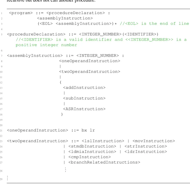
5.2 Formal Grammar of Assembly Language handled . . . 32
5.3 An example of source program: fib-O0 . . . 34
5.4 Partition of program into basic blocks . . . 36
5.5 CFG of fib-O0. . . 37
5.6 Code generation for BBs except for transfer of control instructions . . . 38
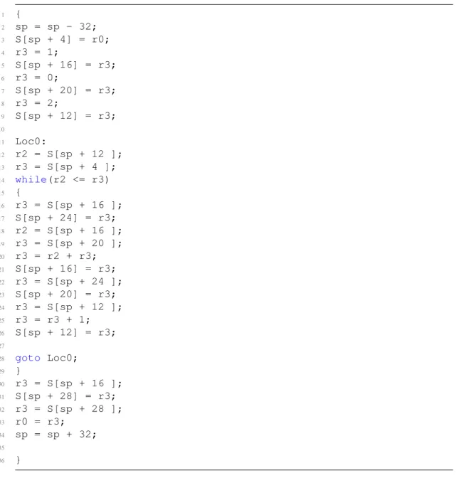
5.7 Complete HLL code for fib-O0 . . . 39
5.8 Complete HLL optimized code for fib-O0. . . 40
7.1 Tool Chain Overview(Aprox. WCET Tool) . . . 58
7.2 Code to obtain worst case paths . . . 59
7.3 Tool Integration with Cassez et. al WCET Tool. . . 59
4.1 Path Feasibility Results . . . 30
Chapter
1
INTRODUCTION
”The best way to predict the future is to invent it.” Alan Kay
Hard real-time systems are those that have crucial deadlines. Typical examples of real-time sys-tems include defense and space syssys-tems, embedded automotive electronics, air traffic control systems, command control systems etc. They are composed of a set of tasks and are charac-terized by the presence of a processor running application specific dedicated software. Here, a task may be a unit of scheduling by an operating system, a subroutine, or some other software unit. In these systems, the correctness of the system behavior depends not only on the logical results of the computations, but also on the physical instant at which these results are produced. So each real-time task has to be completed within a specified time frame.
In order to schedule these systems, we need to know some bounds about execution times of each task i.e. the worst-case execution-time (WCET). These bounds are needed for allocating the correct CPU time to the tasks of an application. They form the inputs for schedulability tools, which test whether a given task set is schedulable (and will thus meet the timing re-quirements of the application) on a given target system. Together with schedulability analysis, WCET analysis forms the basis for establishing confidence into the timely operation of a real-time system [1]. WCET analysis does so by computing (upper) bounds for the execution real-times of the tasks in the system.
This chapter presents the motivation behind this work, lists the contributions we made and presents the overall structure of the thesis.
1.1
Motivation
There are two main classes of methods for computing WCET [2]: Testing/Measurement and Verification based methods. But only the verification based methods (also known as static methods) are guaranteed to produce safe WCET [3]. Two different kinds of techniques are predominant in static methods, namely, Integer Linear Programming(ILP) based and Model Checking based.
inferred automatically. Hereby, the WCET is computed by solving a maximum cost circulation problem in this CFG. Each edge is associated with a certain cost for executing it. The algorithm implemented in these tools use both the program and the hardware specification to compute the CFG fed to the ILP solver. The architecture of the tool is thus monolithic i.e., it is not easy to add support for a new hardware. But these techniques are fast and can handle large programs [4]. They implement implicit path enumeration technique (IPET) and this considerably simpli-fies path analysis [5].
On the other hand, the model checking based techniques presented in [3] rely on the fully automatic method to compute a CFG(without user annotations). It describes the model of the hardware as a product of timed automata (independently of the program). The model of the program running on a hardware is obtained by synchronizing the program with the model of the hardware. Computing WCET is then reduced to a reachability problem on the synchro-nized model and solved using the real time model checker UPPAAL1. These techniques [3, 4] are slower and perform better for simplified programs. But allow easy integration of complex hardware models such as cache and pipelines.
Considerable amount of works have been done on both tasks [2, 3, 4, 5, 6], but each of them usually misses the aspect of the other. In this thesis, we purpose a technique which is a com-bination of these two to take advantage of their strengths and make WCET computation tech-niques scalable and amenable to changes. The idea behind this is to use ILP based techtech-niques for path analysis and model checking based techniques for integration of complex hardware models.
To achieve this, we compute approximate WCET solely based on the program (only consider-ing clock cycles for each instruction from its manual) without takconsider-ing into account the hardware characteristics (cache and pipelines) using Constraint Programming (CP) instead of ILP. Based on this approximate value, we propose some feasible and most probable worst case paths to model checking based techniques. Model checking technique then combines the hardware model to this program path suggested by CP and computes the precise WCET. In doing so, we get rid of monolithicity problem of ILP based techniques and the scalability issues of the model checking techniques and yet keeping intact their strengths.
1.2
Structure of this work
The rest of this work is organized as follows. The next chapter provides an overview of timing analysis techniques and WCET. Chapter 3 provides some background knowledge about con-straints and constraint solvers. Chapter 4 deals with the path analysis, mainly, the algorithms and results of path validation. Chapter 5 discusses briefly about high-level language gener-ation from assembly language. Similarly, chapter 6 presents some rewriting rules to obtain Constraint Programming Model (CPM) of a high level language. Chapter 7 explains about our technique of computing approximate WCET. Next, chapter 8 concludes this thesis, by pro-viding a summary of this work, and highlighting some possible research directions for future work. Finally, Appendix A is a supplementary chapter which presents CPM of some bench-mark programs used to compute WCET.
1
1.3
Contributions
Chapter
2
TIMING ANALYSIS TECHNIQUES
AND WCET
”Joy in looking and comprehending is nature’s most beautiful gift.” Albert Einstein
This chapter presents some background knowledge about WCET, its challenges and some methods and tools for computing WCET. The knowledge of the maximum time consumption of each program or task or piece of code is a prerequisite for analyzing the worst-case timing behavior of a real-time system and for verifying its temporal correctness. This maximum time needed by each program is assessed by means of WCET analysis. Figure 2.1 taken from [2] depicts several relevant properties of a real-time task. The lower curve represents a subset of measured executions. Its minimum and maximum are the minimal observed execution times and maximal observed execution times, resp. The darker curve, an envelope of the former, rep-resents the times of all executions. Its minimum and maximum are the best-case and worst-case execution times, resp., abbreviated BCET and WCET.
Figure 2.1:Basic notions concerning timing analysis of systems.
different behavior of the environment. The set of all execution times is shown as the upper curve. The shortest execution time is called the BCET, the longest time is called the WCET. In most cases the state space is too large to exhaustively explore all possible executions and thereby determine the exact worst-case and best-case execution times. Timing analysis is a process of deriving execution-time bounds or estimates. A tool that derives bounds or estimates for the execution times of application tasks is called a timing-analysis tool.
2.1
Overview of Timing Analysis Techniques
Timing analysis attempts to determine bounds on the execution times of a task when executed on a particular hardware. The time for a particular execution depends on the path through the task taken by control (referred to as the program path analysis problem) and the time spent in the statements or instructions on this path on this hardware (referred to as micro-architectural modeling). Both these aspects need to be studied well in order to provide a solution to this problem. The focus of this thesis is on the program path analysis problem. The structure and the functionality (i.e., what the program is computing) of a program determines the actual paths taken during its execution. Any information regarding these helps in deciding which program paths are feasible and which are not. While some of this information can be automatically in-ferred from the program, this is a difficult task in general (e.g., regarding the information about functionality of a program).
Accordingly, the determination of execution-time bounds has to consider the potential control-flow paths and the execution times for this set of paths. A modular approach to the timing-analysis problem splits the overall task into a sequence of subtasks. Some of them deal with properties of the control flow, others with the execution time of instructions or sequences of instructions on the given hardware. Many of today’s approaches to WCET analysis demand that the programmer provide information about (in)feasible execution paths of the code to be analyzed. This path information is described at the high-level language interface. On the other hand, the actual computation of WCET, that uses this path information, takes place at the machine-language level, where the execution times of basic actions can be accurately modeled. Today’s practical approaches to WCET analysis therefore have to bridge the gap between these two different representation levels. This makes timing analysis difficult and interesting as a research topic. The progress in this field has led to a number of techniques and tools which will be discussed in the next sections.
2.2
WCET
WCET analysis computes upper bounds for the execution times of programs for a given appli-cation, where theexecution timeof aprogram is defined as the time it takes the processor to execute thatprogram. Formally, it can be defined as [3]:
Definition 2.1 The WCET of a programPon a hardwareH, represented asW CET(P, H), is the maximum execution time(time(H, P, d)) ofPonHfor all input datad, wheretime(H, P, d) is the execution time ofP for input datadonH.
Mathematically,
W CET(P, H) = max
d∈D time(H, P, d),∀d
programs always terminate; recursion is not allowed or explicitly bounded as are the iteration counts of loops. A reliable guarantee based on the worst-case execution time of a task could easily be given if the worst-case inputs for the task were known. Unfortunately, in general the worst-case inputs are not known and are hard to derive. We should bear in mind the following points regarding the WCET [1]:
1. WCET analysis computes upper bounds for the WCET, i.e. it does not guarantee to return the WCET exactly.
2. The WCET bound computed for a piece of code is application- dependent , i.e., a single piece of code may have different WCETs, and thus WCET bounds in different applica-tion contexts.
3. WCET analysis assesses the duration that the processor is actually executing the ana-lyzed piece of code, i.e. assuming non-preemptive execution. It is important to note that the results of WCET analysis do not include waiting times due to preemption, blocking, or other interference.
4. WCET analysis is hardware-dependent. WCET analysis therefore has to model the fea-tures of the target hardware on which the code is supposed to execute.
In order to make real-time systems temporally predictable and to keep the price of such systems reasonable, the computed WCET has to be [1, 3] :
1. safe i.e., it must not under-estimate the worst case, and
2. tight otherwise either the set of tasks are wrongly declared non schedulable or the cost has to be paid in order to compensate with the pessimism.
LetC be the computed WCET andM be the measured WCET on the real platform for some program P, then the over approximation is given by the formula: (C −M)/M ∗100. The computed WCET is considered tight when the difference betweenC andM is lesser or equal to some epsilon(ǫ).
2.2.1 WCET Challenges
Computing the WCET of a program is a challenging and difficult task. It is usually a very hard problem and there are several factors which are responsible for this [1, 3] :
1. WCET analysis has to consider all possible inputs of the program to ensure a real safe upper bound;
2. The hardware on which a program runs usually features a multi-stage pipelined processor and some fast memory components called caches; executing a sequential program is then a concurrent process where the different stages of the pipeline and the caches and the main memory run in parallel;
3. The WCET must be computed on the binary code (or an assembly language equivalent version) where the execution-time of basic actions can be accurately modeled;
2.2.2 WCET Methods and Tools
There are two main classes of methods for computing WCET [2, 7] :
1. Testing-based methods or Measurement based methods: These methods attack some parts of the timing-analysis problem by executing the given task on the given hardware or a simulator, for some set of inputs. They then take the measured times and derive the maximal and minimal observed execution times, or their distribution or combine the measured times of code snippets to results for the whole task. The measurements of a subset of all possible executions produce estimates, not bounds for the execution times, if the subset is not guaranteed to contain the worst case. Even one execution would be enough if the worst-case input were known but in general, this is as difficult as computing WCET. These methods might not be suitable for safety critical embedded systems but they are versatile and rather easy to implement. There are some tools which implement these techniques, to mention a few, RapiTime1and Mtime [8] etc.
2. Verification-based methods or static methods: This class of methods does not rely on ex-ecuting code on real hardware or on a simulator, but rather considers the code, combines it with some (abstract) model of the system i.e. hardware, and obtains upper bounds from this combination. Static methods compute bounds on the execution time. The common things among the tools which implement these methods are computation of an abstract graph, the CFG, and an abstract model of the hardware. Then with static analysis tool they can be combined to get WCET. The CFG should produce a super-set of the set of all feasible paths. Thus the largest execution time on the abstract program is an upper bound of the WCET. Such methods produce safe WCET, but are difficult to implement. The price they pay for this safety is the necessity for processor-specific models of processor behavior, and possibly imprecise results such as overestimated WCET bounds. In favor of static methods is the fact that the analysis can be done without running the program to be analyzed which often needs complex equipment to simulate the hardware and pe-ripherals of the target system. In spite of these difficulties of implementation, there are some tools which implement these techniques, to mention a few, Bound-T2, Chronos [9], SWEET [10] and aiT3[11] etc.
Though it is widely discussed by Wilhelm ([12]) that MC is not good for WCET computation, Cassez et al. ([3]) and Dalsgaard et al. ([6]) justify its use to compute WCET and have tools based on model checking techniques. The above mentioned verification tools have following limitations:
1. these methods for computing WCET rely on annotations on the binary program (equiv-alently assembly program) to analyze. These annotations are often manually asserted which are error-prone.
2. the algorithms and tools that implement these methods are rather monolithic and difficult to adjust to a new hardware.
Cassez et al. ([3]) solve these limitations using model checking technique. However, this technique suffers from the following problems:
1Rapita Systems Ltd. Rapita Systems for timing analysis of real-time embedded systems. http://www.
rapitasystems.com/
2Tidorum Ltd. Bound-T time and stack analyser.http://www.bound-t.com/.
3AbsInt Angewandte Informatik. aiT Worst-Case Execution Time Analyzers.http://www.absint.com/
1. The MC explores exponential number of program paths irrespective of their feasibility. These limit MC’s scalability to multiple path programs.
2. The witness trace returned by the MC corresponding to the WCET may not be feasible (executable). This may result in solution which is not tight.
Thus the goal of this thesis is to complement Cassez et al.’s technique [3] with static path anal-ysis. This technique can be summarized in the following three steps [3]:
1. Construction of CFG: The CFG of a programP is built using the technique of program slicing [13], in an iterative manner. The starting point is a partial CFGP0built as follows:Pis
unfolded from the initial instruction and the unfolding process stops when (1) it reaches final instruction or (2) it reaches an instruction for which the next value of registerpcis unknown (e.g., a branch instruction with a computed target). The value of target is obtained by further slicingP0with an ad hoc slice criterion: the slice enables to compute the possible values of the
target. ThenP0 is extended using this new information (performing the unfolding as before)
andP1is obtained . Repeating this operation will build the full CFGPnofP. As it assumes
thatP always terminates this iterative computation is guaranteed to terminate as well.
2. Modeling Hardware: This method is centered around a number of models as it needs to model main memory, caches and pipelines. These are modeled using timed automata (TA). As the focus of this thesis is not in the micro-architectural modeling, we refer the readers to [3] for detailed description. It should be noted that this model is independent from the program description.
3. WCET Computation as a Reachability Problem: The model of a program P running on a hardware is obtained by synchronizing (the automaton of) the program with the (TA) model of the hardware. Computing the WCET is reduced to a reachability problem on the synchronized model and solved using the model-checker UPPAAL. It is assumed thatP has a set of initial statesI (pc gives the initial instruction ofP). P has also a set of final states F (e.g.,pcwith a particular value). The languageL(P)ofP is the set of traces generated by runs ofP that starts inI and ends inF. A trace here is a sequence of assembly instructions. As we assume thatP always terminates, this language is finite. Then it can be generated by a finite automatonAut(P). The hardware H (including pipeline, caches and main memory) can be specified by a network of timed automataAut(H). FeedingHwithL(P)amounts to building the synchronized productAut(H)×Aut(P). On this product final states are defined when the last instruction ofP flows out of the last stage of pipeline. A fresh clock xis reset in the initial state ofAut(H)×Aut(P). The WCET of P on H is then the largest value, max(x), thatxcan take in a final state ofAut(H)×Aut(P)(we assume that time does not progress from a final state). We can computemax(x)using model-checking techniques with the tool UPPAAL. To do this, a reachability property “(R): Is it possible to reach a final state withx ≥ K?” is checked onAut(H)×Aut(P). If the property is true forK and false for K+ 1, thenKis the WCET ofP.
2.3
Previous Work
possible program flows is derived, a low-level analysis where the execution time for atomic parts of the code is decided from a performance model for the target architecture, and a final calculation where the information from these analyses is put together in order to derive the actual WCET bounds. There are three main categories of calculation methods proposed in the WCET literature: structure-based[18], path-based[19] andImplicit Path Enumeration Tech-nique(IPET) [2, 5, 20, 21].
Path-based methods suffer from exponential complexity and tree-based methods cannot model all types of program-flow, leaving IPET as the preferred choice for calculation because of the ease of expressing flow dependencies and the availability of efficient ILP solvers. IPET con-straint systems can be solved using either concon-straint-programming [22, 23] or ILP [5, 24] with ILP being the most popular. A large number of tools use these techniques, to mention a few:
aiT[11],Bound-T,Chronos[9] etc.
Fig. 2.2(a) taken from [2] shows an example control-flow graph with timing on the nodes and a loop-bound flow fact. Fig. 2.2(d) illustrates how a structure-based method would pro-ceed according to the task syntax tree and given combination rules. Fig. 2.2(b) illustrates how a path-based calculation method would proceed over the graph in Fig. 5(a). The reader is refered to [2, 20] for an exhaustive presentation of the first two methods.
2.3.1 IPET
IPET calculation is based on a representation of program flow and execution times using alge-braic and/or logical constraints. Each basic block and/or edge in the basic block graph is given a time (tentity ) and a count variable (xentity ), denoting the number of times that block or edge
is executed. The WCET is found by maximizing thePi∈entitiesxi∗ti, subject to constraints
reflecting the structure of the program and possible flows.
Figure 2.2(c) shows the constraints and WCET formula generated by a IPET-based calcula-tion method for the program illustrated in Figure 2.2(a). The start and exit constraints states that the program must be started and exited once. The structural constraints reflects the pos-sible program flow, meaning that for a basic block to be executed it must be entered the same number of times as it is exited. The loop bound is specified as a constraint on the number of times node A can be executed.
This thesis aims to model structural as well as functionality constraint of a program automat-ically to filter out infeasible paths using verification techniques as in [25]. We use constraint programming which allows for more complex constraints to be expressed and provides great facility for automatic loop bounds inference, with a potential risk of larger solution times. The use of constraint logic programming is reported in [26, 27, 28] in the WCET community to handle complex flow analysis and timing variability.
2.4
General Consideration
Chapter
3
CONSTRAINTS AND CONSTRAINT
SOLVERS
Constraint programming represents one of the closest approaches computer science has yet made to the Holy Grail of programming: the user states the problem, the computer solves it. E. C. Freuder, Constraints, 1997.
A constraint [29] is a restriction on the space of possibilities for some choice; it can be consid-ered as a piece of knowledge that filters out the options that are not legitimate to be chosen, and hence narrowing down the size of the space. Formulating problems in terms of constraints have proven useful for modeling fundamental cognitive activities such as vision, language compre-hension, default reasoning, diagnosis, scheduling, and temporal and spatial reasoning, as well as having applications for engineering tasks, biological modeling, and electronic commerce. In this chapter, we provide some background knowledge about constraints and constraint solvers.
3.1
Constraint Satisfaction Problem (CSP)
Basically, a CSP is a problem composed of a finite set of variables, each of which is associated with a finite domain, and a set of constraints that restricts the values the variables can simulta-neously take. The task is to assign a value to each variable satisfying all the constraints [30].
Definition 3.1 (CSP) A CSP can be defined as the triplehX, D, Ci, whereX={x1, ..., xn}
is a finite set of variables, with respective domainsD= {D1, ..., Dn}which list the possible
values for each variable Di = {v1, ..., vk}, and a set of constraintsC = {C1, ..., Ct}. A
constraintCican be viewed as a relationRi defined on the set of variablesSi ⊑Xsuch that
Ridenotes the simultaneous legal value assignments of all variables inSi. Thus, the constraint
Cican be formally defined as the pairhSi, Rii;Siis called the scope of the constraint.
Definition 3.2 (Solution CSP) A solution of the CSP is an n-tuplehv1, ..., vniwhere eachvi∈
Dicorresponds to the value assigned to each variablexi ∈X, and the assignment satisfies all
constraints inCsimultaneously.
representation of this problem as a CSP usesn variables, x1, ..., xn , each with the domain
[1..n]. The idea is thatxi denotes the position of the queen placed in the ith column of the
chess board. The appropriate constraints can be formulated as the following dis-equalities for i∈[1..n−1]andj∈[i+ 1..n]:
• xi =xj (no two queens in the same row),
• xi−xj =i−j(no two queens in each South-West – North-East diagonal),
• xi−xj =j−i(no two queens in each North-West – South-East diagonal).
The sequence of values (6,4,7,1,8,2,5,3) corresponds to a solution forn = 8, since the first queen from the left is placed in the6th row counting from the bottom, and similarly with the
other queens.
3.2
Constraint Satisfaction Optimization Problem (CSOP)
All solutions are equally good for solving CSPs. In applications such as industrial scheduling, some solutions are better than others. In other cases, the assignment of different values to the same variable gives different costs. The task in such problems is to find optimal solutions, where optimality is defined in terms of some application-specific functions. We call these problems CSOP [30].
Definition 3.3 (CSOP) A CSOPhX, D, C, fiis defined as a CSP together with an optimiza-tion funcoptimiza-tion f which maps every soluoptimiza-tion tuple to a numerical value, where hX, D, Ci is a CSP, and ifSis the set of solution tuples ofhX, D, Ci, thenf :S →numerical value. Given a solution tuplet, we call f(t) thef-value of t. The task in a CSOP is to find the solution tuple with the optimal (minimal or maximal)f-value with regard to the application-dependent optimization functionf.
As an example consider the following problem:
min. f(x, y) =x2+ 2y2+ 2xy−18
subject to the constraint
x−y = 1
We are looking for the minimum value forf(x;y)over the domain ofx;ythat satisfyx−y= 1.
3.3
Constraint Solvers
There are two broad classes of constraint solvers:complete solversandincomplete solvers. We will briefly discuss about them in the the following subsections.
3.3.1 Complete solvers
3.3.2 Incomplete solvers
The most interesting and fundamental concept in constraint solving that drives incomplete solvers is called constraint propagation. Solvers that implement propagation techniques are based on the observation that if the domain of any variable in someCSP is empty, theCSP
is unsatisfiable. These solvers try to transform a given CSP into an equivalent CSP whose variables have a reduced domain. If any of the domains in the reduced CSP becomes empty, the reducedCSP, and hence the originalCSPare said to be unsatisfiable since bothCSPsare equivalent. The solvers work by considering each constraint of theCSPone by one, and they use the information about the domain of each variable in the constraint to eliminate values from domains of the other variables. These procedures alone may not succeed in getting a solution as the case often, and hence enumeration of variables can be also needed. Therefore, incomplete solvers interleave propagation and enumeration to obtain a solution or to infer the absence of any solution. An incomplete solver can find a solution to a problem, but it can’t distinguish between there being no solution and the solver’s inability to find it [31]. This means, reaching the fix point would not guarantee the feasibility. In order to guarantee this, we need to label the input variables.
Example of such solver includesChoco,Comet [32]andCLP(FD).Chocois a java library for CSP, CP and explanation-based constraint solving (e-CP). It is built on a event-based propaga-tion mechanism with backtrackable structures. Choco is an open-source software, distributed under a BSD license. The details can be obtained fromChoco’shomepage1.Cometis a hybrid optimization system, combining CP, local search, and linear and integer programming. It is also a full object-oriented, garbage collected programming language, featuring some advanced control structures for search and parallel programming, supplemented with rich visualization capabilities. The details can be obtained fromComet’shomepage2.CLP (FD)is used to solve constraints over finite domains. Boolean constraints can also be modeled here as a special case of finite domain constraints with each variable having domainD={0,1}. Since, propagation may be of no use in the worst case scenario, theCLP(FD)solver has an exponential time com-plexity on the size of the domains. There are different levels of consistency criteria that can be achieved by the constraint propagation algorithm. The most important ones includenode consistency, arc consistency, andbound consistency.
ACSPisnode-consistentif there does not exist a value in the domain of any one of its variables that violates a unary constraint in theCSP. In particular, a CSP with no unary constraints is vacuously node consistent. This criterion is of course very trivial but it is very important when it is considered in the context of an execution model that incrementally computes solution from partial solutions. Consider now a CSP of the form:
<{x1, ...xn},{x1...xn−1∈N, xn∈Z},{x1 ≥0, ..., xn≥0}>whereNdenotes set of
nat-ural numbers andZdenotes the set of all integers. Then this CSP is not node consistent, since for the variablexnthe constraintxn ≥ 0is not satisfied by the negative integers from its
do-main. But when we change the domain of the variablexnto beNthen this CSP becomes node
consistent since for every variablexi every unary constraint on xi coincides with the domain
ofxi, wherei= 1..n.
A more demanding consistency criterion isarc-consistency. To be considered forarc-consistency, aCSPmust first be node-consistent. In addition, for every pair of variableshx, yi , for every
constraint Cxy defined over variables x andy , and for each value vx in the domain of x,
there must exist some value vy in the domain ofy that supports vx . For example, theCSP
h{x, y},{1..5,1..5},{x+y >7}iis not arc-consistent because there is no support in the do-main ofy whenx takes 1 or 2 that satisfies the constraintx+y > 7. The same holds fory also. An arc-consistentCSP which is equivalent to the originalCSPis obtained by reducing domains ofxandyfrom{1,2,3,4,5}to{3,4,5}.
Another type of consistency criteria is called bounds consistency defined on numeric con-straints which are arithmetic concon-straints of equalities or inequalities. For example, theCSP h{x, y},{1..10,1..10},{x > y}iin not bound-consistent because there are some bound val-ues in the domain of both variables that can never be part of any solution as they do not have any matching value in the other variable to satisfy the given constraint. Ifx takes the value 1, then there is no any matching value iny that can satisfy the constraint x > y . There-fore 1 should not be in the domain of x. Similarly, there is no matching value for x when y takes the value 10. Likewise, 10 should not be in the domain of y. A bound-consistent equivalent CSPwill be h{x, y},{2..10,1..9},{x > y}i. Another example can be the CSP h{x, y},{3..10,1..8},{x=y}i. There is no any matching values forywhenxtakes either 9 or 10 because we have an equality constraintx=y. Similarly shouldytake either 1 or 2, there is no matching value inxthat satisfies the given constraint. A bound-consistent equivalent CSP in this case will beh{x, y},{3..8,3..8},{x=y}i.
Algorithms that impose arc-consistency are polynomial on the number of variables, where as algorithms that impose bounds-consistency are linear on the size of domains of variables. Global constraints have specialized propagation algorithms that exploit the semantics of the constraints to obtain a much faster propagation, and hence a much faster solving of the con-straints.
To this end, we have chosenComet as the constraint solver to use in this thesis because of the following reasons:
1. It can handle all the constraints in our case (linear and non-linear), 2. It provides multiple facilities like CP and linear programming (LP), 3. It is free for educational purpose,
4. We have good knowledge of it.
3.4
Constraint programming
CP is an emergent software technology for declarative description and effective solving of large, particularly combinatorial, problems especially in areas of planning and scheduling. It has its roots in computer science, logic programming, graph theory, and the artificial intelli-gence efforts of the 1980s. CP consists of optimizing a function subject to logical, arithmetic, or functional constraints over discrete or interval variables, or finding a feasible solution to a problem defined by logical, arithmetic, or functional constraints over discrete or interval vari-ables. It is also an efficient approach to solving and optimizing problems that are too irregular for mathematical optimization. This includes time tabling problems, sequencing problems, and allocation or rostering problems.
CP can be characterized pretty well by the equation:
A CP model looking for a feasible solution has the structure (inComet[32]) as shown in the figure 3.1:
1 import cotfd; 2 Solver<CP> cp();
3 //declare the variables
4 solve<cp> {
5 //post the constraints
6 }
7 using {
8 //non deterministic search
9 }
Figure 3.1:An example of CP model for a feasible solution in Comet
First it imports the library that is needed, in this case the finite domain one (cotf d). Then specifies the solver to use, which is CP. It can be seen that there is a clear separation between the modeling part, that declares the variables and posts the constraints, and the search part. We now briefly explain about the ingredients of CP.
3.4.1 Variable
The first step in modeling a problem is to declare variables. Comethas three primitive types:
int, floatandbool. These primitive types are given by value in function or method parameters. There are four types of incremental variables:integer, floating point, boolean, andset over in-tegers. Incremental variables can be seen as a generalized version of typed variables with extra functionality. Each incremental variable is assigned a domain of values, either automatically or explicitly by the user. They are declared as below.
1 var<CP>{int} x(cp,1..10); 2 var<CP>{bool} b(cp); 3 var<CP>{float} f(cp,1,5); 4 var<CP>{set{int}} s(cp);
Discrete integer variables, also called finite domain integer variables (f.d. variables), are the most commonly used. The first line in the above example declares a variablexwith the integer interval domain[1..10]inComet. The second line declares a boolean variableband the third line a float variablef in the range of 1 and 5 etc.
3.4.2 Constraints
Constraints act on thedomain store(the current domain of all variables) to remove inconsistent values. Behind every constraint, there is a sophisticated filtering algorithm, that prunes the search space by removing values that don’t participate in any solution satisfying the constraint. The domain store is the only possible way of communication between constraints: whenever a constraintC1 removes a value from the domain store, this triggers the detection of a possible
inconsistent value for another constraintC2 . This inconsistent value is in turn removed, and
backtrack to a previous state and try another decision. To summarize, a constraint system must implement two main functionalities:
1. Consistency Checking: verify that there is a solution to the constraints, otherwise tell the solver to backtrack
2. Domain Filtering: remove inconsistent values, i.e., values not participating in any solu-tion
A constraint can be posted to the CP solver with the post method. The constraint must always be posted inside a solve{}, solveall{} or suchthat{} block, otherwise Comet does not guarantee the results. The following example posts the constraint that variablesxandy must take two different values.
1 cp.post(x != y);
3.4.3 Search
Search in CP consists in a non-deterministic exploration of a tree with a backtracking search algorithm. The default exploration algorithm is Depth-first Search. Other search strategies available are: Best-First Search, Bounded Discrepancy Search, Breadth-First Search, etc. The following example in Comet [32] explores all combinations of three 0/1 variables using a depth-first strategy:
1 import cotfd; 2 Solver<CP> cp();
3 var<CP>{int} x[1..3](cp,0..1); 4 solveall <cp> {
5 }
6 using {
7 label(x); //search part 8 cout << x << endl;
9 }
Figure 3.2:An example of CSP in Comet
This produces the following output.
1 x[0,0,0] 2 x[0,0,1] 3 x[0,1,0] 4 x[0,1,1] 5 x[1,0,0] 6 x[1,0,1] 7 x[1,1,0] 8 x[1,1,1]
Constraint programming has been extended to constraints over other domains among the most important ones beingboolean constraints,real linear constraintsandfinite domain constraints.
domainD={0,1}. Such constraints are particularly useful for modeling digital circuits, and boolean constraint solvers can be used for verification, design, optimization etc. of such cir-cuits. An example of boolean constraint is shown below where the domain of the variables x, y, zisD:
(x∨y)∧(¬x∨y∨z)∧(¬x∨ ¬z)
Real Linear Constraints: Such constraints have variables that can take any real value. Unlike finite domains, real domains are continuous and infinite. The solver calledclp(R)is bundled into many Prolog implementations as a library package which is used to solve real constraints. In addition to all the common arithmetic constraints,clp(R)solves a number of linear equa-tions over real-valued variables, covers the lazy treatment of nonlinear equaequa-tions, features a decision algorithm for linear inequalities that detects implied equations, removes redundan-cies, performs projections (quantifier elimination), allows for linear in-equations, and provides for linear optimization. They are not present inComet. An example of such constraint is shown below where the domain of the variablesx, yis real number:
2.4∗x5
≤10.1 + 4.2∗y6
Finite Domain ConstraintsAll variables in such constraints get associated with some finite domain, either explicitly declared by the program, or implicitly imposed by the finite-domain constraint solver. By finite domain, we mean some subset of integers. Therefore, only integers and unbound variables are allowed in finite domain constraints.
Finite-domain constraint solvers mainly deal with two classes of constraints calledprimitive constraintsandglobal constraints. All other types of constraints are automatically translated to conjunctions of primitive and global constraints, and then solved. Classes ofprimitive con-straintsinclude (among others):
• Arithmetic constraints: Examples includex+y = 5which constraintsxandyto take values that can be summed up only to 5, andx > ywhich constraints the value taken by xto be always greater than the value taken byy, and
• Propositional constraints: are complex constraints formed by combining individual constraints using propositional combinators. The main propositional combinators in-clude∧,∨,⇒, and⇔which play roles similar to logical conjunction, disjunction, im-plication and bi-imim-plication respectively. For example, given constraintsC1andC2, the
propositional constraintC1∧C2(C1∨C2)is satisfied if and only if both(either one ofC1
orC2) is satisfied. Another propositional constraintC1 ⇒ C2evaluates to true ifC1is
false orC2is true. An important property of this constraint is that ifC1evaluates to true,
thenC2 should necessarily evaluate to true. This can be used to specify constraints that
are needed only under some condition. For this reason, such constraints are also called conditional constraints.
Some of the most important global constraints defined inCometincludealldifferent, atleast, atmostandcardinality etc. The alldifferent function allows to state that each variable in an array of CP variables takes a different value. For example:
1 import cotfd; 2 Solver<CP> cp();
3 var<CP>{int} x[1..5](cp,1..6); 4 solve<cp>
A solution isx = [4,2,5,1,6]since all the values are different. Details about other global constraints defined inCometcan be obtained from its manual [32].
An important concept in search is labeling of variables. The labeling functions are used on variables over finite domains to check satisfiability or partial satisfiability of the constraint store(the constraint store contains the constraints that are currently assumed satisfiable.) and to find a satisfying assignment [31]. A labeling function is of the form label(hvariablei), where the argument is a variable over finite domain. Whenever the interpreter evaluates such a function, it performs a search over the domains of the variable to find an assignment that satisfies all relevant constraints. Typically, this is done by a form ofbacktracking: variables are evaluated in order, trying all possible values for each of them, and backtracking when incon-sistency is detected.
The first use of the labeling function is to actually check satisfiability or partial satisfiabil-ity of the constraint store. When the solver adds a constraint to the constraint store, it only enforces a form of local consistency on it. This operation may not detect inconsistency even if the constraint store is unsatisfiable. A labeling function over a set of variables enforces a satis-fiability check of the constraints over these variables. As a result, using all variables mentioned in the constraint store results in checking satisfiability of the store.
The second use of the labeling function is to actually determine an evaluation of the vari-ables that satisfies the constraint store. Without the labeling functions, varivari-ables are assigned values only when the constraint store contains a constraint of the formx = valueand when local consistency reduces the domain of a variable to a single value. A labeling function over some variables forces these variables to be evaluated. In other words, after the labeling func-tions have been considered, all variables are assigned a value. Typically, constraint solvers are written in such a way that labeling functions are evaluated only after as many constraints as possible have been accumulated in the constraint store. This is because labeling functions enforce search, and search is more efficient if there are more constraints to be satisfied. Con-sider the example presented in the figure 3.2. When the solver solves thisCSP, The function label(x) is evaluated as all constraints are satisfied in the constraint store (in fact there are no constraints), forcing a search for a solution of the constraint store. Since the constraint store contains exactly the constraints of the originalCSP, this operation searches for a solution of the original problem. Please refer to chapter 6.1.2 for sophisticated labeling policies.
3.5
Partial Conclusion
Chapter
4
PATH FEASIBILITY ANALYSIS
Representation is the essence of programming. Fred Brooks, 1995.
This chapter deals with path analysis, mainly, the algorithms and results of path validation. The execution time of a given program depends on the actual program trace (or program path) that is executed. Determining a set of program paths to be considered which can give WCET is a core component of any analysis technique for WCET. In the context of our application, this path is returned by the MC as a witness path for the computed WCET. This means that the WCET is the execution time of this path in the given hardware model. So if the path is infeasible the corresponding WCET is subjected to change. In practice, we may get tighter WCET value, which is of importance in the context of real time embedded system. We can determine the feasibility of a path through static analysis. Static analysis is a technique that is performed without actually executing the path taking into consideration all the inputs of the program from where the path is extracted. In most cases the analysis is performed on some version of the source code and in the other cases some form of the object code. In our case we perform analysis on the assembly code.
The input path to our system is a witness trace returned by the MC. We symbolically exe-cute this path and create a set of constraints on the program’s variables. Then a constraint solver (in our caseComet) is used to solve these constraints. A solution to the set of constraints is test data that will drive execution down the given path. If it can be determined that the set of constraints is inconsistent, then the given path is shown to be non executable. The technique that will be described here also aids in path validation. We have also developed a path analysis tool which produces the result of path feasibility (whether feasible or not), given a path. Here we use the terms feasible, valid, consistent and executable indistinctly. Finally, we applied our technique to validate some paths derived while computing WCET using method proposed in [3] on WCET benchmark programs [33] and present some results.
This tool has the following capabilities:
1. Classifies the given path as feasible or infeasible. Not all program paths are feasible and, therefore, classification of feasible and infeasible paths is of value in analyzing programs.This helps us refine the computed WCET in order to get the tighter result which is of prime importance.
3. As the tool operates directly on binaries (Assembly Code), it is able to analyze even proprietary software.
4.1
Some assumption about the program (path)
It is assumed that the program from which a path is extracted is completely stored in the mem-ory. So all the instructions in a given path have some memory address (hexadecimal or decimal number) associated with them. We assume that the references tostackis via specialized regis-tersponly and references to memory cells do not depend on the input variable. If some register or memory position is never assigned any value in the program then it is considered as an input value. Moreover we assume that the path does not contain any loop i.e. the path is finite. An example of a path taken from famousbinary search (bs-O2) program is shown below. The first column represents the memory address and the second column after ’:’ is the operator of assembly language also known as instruction (e.g.,add, movetc.) and the columns that follow are the operands to the corresponding operator. Please refer to 5.2 for the formal grammar of the subset of assembly language we handled. It should be noted that a path does not have any procedure declaration but only the sequence of assembly instructions which may come from multiple procedures/functions.
1 13648 : add r3,r3,#3 2 13652 : mov r2,#0 3 13656 : add r1,r3,r2 4 13660 : asr r1,r1,#1
5 13664 : ldr ip,[r0,r1 lsl #3] 6 13668 : cmps ip,#0
7 13672 : subeq r3,r2,#1 8 13676 : beq 0003578 13680 9 13680 : subgt r3,r1,#1 10 13684 : addle r2,r1,#1 11 13688 : cmps r2,r3
12 13692 : ble 0003558 13656 13 13656 : add r1,r3,r2 14 13660 : asr r1,r1,#1
15 13664 : ldr ip,[r0,r1 lsl #3] 16 13668 : cmps ip,#0
17 13672 : subeq r3,r2,#1 18 13676 : beq 0003578 13680 19 13680 : subgt r3,r1,#1 20 13684 : addle r2,r1,#1 21 13688 : cmps r2,r3
4.2
Path Based Analysis
clock which is reset at the beginning of each verification process andKis some integer value. When this property is false and was true forK, in this caseKis the computed WCET. We can simply load this .xml file in MC UPPAAL and run this query over it. The MC returns a witness trace corresponding to the computed WCETK and we can save the trace in a file. This is a huge file with sequence of program instructions along with cache and pipeline modeling. The file can be parsed to obtain solely the trace corresponding to the program. Then this trace can be validated with our technique.
Our main contribution to the state of the art is to deal with path feasibility for low level lan-guage like ARM assembly which is of great importance for embedded systems as they execute low level code and to generate test data if the path is feasible.
4.3
Extracting Path Constraints
There is no algorithm that can tell us whether an arbitrary statement is reachable. Nor is there an algorithm for deciding the feasibility of program paths [35, 36]. However, if some restrictions are put on the programs, the problem becomes decidable. In the present work, we assume that numeric expressions involves finite domain integers. Similar to some existing works [36, 37, 38], we generate test data in two steps: firstly extract a set of constraints from a given path, and then solve the constraints. Given a path, we can obtain a set of constraints called path predicates or path constraints. The path is executable if and only if these constraints are satisfiable. Basically, there are two different ways of extracting path constraints [36] :
1. Forward expansion: It starts from the first instruction, and builds symbolic expressions as each statement in the path is interpreted.
2. Backward substitution: It starts from the final instruction and proceeds to the first, while keeping a set of constraints on the input variables.
In this thesis, we focus on theforward expansionmethod. This method is chosen because of the implementation points of view, equallybackward substitutionmethod can be chosen. It is not obvious to derive path constraints from assembly code, as a constraint has to be derived from one or more instructions. The path constraints are derived taking into account the semantics of each assembly instruction. Further difficulties arise from the fact that assembly code involves registers stack, memory etc. and we need to model them properly in order to reflect their characteristics.
4.3.1 Modeling Register, Stack and Memory
The ARM microprocessor has 16 general-purpose registers: r0−r15. Some aliases are used for certain registers e.g.,r13is also referred to asSP, the stack pointer.r14is also referred to asLR, the link register. r15is also referred to asP C, the program counter. The details about the registers and their special purpose can be found in ARM Architecture Reference Manual [39]. We consider that the variables corresponding to registers, stack and memory assume val-ues from a finite domain (FD).
1 int maxValue =2ˆ31-1; 2 int minValue =-2ˆ31;
3 range Values = minValue..maxValue; 4 int max_assignment= 10;
5 Solver<CP> cp();
6 var<CP>{int} r0[0..max_assignment](cp, Values);
The3rdline in the above code defines finite domain for variables in which we solve our path
constraints. The4th line declares the number of assignments that a certain register can take
i.e. evolution history of this register, which is 10 in this case. Then the last line declares a vectorr0 which take values from integer interval domainValuesand its index ranges over
0..max−assignment.CPis the solver we use to solve the constraints.
Similarly, we model stack and memory as matrices of integer and in sequel, they are repre-sented byS andDrespectively. The first index represents stack or memory position and the second represents the evolution of certain position (stack or memory) along the path. InComet, we declare this in the following way:
1 range fIndexS = 1024..2068; //declares the range of first index of S 2 range fIndexD = 6024..8068; //declares the range of first index of D 3 var<CP>{int} S[fIndexS, 0..max_assignment](cp, Values);
4 var<CP>{int} D[fIndexD, 0..max_assignment](cp, Values);
The3rdline declares the matrixSwhich assume values from finite domainValuesand its first
index ranges from1024..2068 and the second index from0..max−assignment. Similarly,
The4thline declares the matrixDwhich assume values from finite domainValuesand its first
index ranges from6024..8068and the second index from0..max−assignment. We
distin-guish between the memory and the stack while modeling, as this is the case in the assembly language also.
4.3.2 Maintaining Version for the Variables
A challenge of translating programs from procedural languages like assembly language to a constraint system in a declarative language like Comet is how to represent procedural lan-guage’s variables, which have state, with declarative lanlan-guage’s variables that are stateless. For example, the statementadd r1, r1,#1 is a valid assignment statement in Assembly that changes the state of the variabler1. The semantics of this statement is that it takes the current value ofr1, adds 1 to it, and assigns the sum back to the same variabler1. In procedural lan-guages like Assembly, no matter what a variable contains, it is possible to assign a new value to it . But the same statementadd r1, r1,#1will never hold inComet. This is becauseComet
considers both occurrences ofr1to have the same value so it will never succeed in finding any such value that can be added to one and still remains the same! One way to solve this prob-lem in declarative language is to replace the statementadd r1, r1,#1with another statement add r2, r1,#1, and using the variabler2in the place of other subsequent occurrences ofr1.
so that every definition gets its own version. The concept of maintaining versions for vari-ables works like this: every time a parser reads a new variable, it instantiates the version of the variable to its initial value 0. The version of a variable will be updated every time the parser comes across an assignment statement where some expression is assigned to this vari-able. After an assignment the current version of the variable will be the new version. The name of the variable in the constraint system the parser generates will be the name that the parser reads from the program qualified by the current value of its version at the end. Assume the parser has just read variablesr0, r1andr2. At this moment, the current version of these three variables is 0 by definition. The assignment statementadd r2, r1, r0will be represented asr2[1] =r1[0] +r0[0]or the assignment statementadd r1, r1,#1that we considered above will be represented asr1[1] =r1[0] + 1in the resulting constraint system which clearly solves the problem that has been discussed above. Since the assignment statements have updated the current versions of r1andr2 to 1, another assignment statementadd r2, r1, r0 will be rep-resented asr2[2] = r1[1] +r0[0]in the constraint system. Here r2has been assigned twice which causes its current version to be 2,r1has been assigned only once which causes its cur-rent version to be 1, andr0was not assigned at all which causes its current version to remain 0. In a clear picture, this can be seen as following:
1 add r2, r1, r0 2 add r1, r1, 1 3 add r2, r1, r0
In the constraints system, this looks like:
1 r2[1] = r1[0]+ r0[0] 2 r1[1] = r1[0]+1 3 r2[2] = r1[1]+r0[0]
However, introducing versions for variables may cause some confusion due to inconsistent update of variable versions which is caused by the presence of conditional statements along the path. For example ARM assembly language consists of instructions likemoveq, addeqwhose semantics is that if the result of last comparison is equal then performmovoraddoperation otherwise these operations will not be executed. Let us consider the following sequence of instructions:
1 cmp r0, r1
2 addgt r0, r0, #1
3 addle r1, r1, #1 // if(r0>r1){r0=r0+1} else {r1=r1+1} 4 add r2, r0, r1 // r2 = r0+r1
ofr1[1] = r1[0] + 1 in theelse block. Similarly, if the condition is false, the assignment r0[1] =r0[0]in theelseblock will do the matching of the version of variabler0with that of the assignmentr0[1] =r0[0] + 1in theifblock. It may be the case that theelseblock may not be present. The following example will illustrate this case:
1 cmp r0, r1
2 addgt r0, r0, #1 // if(r0>r1){r0=r0+1} 3 add r2, r0, r1 // r2 = r0+r1
The safe way to transform this is as shown in the following figure.
1 if(r0[0]>r1[0]){ 2 r0[1] = r0[0] + 1;
3 }else{
4 r0[1] = r0[0] ;
5 }
6 r2[1]=r0[1] + r1[0];
In doing so, the version ofr0is correctly updated irrespective of whether theifcondition holds or not, so at the end we always get the right assignment forr2.
4.3.3 Updating Arrays
Transforming assembly instruction to constraint system is straight forward if the instruction does not involve array manipulation that is manifested bystrinstruction. In this case, the data have to be written in the memory or in the stack. In order to model correctly the whole stack or memory has to be copied and only the specific position will receive the new value. The reason behind this is the representational difference between Assembly and Constraint system. Let’s clarify this issue with some example. Let’s assume that the current versions of all variables are 0 and theupdate−history for the array is also 0, which means that the array has not been
updated so far.
1 1. str r0, [sp,#12] 2 2. str r1, [r0]
The semantics of these instruction are: the first one stores the value ofr0in the stackS(recall our assumption about the program path that the access to the stack is only through the special registersp) at positionsp+ 12whereas the second one stores the value ofr1in the memoryD at positionr0. At this point let’s recall the declaration ofSandD.
1 var<CP>{int} S[fIndexS, 0..max_assignment](cp, Values); 2 var<CP>{int} D[fIndexD, 0..max_assignment](cp, Values);
It has to be guaranteed that the positions accessed or written forSandDmust be within their range. The transformation of above lines of code in thepseudo languagelooks like following:
1 1. S[(sp[0]+12),1] =r0[0];
2 forall(i in fIndexS: i != (sp[0]+12)){ 3 S[i,1]=S[i, 0];
4 }
5 2. D[(r0[0],1] =r1[0];
6 forall(i in fIndexD: i != (r0[0])){ 7 D[i,1]=D[i, 0];
The instructions are translated into sequence of constraints. The first line stores the value of r0atsp+ 12ofS and the followingf orallloop copies the old array to the new one as it was except for the position which was updated. Same reasoning applies for the update ofD. We can see that constraint variables (sp[0], r0[0]) appear as the index of the array, in the literature, this is known as element constraint. In the same way, we can index a matrix with a row and column variable. It is worth to point out that writing in array is a costly operation as the whole array has to be copied. We can write a bit smarter code which looks elegant and is shown below.
1 1. forall(i in fIndexS){
2 S[i,1]=(i == (sp[0]+12))*r0[0] + (i != (sp[0]+12))*S[i, 0]
3 }
4
5 2. forall(i in fIndexD){
6 D[i,1] = (i == r0[0])*r1[0] + (i != r0[0])*D[i, 0]
7 }
There are only two possibilities, whetheriis equal to sp+ 12or not. So we have boolean expression and the flow is controlled by this. If the case is true, the array at this position is updated with the recent value. If not, the positions of the array will receive the old values. This is how the new copy of the array is generated.
4.3.4 Constraints Generation Algorithm
Now we are going to present an algorithm based on theforward expansionwhich generates the set of constraints from a given path. LetP C be the set of path constraints corresponding to the pathPa. As we know that a path is the sequence of assembly instructions, we denote byPa[i]
theithinstruction of the sequence. Similarly,lendenotes the length ofP
ai.e. the total number
of instructions in the sequence. ThenP Ccan be obtained in the following way:
Algorithm 1:extractPathConstraints(Pa): set of Constraints
len←Length(Pa)
i= 0; P C ={};
while i < len do
ifPa[i]is assignment instructionthen
P C =P C∪genAssignConsInSSAF orm(Pa[i]);
else ifPa[i]iscmportstinstructionthen
saveOperands(cmpOp1, cmpOp2);
else ifPa[i]is conditional instructionthen
P C =P C∪genCondConstraintsInSSAF orm(Pa[i], cmpOp1, cmpOp2);
else
DO NOTHING
end if i++;
end while return P C
The functionsaveOperands(.,.) saves the operandscmpOp1andcmpOp2of the comparison instructions (cmp ortst) which can be used later. The functiongenAssignConsInSSAForm(.)
compar-ison instructions while generating constraints. It should be noted that the concept of version explained above is the same as SSA form. LetP Sbe the size of the path andSM bemax(size of stack, size of memory) . This algorithm runs in polynomial time with respect toP S and the space needed is bounded by|P S| ∗ |SM|. This space bound is because of the fact that in the worst case, for an instruction (e.g., str instruction) we need to generateSM number of constraints which occupies|SM|space.
We assume that assignment instructions are all those that do not contain branching instruc-tions like (b, bl, bxand bhcondi) etc. where hcondi can be one ofle, gt, eq, cs, ne, cc etc. Similarly, we classify instructions as conditional which have the form b hcondi. For more details one can consult ARM Manual [39]. Let us consider the following path and run this algorithm to produce the set of constraints.
Example
1 1. 7932: mov r2, #80 2 2. 7936: add r1, ip, r2 3 3. 7940: ldr r4, [sp,#12] 4 4. 7944: cmp r4, r0
5 5. 7948: bne #7920 6 6. 7920: mov r3, #1 7 7. 7924: mov r2, r3
Figure 4.1:An example of a path in assembly language

![Fig. 2.2(a) taken from [2] shows an example control-flow graph with timing on the nodes and a loop-bound flow fact](https://thumb-eu.123doks.com/thumbv2/123dok_br/16525627.735985/28.892.221.803.542.1027/taken-shows-example-control-graph-timing-nodes-bound.webp)