Lat. Am. j. solids struct. vol.13 número2

(1)

Abstract

In this paper, the smoothed finite element method, incorporated with the level set method, is employed to carry out the topology optimization of continuum structures. The structural compliance is minimized subject to a constraint on the weight of material used. The cell-based smoothed finite element method is employed to im-prove the accuracy and stability of the standard finite element method. Several numerical examples are presented to prove the va-lidity and utility of the proposed method. The obtained results are compared with those obtained by several standard finite element-based examples in order to access the applicability and effectiveness of the proposed method. The common numerical instabilities of the structural topology optimization problems such as checkerboard pattern and mesh dependency are studied in the examples.

Keywords

Smoothed Finite Element Method; Level Set Method; Topology Optimization; Continuum Structures.

Structural Topology Optimization Based

on the Smoothed Finite Element Method

1 INTRODUCTION

The topology optimization design has become one of the most important approaches in the field of structural optimization. The purpose of the topology optimization is to achieve the best performance for a structure while satisfying various constraints such as a constraint on the weight of material used (Xie and Huang (2010)). For topology optimization of continuum structures, the homogenization method (Hassani and Hinton (1999)), the Solid Isotropic Microstructure with Penalization (SIMP) (Bendsøe and Sigmund (2003)), the evolutionary structural optimization (ESO) (Xie and Steven (1993)), the bi-directional evolutionary structural optimization (BESO) (Huang et al. (2006)), the topological derivative-based optimization (Amstutz et al. (2012); Lopes et al. (2015)) and the level set method (Dijk et al. (2013)) are often employed. The level set method has recently developed as an attractive alternative for topology optimization of continuum structures without homogenization. The significance of level set method is its simplicity and generality.

Vahid Shobeiri a

a _{Department of Civil Engineering, Yazd}

University, Yazd, Iran

v.shobeiri@gmail.com

http://dx.doi.org/10.1590/1679-78252243

(2)

Latin American Journal of Solids and Structures 13 (2016) 378-390 To date, the predominant numerical method used for topology optimization is the finite element method. The finite element method encounters some difficulties when dealing with problems such as large deformation or moving boundary problems. The standard finite element method often suffers from numerical instabilities, and its solving is sensitive to element distortion because of overestimation of the stiffness matrix. To overcome these difficulties, various numerical methods have been developed and achieved remarkable progress, such as meshfree methods (Monaghan (1992); Belytschko et al. (1994); Liu et al. (1995); Atluri and Zhu (1998)) and smoothed finite element method (Liu et al. (2007)). The meshfree methods do not require maintaining the integrity and desired shape of elements due to their meshfree nature. Therefore, large deformation and crack propagation problems can be effectively modelled with meshfree methods (Shobeiri (2015a, 2015b)). Though meshfree methods generally exhibit good numerical stability and accuracy, the complex field approximation considerably increases the computational cost.

It is clear that methods which combine finite element method with meshfree methods can exhibit advantages of computational efficiency and simplicity. The smoothed finite element method is such a typical method. This new numerical method is rooted in meshless stabilized conforming nodal inte-gration and exhibits a number of attractive properties such as good numerical stability and accuracy, excellent convergence rate, and insensitivity to volumetric locking and mesh distortion (Liu et al. (2007)). The smoothed finite element method has been successfully applied to large variety of prob-lems including 2D and 3D linear and nonlinear probprob-lems (Nguyen et al. (2009)), dynamic analysis (Luong-Van et al. (2014)), plate and shell structures (Nguyen-Xuan et al. (2008); Nguyen-Thanh et al. (2008)).

In this paper, the smoothed finite element method is proposed to carry out the topology optimi-zation of continuum structures using the level set method. The feasibility and efficiency of the pro-posed method are illustrated with several 2D examples that are widely used in topology optimization problems. The optimized topologies are compared with those obtained by the standard finite element -based method in order to access the applicability and effectiveness of the proposed method. The common numerical instabilities of the structural topology optimization problems such as mesh de-pendency and checkerboard patterns are studied in the examples.

2 REVIEW OF CELL-BASED SMOOTHED FINITE ELEMENT METHOD (CS-FEM)

In this section, a brief review of the cell-based smoothed finite element method (as a branch of the smoothed finite element method) is presented. Full details can be found in Liu et al. (2007). In the cell-based smoothed finite element method, the total design domain W is first divided into N_e ele-ments as in the finite element method. Depending on the necessity of stability, each element is then subdivided into a number of smoothing domains such that ( )

1

nc c i=

W = W and _W( )i __W( )j ₌_, i ¹ j.

Here, _W( or )i j _{is the domain of}_i_th_or_j_th_{smoothing domain and}_nc _{is the total number of cells}

(3)

Latin American Journal of Solids and Structures 13 (2016) 378-390 ( )

(x) (x x )d

c

S S

W

=

_ò

F - W



(2.1)

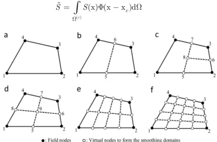
Figure 1: Division of quadrilateral element into smoothing domains in the cell-based smoothed finite element method: (a) nSC = _1;_(b)_nSC=_2;_(c)_nSC= _{3; (d)}_nSC= _{4; (e)}_nSC= _{8; (f)}_nSC= _16.

Figure 2: Design domain of the cantilever beam.

where F is the smoothing function written as:

( ) ( )

( )

1 / x (x x )

0 x

c c

A

ìï _{Î W}

ïï F - = í_ï

Ï W

ïïî (2.2)

where

( )

d

c

c A

W

=

_ò

W is the area of smoothing cell _W( )c _{. The element area is the sum of element cell}

areas:

( ) nSC

e c

c

(4)

Latin American Journal of Solids and Structures 13 (2016) 378-390 where nSC is the number of cells for each element. Note that this kind of smoothing is also employed

in the smoothed particle hydrodynamics method (Monaghan (1992)). Substituting F into Eq. (2.1), the smoothing strain can be written as:

( )

( ) ( )

1

n (x)u(x)d (x )d

c _n

c

u uI c I

c

I N

S

A _G Î

=

_ò

G =

å

 B

(2.4)

where _G( )c _{is the boundary of the smoothing cell}_W( )c _, n

N is the number of nodes per element,

(x )

uI c 

B is smoothing strain matrix of the domain _W( )c _{, and}_n( )c

u is the normal outward vector on the

boundary _G( )c _{. The vectors of} _{(x )} uI c 

B _and_n( )c

u are obtained as:

( ) x

( ) ( )

x

0

n 0

c

c c

u y

c c

y n

n

n n

é ù

ê ú

= ê ú

ê ú

ë û

(2.5)

(5)

Latin American Journal of Solids and Structures 13 (2016) 378-390 ( ) ( ) ( ) ( ) ( ) x ( ) ( )

d 0

(x ) (x ) 0

1 1

(x ) 0 d 0

d d

c b c b c c b b I x

g c g

I b b

uI c _c I y _c

I y I x

N n

N n

N n

A A

N n N n

G

G G

é ù

ê ú

ê G ú

ê ú

= _ê G _ú =

ê ú

ê G G ú

ê ú ê ú ë û

ò



B ( ) ( )

1 _{( )} _{( )}

x

(x ) (x ) (x ) (x ) (x ) (x ) nb

c g c g I b y b b

b g c g g c g

I b y b I b b

N n l

N n N n

= é ù ê ú ê ú ê ú ê ú ê ú ë û

å

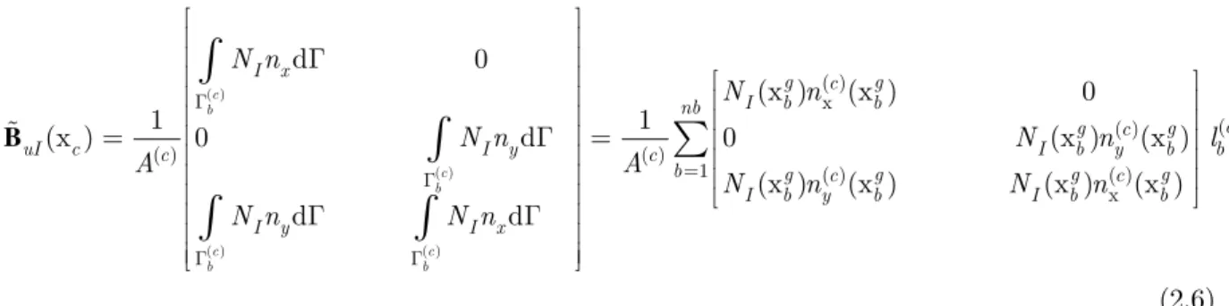
(2.6)

In the above equations, nb is the total number of boundary sections of ( )c b G , xg

b is the midpoint

(Gauss point) of the each smoothing domain boundary segment ( )c b

G , and ( )c b

l is the length of each

segment of ( )c b

G . It can be pointed out from Eq. (2.6) that unlike the finite element method, there is no derivative of shape function in the smoothing strain matrix. By employing the current formulation of the smoothed finite element method, the discrete equation for the cell-based smoothed finite ele-ment method is given as:

CS-FEM ₌

 

K U f (2.7)

where U is the vector of nodal displacements, f is the vector of nodal forces, and KCS-FEM is the

global smoothed stiffness matrix:

Figure 4: Evolution histories of the objective function over iterations, example 1.

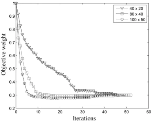
Figure 5: Evolution histories of the objective weight over iterations, example 1.

CS-FEM ₍ ( ) T₎ ( ) ( )

nSC

c c c

e u u

c

A

K =

å

B DB _(2.8)

(6)

Latin American Journal of Solids and Structures 13 (2016) 378-390

3 FORMULATION OF TOPOLOGY OPTIMIZATION PROBLEM

3.1 Optimization Problem

The objective of topology optimization is the optimal distribution of material in the design domain to minimize the cost functionals under various constraints such as stress, displacement or weight constraints. In this study, the aim is to find the stiffest structure subject to a given structural weight. Therefore, the optimization problem can be formulated as:

CS-FEM T CS-FEM

1

Minimize ( )=

Subject to : ( )=

: 0 or 1 =1,...,

e

N

e e e e e

req

e e

C x

W W

x e N

T

x U K U = u K u

x = = "

å

    (3.1)

where C( )x is the structural compliance, _W_{( )}x is the weight of the current topology,

req

W is the

prescribed weight and =( ,...,₁ )

e

N

x x

x is the vector of element densities. The design variable

e

x

indi-cates the presence (1) or absence (0) of an element, where e is the element index. u_e is the element

displacement vector and CS-FEM e

K _{is the element stiffness matrix for element}_e_{. In this study, the}

discrete level set method is employed to find the solution for the optimization problem. The discretized level set function y can be defined as:

( ) 0 if 1, ( ) 0 if 0.

e e e e x x y y c c

ìï < =

ïí

ï > =

ïî (3.2)

where c_e is the center position of element _e. Here,  is initialized as a signed distance function and

an upwind finite difference scheme is employed to accurately solve the evolution equation. The dis-crete level set function is updated to find new structure using the following equation:

(7)

g t

y _u _y _w

¶ _{= - }

-¶ (3.3)

where t indicates time, u is scalar field on the design domain, w is a positive parameter that specifies the influence of g, and g is a forcing term that determines the nucleation of new holes within the structure. Note that to satisfy the weight constraint, two parameters u and g are obtained based on the shape and topological sensitivities of the Lagrangian framework.

4 NUMERICAL EXAMPLES

In this section, three widely studied examples in the field of topology optimization are presented to show the effectiveness of the proposed method. Poisson’s ratio m = 0.3 and Young’s modulus of

1

E = are used for all examples.

4.1 Example 1

Fig. 2 shows the design domain of a cantilever beam with a length to height ratio of 2:1. The objective function is to minimize the compliance and the objective weight is 45% of the total weight of the design domain.

Figure 7: Design domain of beam with fixed support.

Figure 8:Evolution histories of the objective function over iterations, example 2.

(8)

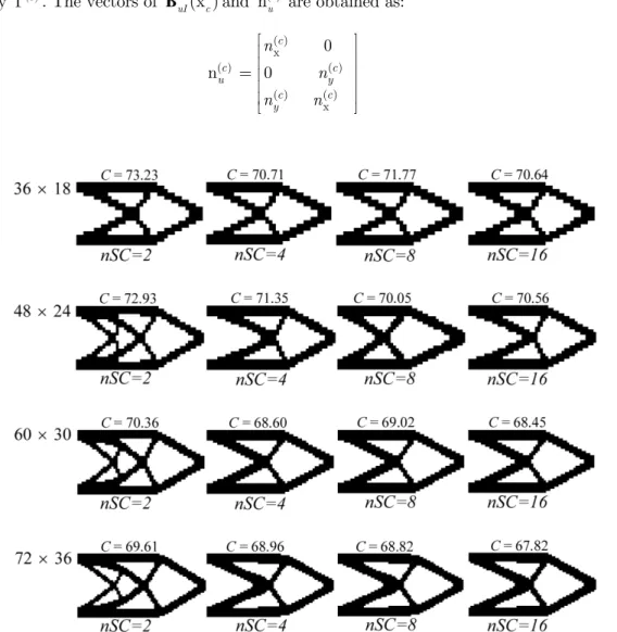
Latin American Journal of Solids and Structures 13 (2016) 378-390 To determine the optimal structural layout, the design domain is discretized using 36



18, 48



24, 60



30 and 72



36 quadrilateral elements. And to study the effects of the number of the smoothing cells, each element is subdivided into different number of smoothing cells using nSC =2,nSC = 4,

8

nSC = and nSC =16. The optimization results obtained from different mesh sizes with different

number of smoothing cells are shown in Fig. 3, from which it can be seen that the final solutions obtained from nSC = 4, nSC = 8 and nSC =16 with different mesh sizes are almost identical,

and are different from those obtained from nSC =2. The optimization results obtained using 2

nSC = show the so-called mesh dependency effect, for which different optimal topologies are

gen-erated from different mesh sizes. It can be found that the use of four (nSC =4) or more than four

smoothing domains can be good choices for topology optimization problems to overcome numerical instabilities such as mesh dependency phenomenon.

Figs. 4 and 5 illustrate the history of objective function and objective weight using nSC =4

based on different mesh sizes over iterations, respectively. It can be seen from Figs. 4 and 5 that the number of iterations for mesh sizes of 36



18, 48



24, 60



30 and 72



36 are 65, 57, 53 and 47, tively and their corresponding compliances are calculated as 70.71, 71.35, 68.60 and 68.96, respec-tively. It can be also seen from these results that for different mesh sizes, their convergence charac-teristics are very similar.

Figure 10: Results obtained by the present method with different mesh discretizations.

To verify the present method, the above problem using the same mesh sizes is solved by the Solid Isotropic Microstructure with Penalization (SIMP) method (Sigmund (2001)) (standard finite ele-ment-based method). The optimal structural layouts without and with sensitivity filtering are shown in Fig. 6, from which it can be seen that with and without using a filter, the topologies obtained from the SIMP method are quite different. Note that the SIMP method using a filter generates similar topologies to the designs obtained by the present method using nSC = 4, nSC = 8 and nSC =16

(9)

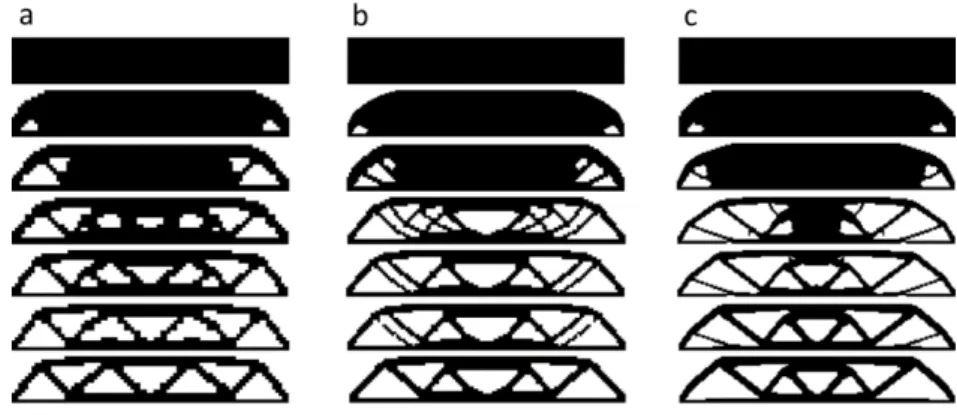
Figure 11:Evolution of topology at various mesh discretizations: (a) 4020; (b) 8040; (c) 10050.

4.2 Example 2

Fig. 7 shows the design domain of a beam with fixed supports. The beam length to height size ratio is 2:1. The objective function is to minimize the compliance, and the target weight is 30% of the total weight of the design domain. The division of the element into four smoothing domains (nSC = 4) is

used as default in this example.

Figure 12: Results obtained by the SIMP method from different mesh sizes without and with sensitivity filtering.

(10)

Latin American Journal of Solids and Structures 13 (2016) 378-390 In order to show that the optimum structural layout is mesh independent and checkerboard free, the design domain is discretized using 40



20, 80



40 and 100



50 quadrilateral elements. Fig. 8 shows the evolution history of the objective function over iterations based on different mesh sizes. It can be observed from Fig. 8 that the number of iterations for mesh sizes of 40



20, 80



40 and 100



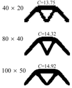
50 are 50, 53 and 46, respectively and their corresponding compliances are calculated as 13.75, 14.32 and 14.92, respectively. Fig. 9 shows the curves of convergence of the objective weight based on different mesh sizes. The almost monotonic and uniform convergence can be seen from this figure.

The optimization results obtained by the present method are shown in Fig. 10, the topology optimization history at various iterations is shown in Fig. 11, and the optimization results obtained by the Solid Isotropic Microstructure with Penalization (SIMP) method (Sigmund (2001)) (standard finite element-based method) without and with sensitivity filtering are shown in Fig. 12. From these results it can be seen that the SIMP method using a filter produces similar topologies to the present method, and the present method can effectively remove numerical instabilities such checkerboard pattern and mesh dependency phenomena. The number of iterations of the SIMP method for mesh sizes of 40



20, 80



40 and 100



50 are 41, 96 and 123 respectively and their corresponding compli-ances are respectively calculated as 15.14, 15.12 and 14.53. It is confirmed that the number of itera-tions of the present method is less than the SIMP method, and a smoother optimization result can be obtained by the present method.

4.3 Example 3

The design domain of a simply supported Michelle type structure with a length to height ratio of 6:1 is shown in Fig. 13. The objective function of this example is to minimize the compliance and the objective weight is 50% of the total weight of the design domain.

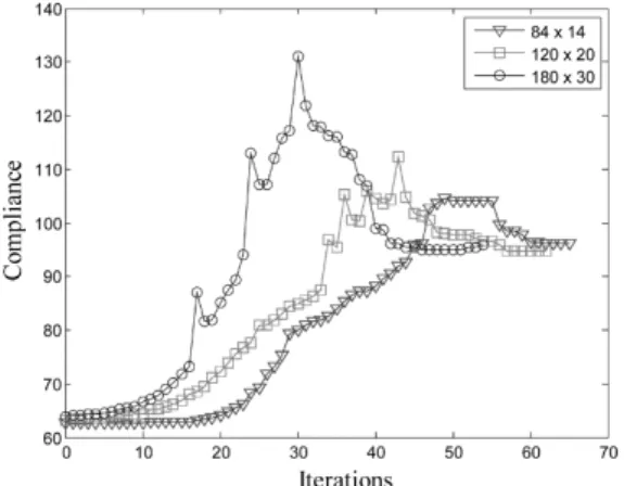
Figure 14:Evolution histories of the objective function over iterations, example 3.

(11)

Figure 16:Results obtained by the present method with different mesh discretizations.

In order to show that the solution is mesh independent and checkerboard free, the design domain is discretized using 84



14, 120



20 and 180



30 quadrilateral elements. Each element is subdivided into four smoothing domains (nSC =4). Fig. 14 shows the evolution history of the objective function

over iterations, and Fig. 15 gives the curves of convergence of the objective weight based on different mesh sizes. The number of iterations for mesh sizes of 84



14, 120



20 and 180



30 are 65, 63 and 55, respectively and their corresponding compliances are calculated as 96.15, 94.82 and 95.82, respectively. It should be noted that the occasional jumps in Fig. 14 may be attributed to a remarkable alteration of topology due to the elimination of one or more bars in a single iteration.

The optimum structural layouts and the topology optimization history at various mesh sizes are shown in Figs. 16 and 17, respectively. The optimization results obtained by the Solid Isotropic Microstructure with Penalization (SIMP) method (Sigmund (2001)) (standard finite element-based method) are given in Fig. 18. A comparison between the final solutions shown in Figs. 16 and 18 shows that the two different optimization methods generate similar topologies and the present method can avoid numerical instabilities such as checkerboard pattern and mesh dependency phenomena. The compliances of the solutions of the SIMP method for mesh sizes of 84



14, 120



20 and 180



30 are respectively calculated as 101.92, 103.81 and 100.22 which are higher than those of the present method. These differences may be due to the over-estimated strain energy of elements in the solutions of the SIMP method.

(12)

Latin American Journal of Solids and Structures 13 (2016) 378-390 Figure 18:Results obtained by the SIMP method from different mesh sizes without and with sensitivity filtering.

4 CONCLUSIONS

In this paper, the smoothed finite element method is combined with the level set method to develop an efficient approach for topology optimization of continuum structures. The cell-based smoothed finite element method is employed to improve the accuracy and stability of the standard finite element method. Several numerical examples were presented to show the validity and feasibility of the pro-posed method. The examples have shown the effectiveness of the propro-posed method to overcome nu-merical instabilities such as checkerboard patterns and mesh dependency phenomena. As a future research work, the proposed approach can be efficiently used to solve structural topology optimization problems with other objective functionals and constraints such as stress or displacement constraints.

References

Amstutz, S., Novotny, A.A., de Souza Neto, E.A., (2012). Topological derivative-based topology optimization of struc-tures subject to Drucker–Prager stress constraints. Computer Methods in Applied Mechanics and Engineering 233-236:123-136.

Atluri, S.N., Zhu, T., (1998). A new meshless local Petrov-Galerkin (MLPG) approach in computational mechanics. Computational Mechanics 22:117-27.

Belytschko, T., Lu, Y.Y., Gu, L., (1994). Element-free Galerkin method. International Journal for Numerical Methods in Engineering 37:229-256.

Bendsøe, M.P., Sigmund, O., (2003). Topology Optimization: Theory, Methods, and Applications. Springer, New York, USA.

Burger, M., Hackl, B., Ring, W., (2004). Incorporating topological derivatives into level set methods. Computational Physics 194:344-362.

Dijk, N.P., Maute, K., Langelaar, M., Keulen, F.V., (2013). Level-set methods for structural topology optimization: a review. Structural and Multidisciplinary Optimization 48(3):1-36.

Hassani, B., Hinton, E., (1999). Homogenization and Structural Topology Optimization: Theory, Practice and Soft-ware. Springer, New York, USA.

(13)

Liu, G.R., Dai, K.Y., Nguyen, T.T., (2007). A smoothed finite element method for mechanics problems. Computational Mechanics 39:859-877.

Liu, W.K., Jun, S., Li, S., (1995). Reproducing kernel particle methods for structural dynamics. International Journal for Numerical Methods in Engineering 38(10):1655-79.

Lopes, C.G., dos Santos, R.B., Novotny, A.A., (2015). Topological derivative-based topology optimization of structures subject to multiple load-cases. Latin American Journal of Solids and Structures 12(5):834-860.

Luong-Van, H., Nguyen, T.T., Liu, G.R., Phung-Van, P., (2014). A cell-based smoothed finite element method using three-node shear-locking free Mindlin plate element (CS-FEM-MIN3) for dynamic response of laminated composite plates on viscoelastic foundation. Engineering Analysis with Boundary Elements 42:8-19.

Monaghan, J.J., (1992). Smoothed particle hydrodynamics. Annual Review of Astronomy and Astrophysics 30:543-574.

Nguyen, T.T., Liu, G.R., Lam, K.Y., Zhang, G.Y., (2009). A face-based smoothed finite element method (FS-FEM) for 3D linear and geometrically non-linear solid mechanics problems using 4-node tetrahedral elements. International Journal for Numerical Methods in Engineering 78:324-353.

Nguyen-Thanh, N., Rabczuk, T., Nguyen-Xuan, H., Bordas, S., (2008). A smoothed finite element method for shell analysis. Computer Methods in Applied Mechanics and Engineering 198(2):165-177.

Nguyen-Xuan, H., Rabczuk, T., Bordas, S., Debongnie, J.F., (2008). A smoothed finite element method for plate analysis. Computer Methods in Applied Mechanics and Engineering 197(13):1184-1203.

Shobeiri, V., (2015a). Topology optimization using bi-directional evolutionary structural optimization based on the element-free Galerkin method. Engineering Optimization. doi: 10.1080/0305215X.2015.1012076.

Shobeiri, V., (2015b). The topology optimization design for cracked structures. Engineering Analysis with Boundary Elements 58:26-38.

Sigmund, O., (2001). A 99 line topology optimization code written in MATLAB. Structural and Multidisciplinary Optimization 21(2):120-127.

Xie, Y.M., Huang, X., (2010). Evolutionary Topology Optimization of Continuum Structures: Methods and Applica-tions. John Wiley & Sons, New York.