Page 1 of 1
Lancaster University
Department of
Accounting and Finance
AcF 706 – CFA-Stream
Dissertation
August 2013
Xinqi Cheng
This dissertation is submitted in partial
fulfilment of the degree of MSc in Finance
I
Accessing Default Risk of a Public
Company with Structural Models
AcF 706 – CFA-Stream Dissertation Accessing Default Risk of a Public Company
Lancaster University Management School
Xinqi Cheng
Abstract
There are various ways to evaluate the credit risk of a public company using both market data as well as accounting data. This paper focuses on applying two structural models, Merton (1974) and Leland (1994), to access the default risk of a public company, Thomas Cook Group plc. With estimated default probabilities higher than 90% during 2011 to 2012, it is shown that both models can predict bankruptcy, which is in the form of debt restructuring and capital refinancing in early 2013. The Leland model also suggests that there exists an optimal capital structure that could minimize the credit spread.
Key words: default probability, credit spread, structural model, public firm.
II
Table of Content
1. Introduction ... 1
2 Literature Review... 2
2.1 Credit Risk and Credit Spread ... 2
2.2 The Evolution of the Structural Models ... 5
2.3 Empirical Evidence ... 8
2.4 Other Bankruptcy Prediction Models ... 11
2.4.1 The Accounting Information Based Models ... 11
2.4.2 Other Models of Credit Risk Measurement ... 12
3. Data and Sample Selection: Thomas Cook Group plc ... 13
3.1 Descriptive Analysis ... 13
3.2 Financial Analysis ... 14
3.3 Share Price Analysis... 16
3.4 Altman Z-scores ... 18
4. Calibration of the Models ... 19
4.1 Methodology ... 19
4.1.1 Merton Model ... 20
4.1.2 Leland Model ... 22
4.2. Sensitivity Analysis ... 23
4.2.1 Hypothesis and Methodology ... 23
4.2.2 Results ... 24
4.3 Empirical findings ... 29
4.4 Comparative analysis ... 31
5. Conclusion ... 34
III
List of Figures
Figure 1: Relative Stock Price of TCG, the FTSE ALL Share and the FTSE 250 ... 16
Figure 2: Market Value of TCG ... 17
Figure 3: Volatility against Credit Spread in the Merton Model ... 25
Figure 4: Volatility against Credit Spread in the Leland Model ... 25
Figure 5: Leverage against Credit Spread in the Merton Model ... 26
Figure 6: Leverage against Credit Spread in the Leland Model ... 26
Figure 7: Risk-free Rate against Credit Spread in the Merton Model ... 28
Figure 8: Risk-free Rate against Credit Spread in the Leland Model ... 28
Figure 9: The Default Probabilities of the Models ... 32
Figure 10: The Credit Spreads of the Models ... 32
Figure 11: The Estimated Debt Values and the Market Value of Bonds ... 33
List of Tables Table 1: Financial Analysis ... 15
Table 2: Altman Z-score ... 18
Table 3: Acronyms ... 19
Table 4: Selected Variables and Hypothesis ... 23
Table 5: Sensitivity Analysis ... 24
Table 6: Merton Model ... 29
1
1. Introduction
The value of a firm could have considerably significant impact on its credit risk. In a simplified corporate capital structure, the firm asset is normally contributed by equity and liabilities, while the returns to each of the components can be decomposed into risk-free rate of return and risk premium. Defined as the difference between the yield of corporate bond and that of treasury-bill which is considered “risk-free”, the yield spread of a straight (option-free) bond is determined by liquidity risk, credit risk and interest rate risk. Thus a change in credit risk would alter the cost of debt, and thereby affect the cost of capital and capital structure for the future.
In the event of default, the company fails to meet the either the coupon or principal repayments of the obligations, and then the process of bankruptcy is triggered, meaning that the investors could only gain back a portion of their initial investments. Worse still, creditors may be required to pay the salaries and other service fees to the lawyers and accountants before they could claim the remaining asset of the firm. Hence, even though companies that actually bankrupt are of a relative small portion in the real corporate world, bond investors are concerned about credit risk and default probability.
Currently there are numerous ways to measure the enterprise credit risk, including qualitative assessment tools such as the concept of 5 Cs (Capacity, Capital, Conditions, Character and Collateral), and quantitative tools which measure the likelihood of default and price default risks, such as the reduced-form approach, which uses intensity-based models to estimate stochastic hazard rates. Also, standing somewhat in between, are rating agency grades, which usually are judgemental assessments of both qualitative and quantitative factors.
For decades academics have been trying to measure and price credit risk by constructing structural models, among which Merton (1974) is the most widely applied and studied. By modelling the stochastic evolution of the firm value, structural models value the default risk and price the corporate debt. Based on the Black-Scholes option-pricing formula, Merton (1974) prices the equity as though it were a call option with the strike price which is the book value of the liabilities. The Merton model is a milestone in the development of such models, and since then
2
various models have been constructed by resolving the naive assumptions of the Merton model and by adding additional boundary conditions.
Assuming that default is triggered at the first time at which the firm value falls below a certain threshold which need not be the book value of debt, Leland (1994) shows how such threshold could be determined. Incorporating tax benefit and bankruptcy cost of debt, Leland assumes that bankruptcy could be a policy to maximize the value of equity. Extending the idea of Leland (1994), Mella-Barral and Perraudin (1997) shows debt renegotiations could eliminate agency cost and bankruptcy cost, which is beneficial to several parties of stakeholders. It is suggested that the structural models could favour the financial decision making process.
By performing a detail analysis of a chosen firm using the Merton model and the Leland model, this paper compares the results and reconciles the differences to examine the validity and accuracy of these two models in forecasting bankruptcy. The empirical findings show that both models display consistent results of the default probability and credit spread of the firm. In a further sensitivity analysis of some of the variables of the models, it is found that under the structure of Leland model, there is an optimal capital structure that could minimize the credit spread if maintaining the price value.
The paper is structured as follow. Section 2 reviews the literature of credit risk, major bankruptcy prediction models and their empirical evidences. Section 3 is a financial analysis of the target firm, Thomas Cook Group plc, using accounting data as well as market data. Section 4 displays the implementation of Merton model and Leland model to the target firm and the analytical results, including a sensitivity test. Section 5 concludes.
2 Literature Review
2.1 Credit Risk and Credit Spread
A company defaults when it fails to meet its obligations. The probability of default is then described as credit risk. Bai et al. (2011) summarize the characteristics of credit risks as non-symmetry, cyclicality, non-systematic and infectiousness. Since structural models are to predict probability of default, inputs of such models may
3
provide knowledge about the determinants of credit spread. On the other hand, identifying the sources and drivers of default risk could help better evaluate the performance of these models.
Traditionally the sources of risk could be categorised as systematic and non-systematic, that is, the credit risk determinants could be divided into macroeconomic and firm-specific factors. Bonfim (2008) argues that firm-specific factors could provide better assessment of credit risk when macroeconomic factors were taken into account, which is in line with Tang and Yan (2010), who also concluded that the most important credit risk determinant at the firm level is implied volatility and that at the market level is investor sentiment.
It is documented that default probabilities vary in different stages of business cycle, i.e. credit spread is counter-cyclical. Tang and Yan (2010) hypothesize that credit spreads widen during recessions and narrow during economic expansions. They also argue that the investor sentiment is a dominant source of credit risk at the market level. With some statistical analysis, Yamachi (2003) finds that the market price of risk is high at times of high risk, concluding that the risk tolerance of investors had an impact onto the credit spreads. This is consistent with the idea that during recessions investors are more risk-averse and thus ask for higher compensation for bearing credit risk.
Elton et al. (2001) try to explain why a risk premium exists in corporate bonds and conclude that the major portion of the difference is the compensation for bearing systematic risk, implying that the Fama-French (FF) factors, SMB1 and HML2, would influence the credit risk. This is in line with Vassalou and Xing (2004) that study the effect of default risk on equity returns, concluding that default risk is systematic and is priced into the excess stock return. Indeed, Fama and French (1996) argued that SMB and HML are financial distress related proxies. Adding an aggregated survival measure into the regression model of excess stock return against excess market return, Vassalou and Xing (2004) show that SMB and HML share common information with
1
SMB stands for “Small minus Big”, which is the yield spread between small-capitalization companies and large-capitalization companies.
4
survivorship, but SMB has little pricing power. Interestingly, Schaefer and Strebulaev (2008) also include the FF factors in their examination of credit spread variables and find that the corporate bond returns are considerably sensitive to SMB. Despite the previous empirical evidence, how such systematic factors play a role in the determination of credit spreads remains unclear.
Contrary to the findings of Elton et al. (2001), using the cross-sectional data on corporate yield spreads, King and Khang (2000) find that the bond sensitiveness to the equity market provides very limited explanatory power once the default-related factors are controlled for. One reason for this controversy is that the different choices of proxy are not empirically justified and thus may yield different results. Huang and Huang (2003) question the rationale of Elton et al. (2001), in that the expected default loss does not substantially represent credit spread. The expected default loss rate may be systematic, while credit risk premium, which is also a component of credit spread, is subjected to firm-specific information.
Most of the firm-specific factors for credit risk, however, are intuitively indicated in the structural models. So far the most comprehensive research of the determinants of credit spreads is Collin-Dufresne et al. (2001). Overall they find these variables of statistical and economic significance but little explanatory power to the credit spread changes. The possible determinants and their intuition are as follows:
1. The level of risk-free rate is negatively related to credit spread, consistent with the empirical findings of Longstaff and Schwartz (1995). Collin-Dufresne et al. (2001) also find that the sensitivity of risk-free rate increases as the firm moves towards bankruptcy.
2. The term structure of yield curve is also negatively related to credit spread. Since an upward-sloping term structure implies higher future spot rates, the negative relationship is reasonable given the previous argument. Moreover, the downward-sloping term structure may imply economic recession, during which the credit spread would increase. However Collin-Dufresne et al. (2001) find its influence of economic significance.
3. Implied volatility is positively associated with the credit risk. As the structural models model the securities as options, higher stock market volatility would lead to larger credit spreads, and implies higher risk-aversion and default
5
probability (Yamachi 2003). In a further univariate regression analysis Collin-Dufresne et al. (2001) find that a given increase in volatility would affect the credit spreads more proportionately than an equal decrease.
4. Leverage is positively related to credit spread. Furthermore, higher leverage ratios would decrease return on equity, which could also widen the credit spreads.
5. Expected downward jumps in the firm value and the credit spread have a positive relationship. This is motivated by the volatility smiles in the observed option prices, which the Black-Scholes option pricing formula fails to capture. Collin-Dufresne et al. (2001) find that with increasing market expectation of negative jumps, the credit spreads would expand.
6. The expected recovery rate is negatively associated with the default probability. The recovery rates are indicators for the overall economic conditions and business climate. Taking the S&P 500 returns as proxy, both Collin-Dufresne et al. (2001) and Schaefer and Strebulaev (2008) find it statistically and economically significant.
In addition to the determinants tested in Collin-Dufresne et al. (2001), Schaefer and Strebulaev (2008) and Yamachi (2003), studies suggest there are missing firm-specific factors that affect the credit spreads. Ogden (1987) and Vassalou and Xing (2004) suggest the size effect is an additional default-related variable. Corporate and personal taxes may also influence the credit spread in that the firms may or may not fully exploit the tax benefit (Lyden and Saraniti 2001; Qi et al. 2011). Yamachi (2003) quotes Schmid (2002) that liquidity may be a determinant but find little supportive evidence.
2.2 The Evolution of the Structural Models
There has been much literature trying to value securities without an active trading market or public available information to obtain the directly observable price. Merton (1974) is the very first model to “structure” the firm value and the economic process leading to default. Briefly, in a risk-neutral world, the Merton model uses the Black-Scholes option pricing formula to price the equity of the firm as a call option which could be exercised at the book value of liabilities, and describe the dynamics of firm value as a stochastic process. The value of corporate debt is calculated as the firm
6
value deducted by the previous call option. Alternatively, the liabilities could be viewed as the short position of a put option plus safe assets. A detailed methodology of the Merton model is discussed in section 4.1.1.
On pricing the corporate debt, Merton (1974) assumes that: a) the market is perfect and frictionless; b) assets are traded continuously in time; c) the Modigliani-Miller theorem holds; d) the yield curve is flat; and e) the firm asset returns follow a geometric Brownian motion. Based upon these assumptions, the Merton model could be used to price single-issued, zero-coupon risky debt, on the condition that there is no dilute payment prior to maturity. Upon maturity, once the asset value falls below the book value of debt, default is triggered, resulting in bondholders taking control of the firm and equity holders receiving nothing.
As the assumptions of Merton (1974) are naive and restrictive compared to what are observed in reality, scholars raise newer models to resolve these assumptions, and bring modifications and complications to varied situations. Geske (1977), for instance, adjusts the Merton model to multiple maturity dates and modifies the boundary conditions to asset dilution, i.e. either debt or equity refinancing.
A flow of literature is to relieve the assumptions that default can only occur on maturity date, i.e. default could occur prior to maturity. Also, the assumption of perfect anti-dilution is resolved, that is, coupon payments could be refinanced by issuing equity.
Black and Cox (1976) is an instance, introducing the idea that default would occur if the firm value falls below a pre-specified level, rather than after the firm assets have been exhausted. Since such bond indentures as net-worth covenants, subordination agreements and restrictions on dividend payments could be served as a time-dependent default boundary, the claims on assets may behave differently and then the securities are priced accordingly.
Following Black and Cox (1976), Leland (1994) argues that bankruptcy is determined endogenously and thereby alters the bankruptcy-triggering conditions of the firm and time horizon of the bonds in his model. Assuming that the corporate bonds have infinite life and constant coupon payment, the Leland model includes the tax shield value and bankruptcy cost into the total value of the firm and shows how the default
7
threshold could be determined in such setting. Detail application of the Leland model is discussed in section 4.1.2.
The structural models then become an integral part of corporate finance and corporate governance. Leland and Toft (1996) show how the bankruptcy could be determined and severed as the optimal decision made in the benefit of equity holders, assuming that the firm can actively choose the amount and maturity of debt. Contrary to Lonstaff and Schwartz (1995), the model presumes a non-stochastic process for interest rate to simplify the model, and relates the bond values to a group of variables, namely, firm value, asset volatility, leverage, bankruptcy cost, tax rate, payout ratio as well as default-free interest rate.
As documented in empirical evidences, there is a certain portion of risk premia in the event of bankruptcy settlement observed in the actual security market that could not be captured by the Merton model. Leland and Toft (1996) also point out that long-term debt could take advantage of a tax shield, but may raise the problem of agency cost of debt and asset substitution. Arguing that such high default premia in junior claims is caused by strategic persuasion and bargaining of equity holders to bondholders, Mella-Barral and Perraudin (1997) propose formulae to value equity and debt with the assumptions that there is no tax advantage to debt and the debt is perpetual. The Mella-Barral and Perraudin model shows how the bankruptcy cost and agency cost of debt could be reduced or eliminated by the renegotiation of debt between the two counterparties.
Suggested by Jones et al. (1984) and Ogden (1987) that stochastic interest rates could help improve the predictive accuracy, the Merton model is extended to two-factor models. Resolving the assumptions of constant interest rate and simple bond issue, Longstaff and Schwartz (1995) extend Black and Cox (1976) to a two-factor model with non-flat credit spreads. By incorporating both default risk and interest rate risk, this model allows for the firm assets being correlated with the interest rates and the default-free interest rates following a stochastic process. Taking a step forward, with the evidence that companies may rebalance the debt levels in response to changes of firm value so as to target some favourable capital structure, Collin-Dufresne and Goldstein (2001) propose a model with stochastic interest rates that captures the mean-reversion of leverage ratios. They show that the model is more consistent with
8
the empirical observation that the leverage ratio of the firm is stationary and that the yield curve of speculative corporate bonds is upward-sloping.
2.3 Empirical Evidence
Without empirical tests, choosing the most applicable models may remain a difficult task. However less effort has been made so far to empirically examine the structural models comparing to that of constructing theoretical foundations. This part of literature review will focus on three questions:
1. How informative are these structural models?
2. To what extent can each structural model explain the variation of credit spreads?
3. Are the models robust, i.e. are there any inputs missing in these models? Although the results of empirical tests are conflicting, generally the studies show that these structural models can provide considerable amount of information for credit rating and the variations in credit risk. In a simple sign test of default presented in Jones et al. (1984), the contingent claims model significantly outperform the naive accounting-based model.
Delainedis and Geske (2003) find that both Merton model and Geske model do well in forecasting credit migration. They calculate series of monthly risk-neutral default probability (RNDP) with the two models for the period of 1988 to 1999 and then examine the variation of these default probabilities prior to default or credit migration on both ex-post and ex-ante bases. At the event window, the difference between the median RNDP of the selected companies (“raw”) and that of the control group (“base”) is noticeable for a given time period before credit migration.
The even more significant difference for non-investment grade bonds indicates that the structural models may work better for junk bonds, which is in line with Jones et al (1984), that the Merton model does provide incremental explanatory power for pricing riskier debts. Huang and Huang (2003) have similar conclusion that credit risk could explain a larger proportion of yield spread for junk bonds. To be more specific, Delainedis and Geske (2003) present that, with the Merton model for example, for the investment grade bonds, 17 months prior to bonds being re-rated, such difference is significant at both the 95% and 99% level. Among the investment grade bonds, the
9
event that possesses least detectable information is that the firm experience more than 2 rating categories upgrading. The raw RNDP for non-investment grade bonds, 24 months and 1 month prior to the event, are 14% and 62.4% respectively, which are significant. Even for the non-investment grade bonds with no previous history of downgrading, it transpires that the 99% significance level arrives at 18 months prior to credit migration.
Ogden (1987) also finds evidence that such inputs as asset volatility and leverage could explain 78.6% of the variation of agency bond ratings and could also correctly classify 61.4% bonds into the corresponding ratings. The sample contains 57 callable and sinkable corporate bonds of the firms with simple capital structure, from 1973 to 1985. With the sample data, Ogden (1987) shows that the modelled yield spread could explain approximately 60% of the observed market yield spread.
The answers for the second question, however, are mixed. Jones et al. (1984, 1985) are the very first studies of the empirical validity of the Merton models. Jones et al. (1985) question the assumptions of the model and confirm the effects of personal tax, time-varying variance and asset dilution on pricing debts. They compute the monthly bond prices for 15 firms with the characteristics of simple capital structure, small portion of private and short-term debt from 1975 to 1981, and point out that the Merton model underprices the “safe” bonds with maturity shorter than 15 years but overprices the bonds with otherwise similar characters. Nevertheless, Fisher (1985) comments that the contingent claims model is originally constructed to price risky bonds not “safe” bonds and questions the methodology in Jones et al. (1985) that the variance might be correlated over time as they take the history volatility as the future implied volatility.
With the growing body of literature in constructing various structural models, some studies focus on comparing the extent of accuracy to which the models are able to price risky bonds. Eom et al. (2004) examine 182 bond prices from non-financial firm in the period of 1986 till 1997 and concluded that the Merton model predicts too low credit spreads while other models, namely, Geske (1977), Longstaff and Schwartz (1995), Leland and Toft (1996), Collin-Dufersne and Goldstein (2001), overestimate the credit spreads.
10
Overall, the empirical results of the prediction accuracy are not satisfying. Schaefer and Strebulaev (2008) infer two possible reasons for the failure of the models. One would be the oversimplification of the long-term financial policies of the companies. The other is that the bond prices may be affected by non-credit issues that are not considered in the models. Such questioning about missing factors is also implied by the large and significant intercept in regression analysis of observed market yield spreads against the bond yield spreads (Ogden 1987).
This leads to the third question and answers to it are indeed what trigger the development and evolution of the structural models.
Both Jones et al. (1984) and Ogden (1987) suggest that the contingent claims models should incorporate some intuition of interest rates to replicate the risk-free bond prices and reflect the risk premium. Nonetheless, Lyden and Seraniti (2001) find proofs that the stochastic interest rate accounts for a very limited portion of the prediction accuracy. One possible explanation is that both Jones et al. (1984) and Ogden (1987) choose a period with high interest rate volatility and thus the interest rate variation may appear to be influential. Eom et al. (2004) shows that the problem of inaccuracy in the Lonstaff and Schwartz model, the Leland and Toft model and the Collin-Dufersne and Goldstein model is actually worsened by incorporating bankruptcy cost and stochastic interest rates.
Ogden (1987) proposes the firm size could be an additional input of the structural models. Once the firm size is added, when the default risk measures derived from the model are controlled for, the explanatory power to bond ratings variation raises to 85.5%.
Raised by Jones et al. (1984) and supported by Lyden and Seraniti (2001), personal tax and time-to-maturity could be the missing variables of the models. Qi et al (2010) construct a model and argue that the predictive accuracy could be enhanced by taking personal tax and liquidity factors into consideration of pricing debts. Regarding the maturity effect, Huang and Huang (2003) find also that the credit risk can explain a smaller fraction of credit spread for investment grade bonds with shorter maturities. To the contrary, by holding volatility and leverage constant, Eom et al. (2004) claim that maturity contains no extra information for estimating the spreads.
11
The results and conclusions of the empirical tests are mixed, largely due to differences in the selected period and the choices of proxy. Credit risk premium could explain yield spread to some extent, but the question is whether the chosen proxies are empirically verified. Missing factors may also account for the inaccuracy of the structural models.
2.4 Other Bankruptcy Prediction Models
2.4.1 The Accounting Information Based Models
Using accounting information and financial ratios to predict bankruptcy has long been extensively studied. Academics employ various statistical tools to explore and construct models to classify failed companies and non-failed companies.
By applying univariate regressions to study default probability and financial ratios the rationale of univariate models is to compare the statistically significant financial ratios and then specify a cut-off point of the two classes of firms. Adopting this idea, Beaver (1966) constructed a cash flow model to measure the default probability. Later Beaver (1968) found out that using the stock market price data could predict bankruptcy sooner.
Another statistical approach using accounting information is the multivariate model, in which several independent variables are combined. Altman (1968) employs multivariate discriminate analysis and proposes an index of five financial ratios, which is called the Z-score. Arguing that the previous studies are based on data from already bankrupted companies and thus overstated the accuracy, Ohlson (1980) employs the conditional logit model and proposes another model to compute the so-called O-score with another set of variables. These two models are so far the most popular ones in empirical studies. Generally these multivariate predictive models outperform the previous univariate models.
Critics question the methodology of the multivariate models, arguing that there is no theoretical foundation for way the models were constructed, which is, starting with large numbers of candidate variables and then scaling down to the considerably significant ones. Zmijewki (1984) argues that the extremely low percentage of bankrupted firms relative to active firms and the unavailability of data after the firm
12
bankrupts would be two questionable methodological issues in these models. The generalizability of the models is also a problem. Grice and Ingram (2001) test the generalizability of Altman‟s model and find it to be of less predictive power in forecasting bankruptcy when using recent data and for non-manufacturing companies. Comparing the usefulness of several bankruptcy models, Hillegeist et al. (2004) conclude that the Scholes-Merton Probability model derived from the Black-Scholes-Merton option-pricing model provided significantly (at the 1% level) more information about default probability than any of the accounting-based models. Wu et al. (2011) find similar conclusions when they include more bankruptcy prediction models in their study. Hillegeist et al. (2004) and Altman and Sauders (1998) point out several disadvantages of the accounting-based measures in comparison of structural models: a) the probability of bankruptcy is forward-looking while accounting information is measures of past performance; b) they fail to incorporate the asset volatility; and c) accounting information could only be obtained periodically while the structural models could be implemented at any point of time.
2.4.2 Other Models of Credit Risk Measurement
Whilst many empirical tests find it difficult to estimate the non-observable parameters of the firm value in the implementation of the structural-form models, the reduced-form models are another family of structural models that attempt to tackle this issue. Rather than conditioning default explicitly onto the value of firm and structuring the firm value as a stochastic process, the reduced-form models consider default as a rare event, which is modelled as Poisson process.
Generally speaking, the credit spread calculated from the reduced-form models overstated the credit risk and hence may not provide direct measure of default probability. However, in the region where there is an active bond-trading market, the reduced-form models are widely adopted, given that the reduced-form models are fundamentally market-based models.
Despite the fact that the reduced-form models require fewer parameters, the theoretical foundation of these models are questionable, in that the reduced-form models fail to show where the risk comes from. Unlike reduced-form models, the structural-form models are able to evolve based on economic reasoning. Secondly, the
13
time-varying parameters would cut the validity of the reduced-form models down to a relatively short time period. A third criticism of the reduced-form models is lacking of mathematical trackablity.
Different from the models mentioned above, the Gambler‟s ruin model is a structural model that applies a gambling hypothesis to the case of company, and calculates the distance to default relying on the information of cash flow. To be more specific, Wilcox (1971) treats the equity as initial stake and the cash flow as having either positive and negative states, and then investigates the probability of losing the initial stake after certain number of games. The distance to default presents the risk as a function of value and volatility, which is calculated as the sum of equity and cash flow, divided by the cash flow volatility.
The Wilcox‟s gambler‟s ruin model is little known and less studied, as it problematically presumes that the company is isolated from the financial market, and thus could only partly explain corporate failure and business risk.
Moreover, with the development of mathematical approach and computational science, more powerful statistical tools are employed in the prediction of company failure. The hybrid models are the ones that apply data mining techniques in the computation of probability of bankruptcy. There is extensive literature regarding the construction of hybrid models involving such techniques as decision trees, neutral networks, genetic algorithm, support vector machine and so forth. Most of the studies that empirically test the hybrid models show higher predictive power in hybrid models than in accounting-based models.
3. Data and Sample Selection: Thomas Cook Group plc
3.1 Descriptive Analysis
Thomas Cook Group plc (TCG) is a travel agency company which is created in 2007 after a merger of Thomas Cook AG and MyTravel and is a constituent of FTSE 250. Its products are divided into three categories, namely, pre-packaged holidays, travel-related financial service and independent travel. Its core strategy is to maximize the mainstream package holiday and to seek a leading position in the independent travel industry.
14
TCG mainly operates in six geographic segments, which are all within the area of Europe and North America. Thus, during the recent financial crisis, TCG has suffered from huge turmoil and large losses because people are less willing to spend on holidays and other leisure activities. The ongoing uncertainty of global economy negatively impacts the international tourism industry. This reveals the fact that the tourism and travel industry is rather cyclical.
During the post financial crisis period, TCG changes the management team from top and adopt a series of plans to reduce cost and enhance profitability. In the financial year 2011 (FY2011)3, TCG suffers huge goodwill impairment and asset write-downs. Also, TCG proposes a reconstruction plan for the UK segment, of which the expenditure contributes to the significant loss in the first quarter of FY2012. TCG then reduces net debt by selling some of the business and eases financial burden by renegotiations of maturity extension.
Before 2013, TCG has two bond issues, one is a 5-year 6.75%-coupon straight bond issued in 2010 with face value of €400 million4
and the other is a 7-year 7.75%-coupon bond that matures in 2017 with face value of £300 million. On the first half-year of FY2013, TCG announces capital refinancing, which includes £425 million equity injection, £175 million net debt reduction and other debt renegotiations. On May 2013, the company issue £441 unsecured senior notes to replace some of the old bonds.
3.2 Financial Analysis
Panel A of Table 1 is the DuPont financial analysis of TCG. The profitability measured by return on equity (ROE) is decreasing year by year. The profit margin drops 4.5% to -3.08% for 2011. This negative profit margin, together with the huge jumps in tax burden and interest burden because of such loss, results in a negative ROE of -45%. In 2012, resulting from further declined equity to asset ratio, ROE is surprisingly -135.73%, indicating that TCG is in serious financial distress.
3 The accounting reference date of TCG is 30 September of each calendar year. 4 The face value of €400 million is converted in to £335.1 million in this paper.
15
Table 1 Financial Analysis
Using 5-year historic data from financial statements and the financial market, these accounting ratios are selected and classified into different groups for different purpose. The data was from Thomson ONE banker.
*Profit margin = Earnings before tax and interest / Total sales Tax burden = Net income / Pre-tax income
Interest burden = Pre-tax income / Earnings before tax and interest Asset Turnover = Sales / Average total assets
Equity multiplier = Total asset / Total common equity Return on Equity = Net income / Average equity
**The units for net cash flow from operating activities (CFO), net cash flow from financing activities (CFF) and net cash flow from investing activities (CFI) are millions of GBP (£M) and that for free cash flow per share is one unit of GBP (£).
***EBIT is the earnings before interest and tax; and EBITDA is the earnings before interest, tax, depreciation and amortization.
Cash flow analysis is an essential part in risk management and credit analysis. In panel B, the decreasing figures of net cash flow from operating and investing activities, as well as the cash flow to sales ratios indicate that the cash collection
2012 2011 2010 2009 2008 Profit margin -3.76% -3.08% 1.49% 1.81% 1.67% Tax burden 120.21% 128.19% -6.75% 26.38% 87.48% Interest burden 136.41% 134.37% 29.14% 35.72% 37.57% Asset turnover 1.57 1.52 1.35 1.39 1.46 Equity multiplier 14.03 5.59 3.79 3.89 3.35 Return on equity -135.73% -45.02% -0.15% 0.92% 2.68% CFO (£M) 35.4 196.2 234.3 75.5 302.0 CFF (£M) 32.8 10.7 -139.5 -226.5 81.1 CFI (£M) -52.7 184.3 291.1 130 291.5 Free cash flow (£M) -94.2 -14.1 -21.5 -142.9 141.6 Free cash flow per share (£) -0.0689 -0.0813 0.0077 0.0101 0.0313 Cash flow to sales ratio 0.52 1.20 2.98 2.48 2.24 Quick ratio 0.28 0.28 0.29 0.30 0.45 Current ratio 0.43 0.44 0.43 0.40 0.55 EBITDA/Interest expense -1.52 -1.30 3.37 3.45 4.88 EBIT/Interest expense -2.75 -2.91 1.41 1.45 2.08 Long-term debt/Equity 2.90 0.90 0.59 0.22 0.32 Total debt/Equity 3.07 1.07 0.67 0.72 0.59 Price-earnings ratio 1.80 1.30 8.30 8.70 7.30 Price to book ratio 0.38 0.30 0.85 1.16 1.00 Price to sales ratio 0.02 0.04 0.17 0.21 0.23 Price to cash flow ratio 3.07 2.92 5.54 8.63 10.49
Panel A: DuPont analysis*
Panel B: Cash flow analysis**
Panel C: Solvency analysis***
16
ability of TCG is diminishing over the five-year period. The negative free cash flows since 2009 also imply that there is little distributable cash available to equity holders and debt holders.
In panel C, both the quick ratios and current ratios are well below 0.5, meaning that the liquidity of TCG is problematic. In addition, the negative interest coverage ratios5 in 2011 and 2012 imply that TCG might have to liquidize some of its assets to cover the interest payments. The leverage ratios suddenly jump in 2012, which is caused by the plumped equity value.
In penal D of Table 1 are some valuation ratios. All ratios change dramatically in 2011, a period when the stock price is at historically low level. The price-earnings ratio of 2009 is the highest but it is below 2 in the recent two years. These decreasing valuation ratios suggest that investors are passive towards the stock performance of TCG.
3.3 Share Price Analysis
Figure 1
Relative Stock Price of TCG, the FTSE All Share and the FTSE 250 Based on the stock price and price index values on 19 June 2007, which is the date when the merger between Thomas Cook AG and MyTravel completes, the relative prices are calculated and presented in percentage term in each dataset respectively. Data is extracted from Datastream and complied by author for the period from June 2007 to May 2013.
5 The interest coverage ratios are EBIT/Interest expense ratio and EBITDA/Interest expense ratio.
0% 20% 40% 60% 80% 100% 120% 140% 160% 19/06/2007 19/06/2008 19/06/2009 19/06/2010 19/06/2011 19/06/2012 Relat ive price FTSE 250 FTSE ALL TCG
17
Figure 2
Market Value of TCG
In 2007 after the merger of Thomas Cook AG and MyTravel, the market value of TCG inflates to over £3,000 million. The market value declines in the following period and is volatile at the level of £2,000 million. Then it falls sharply in 2011 and is below £250 million in 2012. Data is extracted from Datastream and complied by author for the period from January 2007 to May 2013.
Judging from Figure 1 and 2, though TCG initially outperforms the market, its volatility is considerably more significant than the FTSE All Share and the FTSE 250. Even though the stock price starts to bounce back at the beginning of 2013, its current relative stock price is still below the level of the FTSE.
Both the relative price level and market value start to drop significantly when Standard and Poor‟s (S&P) downgrades TCG to BB- with negative outlook, arguing that TCG might be unable to repay its debt upon maturity. With the speculation of worsening trading environment, S&P further lowers the long-term corporate rating to B on November 2011, causing the stock price drop to historical low level. On July 2012, TCG is rated B- but then is upgraded to B after the recapitalization in July 2013.6
TCG has announced dividend payments and share repurchases several times since 2007, but two of the dividend announcements are omitted, in December 2011 and
6 Source: Standard & Poor‟s Financial Services LLC (www.standardandpoors.com).
0 500 1000 1500 2000 2500 3000 3500 19/06/2007 19/06/2008 19/06/2009 19/06/2010 19/06/2011 19/06/2012 MV (£ M)
18
May 2012 respectively, which signals financial distress of TCG. TCG decides not to pay any dividend until the organizational restructuring is completed.
3.4 Altman Z-scores
Table 2 Altman Z-score
In this table, using the date extracted from Thomson ONE banker, the Altman Z-score for each financial year are computed. According to Altman (1968), companies are said to be in the “Safe” zones with Z-score larger than 2.99 and are in “Distress” zones with Z-score lower than 1.81. Between 1.81 and 2.99 lies the “Grey” zone. The unit for accounting data is millions of GBP (£M).
*Z = 1.2T1 + 1.4T2 + 3.3T3 + 0.6T4 + 0.999T5
Table 2 shows the computation of Altman‟s Z-score for TCG. Four out of the five selected period have Z-scores below 1.81, signalling that TCG is in financial distress during that period. The Z-score of 2010 was slightly higher but still remains in the grey zone.
2012 2011 2010 2009 2008 Working capital (1) 87.00 -181.60 563.70 -816.30 -670.97 Retained earnings (2) 96.50 746.40 1357.30 1510.20 1719.60 EBIT (3) -357.30 -302.30 132.10 167.70 148.36 Market value of euqity (4) 155.03 349.03 1474.55 1993.81 2002.20 Book value of liability (5) 5244.20 5225.30 4774.70 4912.30 4680.60 Sales (6) 9491.20 9808.90 8890.10 9268.80 8909.57 Total asset (7) 5702.10 6408.50 6517.40 6639.50 6689.80 T1 = (1) / (7) 0.02 -0.03 0.09 -0.12 -0.10 T2 = (2) / (7) 0.02 0.12 0.21 0.23 0.26 T3 = (3) / (7) -0.06 -0.05 0.02 0.03 0.02 T4 = (4) / (5) 0.03 0.07 0.31 0.41 0.43 T5 = (6) / (7) 1.66 1.53 1.36 1.40 1.33 Z-score* 1.50 1.51 1.84 1.67 1.67 Zone Distress Distress Grey Distress Distress
Panel B: Accounting ratios
Panel C: Altman Z-score Panel A: Accounting data
19
4. Calibration of the Models
4.1 Methodology
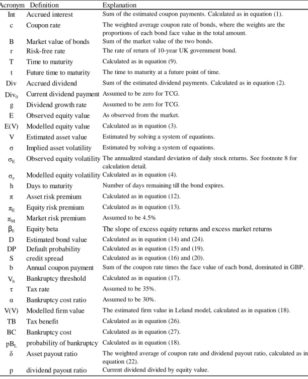
Table 3 Acronyms
This group of acronyms are needed for calibration of the structural models. In the following implementation, the subscript “1” stands for the bond issued in Euro and “2” is the bond issued in GBP. The subscript “M” stands for the values estimated in Merton model while L stands for that of Leland model. The risk-free rates, the market value of equity and bonds are extracted from Datastream.
Acronym Definition Explanation
Int Accrued interest Sum of the estimated coupon payments. Calculated as in equation (1).
c Coupon rate The weighted average coupon rate of bonds, where the weights are the proportions of each bond face value in the total amount.
B Market value of bonds Sum of the market value of the two bonds.
r Risk-free rate The rate of return of 10-year UK government bond.
T Time to maturity Calculated as in equation (9).
t Future time to maturity The time to maturity at a future point of time.
Div Accrued dividend Sum of the estimated dividend payments. Calculated as in equation (2).
Div0 Current dividend payment Assumed to be zero for TCG.
g Dividend growth rate Assumed to be zero for TCG.
E Observed equity value As observed from the market.
E(V) Modelled equity value Calculated as in equation (3).
V Estimated asset value Estimated by solving a system of equations.
σ Implied asset volatility Estimated by solving a system of equations.
σE Observed equity volatilityThe annualized standard deviation of daily stock returns. See footnote 8 for
calculation detail.
σe Modelled equity volatilityCalculated as in equation (4).
h Days to maturity Number of days remaining till the bond expires.
π Asset risk premium Calculated as in equation (12).
πE Equity risk premium Calculated as in equation (13).
πM Market risk premium Assumed to be 4.5%
βE Equity beta The slope of excess equity returns and excess market returns
D Estimated bond value Calculated as in equation (14) and (24).
DP Default probability Calculated as in equation (15) and (19).
S credit spread Calculated as in equation (16) and (20).
b Annual coupon payment Sum of the coupon rate times the face value of each bond, dominated in GBP.
Vb Bankruptcy threshold Calculated as in equation (17).
τ Tax rate Assumed to be 35%.
α Bankruptcy cost ratio Assumed to be 30%.
V(V) Modelled firm value The estimated firm value in Leland model, calculated as in equation (18).
TB Tax benefit Calculated as in equation (26).
BC Bankruptcy cost Calculated as in equation (27).
pBL probability of bankruptcy Calculated as in equation (18).
δ Asset payout ratio The weighted average of coupon rate and dividend payout ratio, calculated as in equation (22).
20
4.1.1 Merton Model
In the structural models, the debt value is the asset value of the firm deducted by the value of equity, which is structured as a call option. In the Merton model, this option has an exercise price of the current market values of the bonds, plus the accrued coupon and dividend payments7. The coupon and dividend payments are assumed to be deferred till the maturity of the bonds and thus their future values grow at the risk-free rate. A list of acronyms is shown in Table 3.
Int = c ∗T
t B ∗ ert (1)
Div = DivT 0(1 + g)t
t ∗ ert (2)
Moreover, the spot price of the underlying asset of this “option” is the implied asset value and therefore in order to obtain the default probabilities and credit spreads, it is required to estimate the asset value, asset volatility and asset risk premium.
E V = VΦ d1 − B + Int + Div e−rTΦ d
2 + Div +IntDiv (V − VΦ k1 +
Div + Int e−rTΦ k
2 ) (3)
σe = σ ∗ [Φ d1 +Div +IntDiv (1 − Φ k1 )] ∗VE (4) where d1 = ln B + Int + DivV + r + σ22 ∗ T σ T (5) d2 = d1− σ T (6) k1 = ln Div + IntV + r + σ22 ∗ T σ T (7) k2 = k1− σ T (8) T = ( B1 B1+ B2∗ h1+ B2 B1+ B2∗ h2)/360 (9)
7 Although TCG has declared dividend in the past, the payments are omitted and thus the initial
21 Objective = (E V E − 1)2+ (σe
σE− 1)
2 (10)
By using Excel solver to solve the system of equation (3) and (4) with the objective to minimize equation (10) 8, the asset value and implied asset volatility are estimated. By minimizing the objective function the modelled asset value (V) and volatility (σe)
could converge with the observed asset value and volatility (σE), and thus the solver
values would be the implied V and σ.
The next step is to have the asset risk premium, which could be calculated using the relationship
σE
σ = πE
π (11)
By rearranging this relationship, π= πE ∗ σ
σE (12)
where
πE = βE ∗ πM9 (13)
So far for the Merton model, inputs for the calculation of debt value (DM), default
probabilities (DPM) and credit spreads (SM) are available. Thus,
DM = V − E(V) (14) DPM = Φ(d2−π T σ ) (15) SM = 1Tln B+IntD M − r (16) 8 σ
E= STD ∗ 262, where STD is the standard deviation of daily stock returns calculated using the
Excel function STDEV and 262 is the number of trading days.
9
The beta is computed as the slope of excess equity returns and excess FTSE 250 returns. Although the choice of market risk premium is debatable in existing studies, it is assumed to be 4.5%, which is widely chosen in empirical tests.
22
4.1.2 Leland Model
For the Leland model, however, as bankruptcy cost and tax benefit are incorporated, and the firm is assumed to pay coupon into infinity, the securities of the firm is structured in a different way. Leland (1994) assumed that bankruptcy is actually determined by shareholders, when the going-concern value of the firm is lower than the firm value if default is executed. Therefore, a bankruptcy threshold (Vb) should be
specified by equity holder, which is calculated as Vb = 1−τ ∗ b
r + σ22 (17)
No model can be accurate and precisely fit into reality, especially when not all of the inputs of the model are directly observable in the market. Thus, the asset value, asset volatility and asset risk premium estimated in section 4.1.1 are taken as the ones for Leland model.
If V is less than Vb, then the equity holders would declare bankruptcy; and if not, the
possibility of shareholders declaring bankruptcy at the time of prediction is measured by the probability of bankruptcy (pBL). Additionally, the default probability (that the
firm would bankrupt at maturity) (DPL) and the credit spread (SL) are calculated as
pBL = (VV b) −2r σ2 (18) DPL = Φ − ln V V b +γT σ T + V Vb −2γ σ2Φ − ln V V b +γT σ T (19) SL = D(V)b − r (20) where γ= π + r − δ −12σ2 (21) and δ =DM V ∗ c + E V∗ p (22)
23
In addition, since Leland model structures firms in a different way, the estimated firm value V(V) is expressed as 𝑉 𝑉 = 𝐷𝐿 + 𝐸𝐿+ 𝑇𝐵 − 𝐵𝐶 (23) where 𝐷𝐿 =𝑏𝑟 + 1 − 𝛼 𝑉𝑏−𝑏𝑟 ∗ 𝑝𝐵𝐿 (24) 𝐸𝐿 = 𝑉 − 1 − 𝜏 𝑏𝑟 + 1 − 𝜏 𝑏𝑟− 𝑉𝑏 ∗ 𝑝𝐵𝐿 (25) 𝑇𝐵 =𝜏𝑏𝑟 (1 − 𝑝𝐵𝐿) (26) 𝐵𝐶 = 𝛼 ∗ 𝑉𝑏 ∗ 𝑝𝐵𝐿 (27) 4.2. Sensitivity Analysis
4.2.1 Hypothesis and Methodology
Table 4
Selected Variables and Hypothesis
Column A is the list of selected variables and the predicted relations of the variables, and default probability and credit spread (signs) are in Column B in accordance with the previous literature review and economic reasoning. The assigned values to each variable in the base case of the sign test are in Column C.
From 2010 to 2013, the business conditions of TCG change dramatically. Therefore it is necessary to conduct a sensitivity analysis to several crucial inputs of the models in order to analyze how the default risk reacts to such changes. The selected variables and predicted signs are presented in Table 4. Throughout the analysis, equity value, annual coupon payment, time to maturity, asset payout ratio and asset beta are constant, tailing to the specific situation of TCG. Then move each variable up or down once at a time so as to have a new default probability and credit spread, and calculated the percentage change.
Variable Predicted sign Assigned value Additional prediction (A) (B) (C) (D)
Volatility (σE) + 100% Positively convex to credit spread
Leverage ratio (B/E) + 2 Risk-free rate (r) - 3% Market risk premium (πM) - 4.5%
Tax rate (τ) - 40% Affect tax benefit and bankruptcy cost Bankruptcy cost (α) + 30% Affect bankruptcy cost
24
In addition to a simple sign test, differences in the percentage trigger further investigation. Reducing the interval of changes, a more precise relationship between the variable and credit spread is illustrated by plotting the variable against credit spread.
4.2.2 Results
Table 5 Sensitivity Analysis
In the computation of new estimates, except for the selected variable and specified changes, other inputs and variables stay constant as in the base case. The methodology is the same as described in section 4.1. The percentile number shown under the new estimates is the percentage change of the dependent variable compared to the original one in base case. If specify, the unit is million of GBP (£M).
In Table 5, it is clear that equity volatility is positively related to default probability and credit spread. The economic reasoning is that as the asset volatility implied by
50% 75% 125% 150% 1 1.5 2.5 3 DPM 0.9025 0.7562 0.8446 0.9414 0.9666 0.8461 0.8832 0.9206 0.9315 -16.21% -6.41% 4.32% 7.11% -6.24% -2.13% 2.01% 3.22% SM 0.4909 0.2925 0.3926 0.5959 0.7104 0.4044 0.4557 0.5273 0.5548 -40.41% -20.04% 21.38% 44.71% -17.64% -7.18% 7.40% 13.01% pBL 0.8164 0.5835 0.7318 0.8677 0.9002 0.8748 0.8742 0.8743 0.8747 -28.53% -10.36% 6.29% 10.27% 7.15% 7.08% 7.10% 7.14% SL 0.1163 0.0344 0.0697 0.1744 0.2425 0.1218 0.1213 0.1217 0.1222 -70.46% -40.11% 49.90% 108.47% 4.74% 4.28% 4.61% 5.02% 2% 2.5% 3.5% 4% 3% 4% 5% 6% DPM 0.9025 0.9055 0.9040 0.9009 0.8993 0.9096 0.9049 0.9000 0.8950 0.34% 0.17% -0.17% -0.35% 0.79% 0.27% -0.27% -0.83% SM 0.4909 0.4950 0.4930 0.4889 0.4870 0.4909 0.4909 0.4909 0.4909 0.83% 0.41% -0.41% -0.81% 0% 0% 0% 0% pBL 0.8164 0.8741 0.8448 0.7888 0.7619 0.8164 0.8164 0.8164 0.8164 7.07% 3.49% -3.38% -6.67% 0% 0% 0% 0% SL 0.1163 0.1214 0.1188 0.1139 0.1114 0.1163 0.1163 0.1163 0.1163 4.33% 2.15% -2.12% -4.21% 0% 0% 0% 0% 30% 35% 45% 50% 20% 25% 35% 40% pBL 0.8164 0.8248 0.8207 0.8117 0.8065 0.8164 0.8164 0.8164 0.8164 1.03% 0.53% -0.58% -1.21% 0% 0% 0% 0% DPL 0.4382 0.4720 0.4557 0.4195 0.3993 0.4382 0.4382 0.4382 0.4382 7.72% 3.99% -4.28% -8.89% 0% 0% 0% 0% SL 0.1163 0.1197 0.1181 0.1143 0.1121 0.1142 0.1152 0.1174 0.1185 2.89% 1.53% -1.71% -3.62% -1.85% -0.93% 0.95% 1.91% Vb (£M) 57.29 66.84 62.06 52.52 47.74 57.29 57.29 57.29 57.29 16.67% 8.33% -8.33% -16.67% 0% 0% 0% 0% DL(£M) 313.49 306.46 309.73 317.80 322.77 318.17 315.83 311.15 308.81 -2.24% -1.20% 1.38% 2.96% 1.49% 0.75% -0.75% -1.49% EL(£M) 989.36 961.94 975.49 1,003.57 1,018.16 989.36 989.36 989.36 989.36 -2.77% -1.40% 1.44% 2.91% 0% 0% 0% 0% TB(£M) 112.30 80.36 95.93 129.58 147.91 112.30 112.30 112.30 112.30 -28.44% -14.58% 15.39% 31.71% 0% 0% 0% 0% BC(£M) 14.03 16.54 15.28 12.79 11.55 9.35 11.69 16.37 18.71 17.87% 8.91% -8.86% -17.67% -33.33% -16.67% 16.67% 33.33% r πM τ α Base σE B/E
25
equity volatility becomes higher, the higher the uncertainty of TCG failing to repay debt, and thus the default probability increases and investors would ask for more compensation for bearing such risk. Moreover, although it is hypothesized that volatility is positively convex against credit spread, in Figure 3 and 4 it seems that for
Figure 3
Volatility against Credit Spread in the Merton Model
Holding other inputs constant, the credit spread is calculated by moving the equity volatility 10% at a time stating from 30% till 200%. The relationship is almost linear.
Figure 4
Volatility against Credit Spread in the Leland Model
Similar with Figure 3, the interval of changes is 10%. The relationship between equity volatility and credit spread is slightly more convex than that of Figure 3, but not evident.
0% 20% 40% 60% 80% 100% 120% 30% 70% 110% 150% 190%
S
M σE 0% 10% 20% 30% 40% 50% 30% 70% 110% 150% 190% SL σE26
TCG the relationship of volatility and credit spread is not obviously convex, and is almost linear in the Merton model.
Figure 5
Leverage against Credit Spread in Merton model
The interval of changes in debt-to-equity ratio (B/E ratio) is 0.25 from 0.5 to 3.5. The relationship between leverage ratio and SM is positive as predicted.
Figure 6
Leverage against Credit Spread in Leland model
Similar with Figure 5, SL is calculated by moving the B/E ratio 0.25 at a time. The
relationship is U-shaped, meaning that under the assumptions of Leland model, the credit spread could be minimized by altering the leverage ratio.
30% 35% 40% 45% 50% 55% 60% 0.5 1 1.5 2 2.5 3 3.5 SM B/Eratio 11.4% 11.5% 11.6% 11.7% 11.8% 11.9% 12.0% 0.5 1 1.5 2 2.5 3 3.5 SL B/E ratio
27
The most interesting finding lies in the analysis of leverage ratio. Illustrated in Figure 5, leverage ratio is positively associated with SM; whereas in Figure 6 the relationship
between B/E ratio and SL is U-shaped, which explains why in Table 5 the percentage
changes of pBL and SL with B/E ratio are both positive in either direction of changes.
Since tax benefit and bankruptcy cost are incorporated into the Leland model, it is possible that there exist an optimal capital structure that could minimize the credit spread. For TCG, the optimal leverage ratio lies in the range of 1.5 to 2.
The risk-free rate is negatively related to default probability and credit spread in both models, which is also in line with previous literature. The relationships between r and the default probability and credit spread are linear, which is confirmed in Figure 7 and 8. Besides, the steeper slope of SL demonstrates that the Leland model is more
sensitive to a change in risk-free rate. Notice that both SM and SL are considerably
higher than the presumed r. As a result, it may be that for TCG, especially with Merton model, the variation of risk-free rate is not a major determinant in accessing credit risk.
Judging from the percentage changes in Table 5, the choice of market risk premium only affects the levels of DPM, and the influence is minor. Although the equity
premium of companies with B-rated bonds is suggested to be 8.76% in Huang and Huang (2003), it is calculated using the capital asset pricing model (CAPM) in this paper. Thus it is more likely that the equity premium and default probability are subjected to the riskiness (beta) of the securities.
As predicted, the tax rate is negatively associated with default probability and credit spread in the Leland model, suggesting the tax effect. Normally holding the debt level constant, a higher tax rate may help the company further exploit the tax benefit and thus would raise the total firm value and lower the bankruptcy threshold Vb. However
for TCG, the effective tax rate increases mainly caused by low profit level. Hence, the tax benefit would be counterbalanced by the effect of weakening profitability.
Shown in Table 5, the bankruptcy cost ratio, nonetheless, seems to have minor impact onto the assessment of credit risk in this sensitivity analysis. The linear relationship between α and DL is straightforward in equation (24), and thus it would affect the
credit spread. With respect to the economic reasoning, it may be that bankruptcy cost is a factor of estimated firm value V(V), and affects the asset level once the firm is
28
pushed to debt holders. Hence, α may play a role in valuation but not in accessing credit risk.
Figure 7
Risk-free Rate against Credit Spread in the Merton Model In the Merton model, the relationship of r and SM is negative as forecasted, and is linear.
Figure 8
Risk-free Rate against Credit Spread in the Leland Model
SL is also negatively related to r. Additionally, the range of variation in SL is larger than that
of SM, when r is moving from 1.5% to 5%.
47.5% 48.0% 48.5% 49.0% 49.5% 50.0% 1.5% 2.5% 3.5% 4.5% SM r 9.0% 10.0% 11.0% 12.0% 13.0% 1.5% 2.5% 3.5% 4.5% SL r
29
4.3 Empirical findings
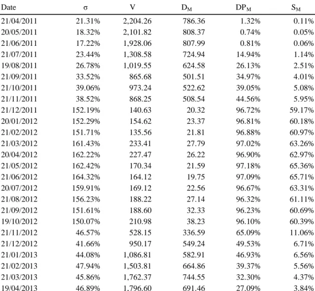
Table 6 Merton Model
The default probabilities and credit spreads are calculated on a monthly basis, using the data of 262 trading days before the date of estimation. The date of estimation is the business day that is closest to and before 21st of each calendar month from April 2011 to April 2013. The unit for V and DM is million of GBP.
Note that the market capitalization of TCG suddenly dropped below £750 million in the middle of July 2011 and remained below 300 million from November 2011 till the end of 2012. Since the estimations use the stock values of 262 trading days prior to the date of prediction, this period of recession accounts for the sudden increases in asset volatilities and declines in asset values, resulting in high levels of default probabilities and credit spreads.
The results for Merton model are shown in Table 6. Initially from April to June 2011 the estimated bond value is higher than the face value of issued bonds and thus the predicted probabilities of default are low and the credit spreads are approximately or below 0.1%. Since July 2011 the implied asset volatilities have increased, resulting in increasing default probabilities and the credit spreads. Affected by the depression in the market and declining profit level, the stock prices for TCG suddenly decreases to
Date σ V DM DPM SM 21/04/2011 21.31% 2,204.26 786.36 1.32% 0.11% 20/05/2011 18.32% 2,101.82 808.37 0.74% 0.05% 21/06/2011 17.22% 1,928.06 807.99 0.81% 0.06% 21/07/2011 23.44% 1,308.58 724.94 14.94% 1.14% 19/08/2011 26.78% 1,019.55 624.58 26.13% 2.51% 21/09/2011 33.52% 865.68 501.51 34.97% 4.01% 21/10/2011 39.06% 973.24 522.62 39.05% 5.08% 21/11/2011 38.52% 868.25 508.54 44.56% 5.95% 21/12/2011 152.19% 140.63 20.32 96.72% 59.17% 20/01/2012 152.29% 154.62 23.37 96.81% 60.18% 21/02/2012 151.71% 135.56 21.81 96.88% 60.97% 21/03/2012 161.43% 233.41 27.79 97.02% 63.26% 20/04/2012 162.22% 227.47 26.22 96.90% 62.97% 21/05/2012 162.42% 170.34 21.59 97.18% 65.36% 21/06/2012 164.32% 164.12 19.75 97.09% 65.71% 20/07/2012 159.91% 169.12 22.56 96.67% 63.31% 21/08/2012 156.23% 188.22 27.14 96.32% 61.11% 21/09/2012 151.61% 188.60 32.33 96.23% 60.69% 19/10/2012 150.07% 210.98 38.23 96.10% 60.39% 21/11/2012 46.57% 528.15 336.59 65.09% 11.06% 21/12/2012 41.66% 950.17 549.24 49.53% 6.71% 21/01/2013 44.08% 1,086.81 582.91 46.93% 6.56% 21/02/2013 47.94% 1,503.81 664.86 39.37% 5.56% 21/03/2013 45.86% 1,762.37 744.55 32.30% 4.37% 19/04/2013 46.89% 1,796.60 691.46 27.09% 3.84%
30
60p in July 2011, which dramatically raises the asset volatility to over 150%. The default probabilities and credit spreads for December 2011 to October 2012 remain as high as 97% and over 60% respectively. Indeed, despite some organizational changes since 2011, the capital refinancing at the beginning of 2013 is considered to be a default event, meaning that the Merton model successfully anticipate default. After business reconstruction and recapitalization, the financial health of TCG is gradually recovered, and the asset volatilities and default probabilities declines but are consistently high.
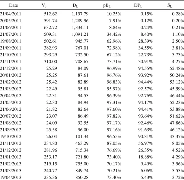
Table 7 Leland Model
Consistent with Table 6, the estimates are presented on a monthly basis. Additionally, the jumps in the market value of equity may account for the sudden plumps in the value of bankruptcy threshold and thus largely inflate the default probabilities and credit spreads. The units for Vb and DL are million of GBP.
Date Vb DL pBL DPL SL 21/04/2011 512.62 1,197.79 10.25% 0.15% 0.28% 20/05/2011 591.74 1,289.96 7.91% 0.12% 0.20% 21/06/2011 632.72 1,334.11 8.84% 0.24% 0.21% 21/07/2011 509.31 1,091.21 34.42% 8.40% 1.10% 19/08/2011 502.61 945.77 62.96% 28.39% 2.50% 21/09/2011 382.93 767.01 72.98% 34.55% 3.81% 21/10/2011 293.29 732.50 67.12% 22.73% 3.73% 21/11/2011 310.00 708.67 73.71% 30.91% 4.27% 21/12/2011 25.29 84.09 96.99% 94.55% 52.48% 20/01/2012 25.25 87.61 96.76% 93.92% 50.24% 21/02/2012 25.42 82.89 96.83% 94.44% 53.12% 21/03/2012 22.49 95.81 95.97% 92.57% 45.59% 20/04/2012 22.31 94.53 96.39% 92.76% 46.44% 21/05/2012 22.30 84.94 97.31% 94.17% 52.23% 21/06/2012 21.82 82.64 97.60% 94.41% 53.88% 20/07/2012 23.07 86.49 97.82% 93.64% 51.62% 21/08/2012 24.09 92.55 97.17% 92.46% 47.86% 21/09/2012 25.58 96.00 97.16% 91.63% 46.12% 19/10/2012 26.04 101.34 96.55% 90.31% 43.37% 21/11/2012 234.80 463.29 87.05% 56.97% 8.05% 21/12/2012 281.96 715.34 76.69% 26.35% 4.52% 21/01/2013 253.17 721.80 73.40% 18.88% 4.29% 21/02/2013 219.15 755.00 70.17% 9.49% 3.96% 21/03/2013 240.77 849.74 70.21% 6.06% 3.53% 19/04/2013 235.36 850.28 73.40% 5.43% 3.72%
31
Table 7 shows the Leland model results. pBL measures the probability of equity
holders declaring bankruptcy prior to maturity, which is also a discounting factor in estimating the value of debt, equity, tax benefit and bankruptcy cost. Even though in Leland model the liabilities of firms are treated as perpetual bonds with fixed coupon payments, the default probabilities (DPL), of which the definition is comparable to
that in the Merton model, are also presented.
Overall the Leland model demonstrates similar patterns and trends with the Merton model. Both pBL and DPL are low from April to June 2011 but increase during the
following quarter and reach the peak in the middle of 2012. After November 2012 the DPL drops down to below 10% while pBL slightly fluctuates around 70%. The credit
spreads have same pattern of the default probabilities, that is, the spreads are low when the possibilities are low and also change dramatically when there are sudden jumps in asset values. This supports that the Leland model can also provides useful information for default forecast.
Notice that in Table 7 the Vb on November 2012 is almost 10 times of the previous
month. Also, the implied asset values V in Table 6 bounce back at the beginning of FY2013. Indeed, this is when TCG continues to lower net debt and has the equity injection and new bond issue fully underwritten. The market data and modelled statistics reflect such information.
4.4 Comparative analysis
Figure 9 shows that DPM, DPL and pBL generally share the same trend. In terms of
levels, DPL is lower than DPM and pBL is highest of all. This indicates that in
financially distressed firms like TCG, it is the owners rather than the creditors who have a higher incentive to vote for bankruptcy. Hence, such a gap is reasonable owing to the different underlying assumptions. Nevertheless, these results prove that both Merton model and Leland model are successful in terms of predicting bankruptcy and accessing default possibilities, which is line with the previous empirical findings. Figure 10 compares the predicted credit spreads calculated in the two models. Interestingly, SM is lower than SL from April to August 2011, when the firm is
financially healthier and the risk-free rate is higher, but higher than SL since then as