Deterministic tsunami hazard assessment of Sines - Portugal

2015

FACULDADE DE CIÊNCIAS

DEPARTAMENTO DE ENGENHARIA GEOGRÁFICA, GEOFÍSICA E ENERGIA

Deterministic Tsunami Hazard Assessment of Sines - Portugal

Mestrado em Ciências Geofísicas

Oceanografia

Martin Wronna

Dissertação orientada por:

Prof. Doutor Jorge Miguel Alberto de Miranda, Profª Doutora Maria Ana de Carvalho Viana

Baptista

Abstract

This study employs a deterministic approach for multiple source tsunami hazard assessment for the city and harbour of Sines – Portugal, one the test-sites of project ASTARTE. Sines holds one of the most important deep-water ports which contains oil-bearing, petrochemical, liquid bulk, coal and container terminals. The port and its industrial infrastructures are facing the ocean southwest towards the main seismogenic sources. This work considers two different seismic zones: the Southwest Iberian Margin and the Gloria Fault. Within these two regions, we selected a total of six scenarios to assess the tsunami impact at the test site. The deterministic approach consists in solving linear and non-linear shallow water equations using an explicit leap-frog scheme to obtain water elevations in predefined grids for a defined time step. Numerical model computation process is launched after defining an initial seafloor displacement on a prepared set of nested grids. The Digital Elevation Model includes bathymetric and topographic information with 10m resolution in the study area. To do the tsunami simulations a Non-linear Shallow Water Model With Nested Grids – NSWING is used. In this study, the static effect of tides is analysed for three different tidal stages. Tsunami impact scenarios are described in terms of inundation area, maximum values of wave height, flow depth, drawback, run-up and inundation distance. Synthetic waveforms are computed for virtual tide gauges at specific locations outside and inside the harbour. The final results describe the impact at Sines test site considering the different source scenarios at mean sea level, the aggregate scenario and the influence of the tide on the aggregate scenario. The results confirm the composite source Horseshoe and Marques Pombal fault as the worst case tsunami scenario. It governs the aggregate scenario with about 60% and inundates an area of 3.5km².

Key-words: Deterministic tsunami hazard assessment, numerical modelling, aggregate scenarios, integrated hazard maps.

Resumo

Neste trabalho apresenta-se uma abordagem determinística de perigo de tsunamis considerando múltiplas fontes para a cidade costeira de Sines, Portugal. Tsunamis ou maremotos são eventos extremos, energeticamente elevados mas pouco frequentes. Normalmente são geradas por um deslocamento duma grande quantidade de água seja por erupções volcánicas, collapse de caldeiras, deslizamentos de massa, meteorites ou terramotos submarinos. A grande maioria é causado pelos terramotos submarinos. Neste trabalho estuda-se sómente efeitos causado por tsunamis gerados pelos deslocamentos de solo submarino devido a terramotos. O evento no oceano Índico em 2004 demonstrou a necessidade de um sistema de alerta operacional global. E o Tohoku terramoto em 2011 moustrou as limitações do conhecimento científico respetivamente às zonas fontes, os impactos costeiros e medidas de mitigação. A partir desta data na zona Noreste Atlantico e Mediterrâneo e mares adjacentes (NEAM) esforços foram feitos para melhorar as capacidades de avaliação de perigo de tsunamis. Em Portugal a zona considerada mais ativa é o Golfo de Cadiz. Relatos históricos antigos voltam atrás até 60 BC, mas evidências geológicas mostram eventos energeticamente elevadas até 218 BC.

A costa portuguesa é altamente exposta ao perigo de um tsunami a partir de fontes tectónicas ativas locais e regionais. A zona principal tsunamigenica é o SWIM (Margem sudoeste da Península Ibérica), que inclui numerosas falhas inversas que mergulham em direcção sudeste. O evento mais rigoroso foi o 1º Novembro 1755 causado pelo famoso terramoto de Lisboa com mais do que dez mil vítimas mortais e uma magnitude estimada de 8.5. A fonte do tsunami ainda não é conhecida definitivamente, pois na altura ainda não havia instrumentos para registrar sismos. A fonte foi aproximada por diferentes autores utilizando as informações históricos e assuma-se que é localizada na zona SWIM. O impacto do tsunami ocorreu na bacia inteira do ocenao Atlântico Norte com maior impacto na Ibéria e em Moroccos. No seculo 20 no dia 28 de Fevereiro 1969 um sismo de magnitude 7.9 causou um tsunami pequeno com uma amplitude de 0.5m em Lagos e Cascais. As ondas aproximaram-se da costa por volta das 3 de manha em condições maré vazia e não causaram danos significativos.

O trabalho foi desenvolvido no ambito do projeto ASTARTE [Grant 603839]. Em Sines encontra-se um dos portos mais importantes de agua profunda de Portugal contenido terminais petrolíferos, petroquímicos, graneis líquidos, carvão e contentores. O porto está ligado aos centros industriais em Sines com infraestruturas frageis como gasoduto, oleodutos, tanques de gás natural liquefeito ou cinturões industriais, quais ocorrem o risco de ser danificados. Possiveis danos geram riscos addicionais como explusões ou poluições ambientais. Na zona sul da area do estudo encontra-se o central thermoeletrico da EDP que utliza a água do mar pelo arrefecimento dos geradores. Sines também e um destino turístico com um porto de recreio e com varias praias associadas aos desportos náuticos como a pesca deportiva, a vela, o mergulho e o surf. A zona de estudo inclui o porto de recreio e as praias de Vasco da Gama e de São Torpes. O porto, o central thermoelétrico e as suas infrastruturas industriais e as praias enfrentam ao Atlantico a sudoeste direcionado às zonas principais de rupturas sísmicas consideradas suficientemente fortes de causar tsunamis e por causa disso a zona de estudo escolhido é altamente exposto ao perigo dum tsunami. Foram consideradas as zonas de fontes a falha da Gloria (GF) e a zona da margem sudoeste da península Ibérica (SWIM) e cinco falhas diferentes, nomeadamentes: A falha da Gloria que é uma falha de cisalhamento que defina a fronteira entre Eurasia e Nubia; a falha de Cadiz Wedge (CWF) que é considerada como uma zona de subducção e as falhas do banco de Gorringe (GBF), de Ferradura (HSF) e de Marques Pombal (MPF) que são falhas inversas que mergulham em direcção sudeste. Adicionalmente foi considerado uma combinação da falha de ferradura e da falha Marques Pombal (HSMPF) para a simulação. Um ruptura simultânea de falhas com parâmetros parecidos foi proposta por varios autores como uma possível fonte do tsunami em 1755. A zona SWIM é considerado uma zona complexa em termos geodinâmicos onde varios processos atuam simultaneamente. Para cada falha identificada e para a combinação HSMPF o pior dos cenários sísmicos foi assumido para o procedimento da modelação numérica.

A abordagem deterministica consiste em resolver as equações lineares e não-lineares de água pouca profunda para puder obter as elevações da superfície livre do oceano em cada passo tempo definido. As equações de água pouca profunda são válidas devido do facto que tsunamis são ondas longas. Ondas são consideradas longas quando o seu comprimento de onda 𝜆 é muito maior que a altura de coluna de agua ℎ ou quando se verifica ℎ

𝐿< 1

Na simulação numérica da propagação do tsunami é utilizado modelo NSWING (Non-linear Shallow Water Model with Nested Grids) (Miranda et al., 2014) que resolve as equações de água pouca profunda utilizando um esquema “leap-frog” explícito para os termos lineares e um esquema “upwind” para os termos não-lineares. Após definir o deslocamento inicial do fundo do oceano o modelo calcula as soluções para cada cenário dentro de um sistema de grelhas encastradas. Para poder calcular os deslocamentos iniciais aplicando a teoria de inelasticidade de Okada (1985) foram utilizados parâmetros presentados de campanhas e estudos recentes. Foi aplicado uma distribuição dum slip não uniforme onde o slip defina o deslocamento inicial em cada célula da grelha. Este deslocamento inicial e traduzida pela superfície livre onde o processo numérico da propagação do modelo começa e as equações de água pouca profunda são resolvidas em cada passo tempo para cada célula de sistema de grelhas ligadas. Neste estudo o sistema das grelhas encastradas ou “nested grids” consiste num conjunto de quatro grelhas ligadas. Na zona fonte e em oceano aberto utiliza-se uma grelha com células maiores. Células de 640x640m reduzindo-as para 10x10m quando se atinge a zona de estudo. Usam-se duas grelhas intermédias 160m e 40m aplicando um fator de refinamento de 4. Para puder analisar efeitos locais com essa resolução alta precisa-se um DEM (modelo digital de terreno) com informações detalhadas sobre a bathimetria e a topografia da area de estudo. O DEM foi elaborado utilzando um conjunto de dados do Instituto Hidrográfico de Portugal e da Direção-geral do Território num SIG (sistema de informação geográfica). A inundação é obtida a partir dum algoritmo designado “moving boundary-percurso da linha de costa” baseado em células secas e células inundadas para conseguir seguir a linha da costa (Liu et al., 1995).

Também foi considerado o efeito da maré. Os valores de maré cheiá foram obtidos calculando a média das médias de todas as Preias-mar e da maré vazia a média das médias de todas as Baixas-mar de 2012 até 2014. Para cada cenário foram calculadas três condições de maré, da condição maré cheia, do nivel médio do mar e da condição maré vazia.

Os resultados finais são apresentados em forma de mapas integrados de perigo para cada cenário considerado e para o cenário agregado. Cada mapa integrada de perigo consiste em valores máximos de altura de onda (MWH), profundidade de fluxo (MFD), recuo (MDB), runup (MRU) e distância de inundação do cenário correspondente. Formas de ondas sintéticas foram calculadas em pontos da grelha designados por marégrafos virtuais em pontos representativos dentro e fora do porto. Os resultados finais descrevem o impacto em Sines considerando cada único cenário de nível médio do mar, o cenário agregado e a influência da maré no cenário agregado. Os resultados confirmam que o pior caso cenário é a combinação da falha de ferradura e da falha Marques Pombal HSMPF. Este cenário domina o cenário agregado com aproximadamente 60% e inunda uma área de 3.5km².

Palavras-chave: Abordagem determinística do perigo de tsunami, modelação numérica, cenários agregados, mapas de perigo integrados.

Acknowledgements

I would like to thank Maria Ana Baptista, Jorge Miguel Miranda and Rachid Omira for their great support and fruitful discussions throughout the entire investigation process, Carlos Antunes for providing the GPS RTK equipment of Lisbon Faculty of Sciences, Commandant José Brazuna Fontes of Sines harbour for his support for the field survey and Direção Geral do Território for making available LIDAR data of the study area.

I wish to express my thanks to my family for their support, especially my parents Ursula and Günter Wronna, my sister Edith Wronna, my Grandmother Christine Achleitner and my aunt Gertrude Kneissl. And I wish to express my gratefulness to my girlfriend Maria Fuchs for her patience and mental motivation. Additionally I want to thank my friends Daniela, Joana, Laura, Susana, Alessandro, Carlos and Miguel who supported me throughout the master classes.

Index

Abstract ... iii

Resumo ... iv

Acknowledgements ... vi

Index ... vii

List of figures ... viii

List of tables ... ix

1. Introduction ... 1

1.1. Wave and Tsunami physics ... 4

1.2. Geoscientific context ... 9

2. Methodology ... 13

2.1. Preparation of the tsunami simulation ... 13

2.2. Generation of tsunamis in the source area ... 15

2.3. Digital Elevation Model ... 17

2.4. Tsunami Propagation & SWEs ... 18

2.5. Tsunami inundation & Run up ... 20

3. Application ... 22

4. Discussion ... 39

5. Conclusion ... 41

List of figures

Figure 1.1 Schematic illustration of physical quantities such as amplitude, wave height, flow depth, run up and inundation distance referenced to a given sea level. ... 2 Figure 1.2 Schematic sketch of the simplified conditions of waves propagating in x-direction; modified from Sorensen (2006). ... 5 Figure 1.3 Illustration of wave condition depending on wave length and water depth (Bowden, 1983). 8 Figure 1.4 A: ATJ – Azores triple junction; AGFZ Azores-Gibraltar fracture zone B: Tectonic map of southwest Iberian Margin (SWIM). Grey arrows show Gibraltar Arc westward movement; white arrows show Africa-Eurasia WNW-ESE convergence. Modified from Duarte et al. (2013) ... 12 Figure 2.1 Schematic outline of the 4 Layer prepared for NSWING; Layer 41 contains the DEM. .... 14 Figure 2.2 Definition of an individual seismogenic source. (Istituto Nazionale di Geofisica e Vulcanologia, 2015) ... 16 Figure 2.3 Resulting digital elevation model (DEM) of Sines test-site. ... 17 Figure 2.4 Illustration of the inundation algorithm in one dimension as presented in Liu et al. (1998) and Wang (2009) for 2 cases and MWL is the Mean Water Level. ... 21 Figure 3.1 (a) General map: Location of Sines test site; (b) test site map identifying general features and tide gauges for synthetic wave forms. ... 24 Figure 3.2 TFs used for Tsunami modeling in the SWIM. Dextral reverse faults: Gorringe Bank fault (GBF), Marques Pombal fault (MPF), Horseshoe fault (HSF); Subduction slab: Cadiz Wedge Fault (CWF). ... 27 Figure 3.3 Dimension and geographic location of the Gloria fault (red line) considered in this study. 28 Figure 3.4 Results of MWH, MFD, MDB and MRU of the SWIM scenarios considering MSL: (a) CWF, (b) GBF, (c) HSF, (d) HSMPF, (e) MPF. ... 29 Figure 3.5 Synthetic waveforms for 6h propagation time at 3 chosen points (cf. Fig. 3.1) for the SWIM scenarios: (a) CWF, (b) GBF, (c) HSF, (d) HSMPF, (e) MPF. ... 30 Figure 3.6 (a) Results MWH, MFD, MDB and MRU for the Gloria scenario, (b) synthetic waveform for 6h propagation time a 3 chosen points (cf. Fig. 3.1) for the Gloria scenario. ... 31 Figure 3.7 MWH, MFD, MDB and MRU for the aggregate scenario considering all stages of the tide.

... 32 Figure 3.8 MDB and MRU limits for the stages MLLW, MSL and MHHW of the tide. ... 33 Figure 3.9 Contribution of individual scenarios to the aggregate model at MSL. ... 34

List of tables

Table 1.1 Basic terms and definitions used in this thesis. ... 1 Table 3.1 Fault parameters of the tsunamigenic sources considered in this study. ... 28 Table 3.2 Synthesis of the Results: MFD, MWH, inundated area, MDB, MRU and arrival time for all scenarios at MSL. ... 31 Table 3.3 Contribution of the scenarios to the aggregate model considering 3 stages of the tide. ... 34

1. Introduction

Tsunamis are low frequency but high impact hazards for coastal societies. Tsunamis are sets of waves produced by an abrupt displacement of a large amount of water. Generating processes are usually geologic activities such as earthquakes, volcanic eruption or landslides. Rare meteorite impacts extreme meteorological events for example abrupt atmospheric pressure jumps may also cause Tsunamis. The term tsunami originates from the Japanese “tsu” what means harbour and “nami” what means wave. Fisherman used it to describe flooding waves that sometimes destroyed the harbours. Submarine earthquakes trigger the great majority of tsunamis. Also from distant sources their impact can be tremendous. But not all submarine earthquake cause tsunamis only those that produce sufficient vertical seafloor deformation and dislocate the entire water column above. To prepare and protect coastal societies it is fundamental to understand better their impact at coastal shorelines. To understand better their nature scientists run numerical models to take precautions.

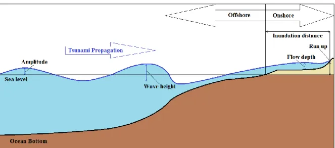
Basic terms and physical quantities used in the thesis are presented in table 1.1. Some physical quantities mentioned are depicted in Fig. 1.1.

Table 1.1 Basic terms and definitions used in this thesis. Amplitude: Height of the crest of the tsunami above mean sea level.

Bathymetry: The measurement of the depth of the ocean floor from the water surface. Topography: The measurement of the elevation of the land surface from the sea level. Wave Height: The wave height is measured as the difference between wave crest and

trough in a certain point.

Flow Depth or Inundation Depth: Depth or height of the tsunami above the ground in the inundation zone. It measures the thickness of the water layer on land.

Inundation or inundation distance: The horizontal distance in land that a tsunami penetrates; is measured perpendicular to the shoreline.

Maximum inundation area: Maximum horizontal penetration of the tsunami inland

Mean Lower Low Water (MLLW): The average of all the lower low water heights over a specific period.

Mean Sea Level (MSL):

The MSL is given by the arithmetic mean of hourly heights of tide height on the open coast or in adjacent waters which have free access to the sea, observed over a specific time period. The MSL is often used as geodetic datum.

Mean Higher High Water (MHHW): The average of all the higher high water heights over a specific period. Maximum Drawback: The maximum drawback gives the maximum area that remains dry

offshore as the result of the tsunami arrival in the test site.

Run Up:

The maximum water elevation within the limit of inundation; this is usually greater than the wave amplitude at the coast. The run up height (or the elevation reached by the seawater) is measured relative to some given reference datum. In most studies and is referenced to MSL. In this thesis Run Up is referenced to MLLW, MSL or MHHW depending on the tide considered.

Period: Time interval between two consecutive wave crests or troughs.

Recurrence or Return Period:

An interval of time long enough to encompass many events divided by the number of events equal or greater than a specific magnitude that are expected to occur.

Tsunami Travel Time: Time required for the first tsunami wave to propagate from its source to a given point on a coastline.

Figure 1.1 Schematic illustration of physical quantities such as amplitude, wave height, flow depth, run up and inundation distance referenced to a given sea level.

The 26th December, 2004 Indian Ocean and the 11th March, 2011 Tohoku-Oki striking tsunami events raised awareness due to the enormous loss of life and property. The Indian Ocean event in 2004 demonstrated the need for operational early warning systems around the world. However, seven years later, the 2011 Tohoku-Oki event showed the limitations of the scientific knowledge concerning tsunami sources, coastal impacts, and mitigation measures. Since then, in the NEAM region (North East Atlantic, Mediterranean and connected seas) many efforts have been addressed to understand better the tsunamigenic sources and to improve the tsunami hazard assessment capabilities. Within the NEAM region, the Gulf of Cadiz is among the most tsunami hazardous areas. The historical reports include events dated back to 60 BC (Mendonça, 1758, Baptista and Miranda, 2009; Kaabouben et al., 2009). However, the geological evidence indicates that high energy events occurred back to 218 BC (Luque et al., 2001).

This study was developed in the framework of ASTARTE project “Assessment, STrategy And Risk Reduction for Tsunamis in Europe” [Grant 603839]. The project uses nine test sites in the North East Atlantic and Mediterranean (NEAM) Region. The test site selection considered that:

 Test sites can be impacted by regional and local tsunami sources, which put different levels of stress on detection and forecasting

 Different tsunami source types, such as earthquakes, landslides, volcanoes and rockslides, some of which not included in NEAMTWS

 Different values at risk including industry, harbours and other infrastructures, and ecosystems

 Different coastal communities such as fishing communities, coastal cities and tourist developments

 Test sites include a broad geographical coverage, in both North-east Atlantic and Mediterranean coasts

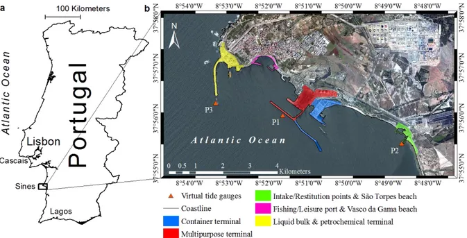
In Portugal the test site is the city of Sines. The study area consists of different topographic features like beaches, rocks, rocky outcrops, plains and smaller river course valleys and is interfered by big harbour and industrial structures.

The Portuguese coast is exposed to tsunami threat from local and regional tectonic sources (Intergovernmental Oceanographic Commission, 2013). The main tsunamigenic area is the SWIM (South West Iberian Margin), with some considerable SE dipping inverse faults (Zitellini et al., 2009, Matias et al., 2013). The most severe tsunami occurred on November 1st 1755. The tsunami followed the Lisbon earthquake with an estimated magnitude of 8.5 by Martins and Mendes Victor (1990). The

magnitude was more recently re-evaluated by Solares and Arroyo (2004) with an estimate of 8.5±0.3. The tsunami hit the entire northern Atlantic basin with huge impact in Iberia and Morocco (Baptista and Miranda, 2009). In the 20th century, the February 28th, 1969 earthquake with a magnitude of 7.9 (Fukao, 1973) caused a small tsunami of 0.5 m amplitude in Lagos and Cascais (Baptista et al., 1992; Baptista and Miranda, 2009). The tsunami waves hit the coast in low tide conditions at circa 3 a.m. (Baptista et al., 1992) and no significant damage was observed.

The second tsunamigenic zone to be considered is the Gloria Fault. The Gloria fault is a segment of the Eurasia-Nubia plate boundary. It is a large strike slip fault, located between 24ºW and 19ºW, with scarce seismic activity. Nonetheless, this area was the location of several large events during the 20th Century, in particular the November 25th, 1941 earthquake, a submarine strike-slip event of magnitude 8.3-8.4 (Gutenberg and Richter, 1949) and the May 26th, 1975 with magnitude 7.9 (Lynnes and Ruff, 1985; Grimson and Chen, 1986).

In recent years, a considerable number of tsunami hazard assessment studies were published for the North East Atlantic area. Most studies focus on the tsunami impact in the Gulf of Cadiz using a scenario based or deterministic approach, namely: Lima et al. (2010), Omira et al. (2010), Omira et al. (2011), Atillah et al. (2011), Baptista et al. (2011a), Renou et al. (2011), Omira et al. (2013), Benchekroun et al. (2013) and Lemos et al. (2014).

Actually, two different assessment methods are used to study the tsunami impact at a certain test site, the PTHA (Probabilistic Tsunami Hazard Assessment) and DTHA or SBTHA (Deterministic Tsunami Hazard Assessment or Scenario Based Tsunami Hazard Assessment).

The PTHA approach consists in considering the recurrence rates of earthquake scenarios with different magnitudes. By knowing the recurrence rates of the different magnitude scenarios a database is generated using numerical modelling methods. Apart from this results a probability exceeding a certain wave height/flow depth in a given period is assessed. Recently, Omira et al. (2015) published a probabilistic tsunami hazard assessment for the North East Atlantic. These studies gain in reliability the longer the geological databases reach back. Another method used in PTHA is to apply an aleatory statistical tool called Monte Carlo simulations (e.g. Ten Brink et al., 2009, Grilli et al., 2009, Sørenson et al., 2012).

The DTHA or SBTHA methodology consists of studying the impact of specific tsunami events – tsunami scenarios - in the study area. Usually the specific tsunami events are based on geological information considering the Maximum Credible Earthquake (MCE) scenario or the Worst-case Credible Tsunami Scenarios (WCTS) considering the typical fault (TFs) of the source zones in the study area. Numerical simulation of the chosen scenarios calculates the tsunami impact in the test-site. By estimating parameters as wave height, flow depth, drawback, inundation distance hazard maps are elaborated. This methodology has been applied to assess tsunami hazard around the globe (e.g. Baptista et al., 2011a, Tonini et al., 2011, Mitsoudis et al., 2012, Phuong et al., 2014, Wijetunge, 2014). The deterministic approach is more suitable to establish tsunami mitigation measures and coastal municipality authorities.

In this master thesis, the DTHA approach has been used to evaluate the tsunami impact in Sines. The impact is described in terms of maximum wave height (MWH), maximum flow depth (MFD), maximum run up (MRU) and maximum drawback (MDB). Further the aggregate scenario has been built plotting the MWH in each cell considering the contribution of the individual scenarios (Tinti et al., 2011).The study area contains the country’s most important deep water port that is connected to big industrial complexes by fragile infrastructure such as pipelines and conveyor belts. In summer the city is a popular tourist destination.

The final results are presented in integrated hazard maps for all the considered and the aggregate scenario. Each integrated hazard map consists of MWH, MFD, MRU and MDB of the corresponding scenario. The analysis of tide effect consists of three different tidal stages mean lower low water (MLLW), mean sea level (MSL), and mean higher high water (MHHW). Further the contribution of each scenario to the aggregate tsunami impact is presented at MSL condition.

1.1. Wave and Tsunami physics

In this master thesis the focus has been laid on studying the hazard of earthquake generated tsunamis. Most tsunamis are triggered by submarine earthquakes. But not all submarine earthquakes cause tsunamis just those that cause predominantly large vertical deformation of the seafloor (Synolakis, 2003). These earthquakes are usually stronger than magnitude 7.0 and occur typically in between 0 and 40 km depth (Bryant, 2014). The theoretical introduction to the linear theory that yields the most important properties for surface gravity waves is based on Sorensen (2006).

A surface gravity wave is when a resting water surface is disturbed in vertical direction and gravity acts to return the displaced water mass back to equilibrium. Because of inertia the returning mass of water passes the equilibrium position and causes an oscillating movement of the surface. This movement affects the adjacent water surface, thus wave propagation is initiated. This mechanism moves energy from one location to another at water surface with almost no net displacement of the fluid itself (Sorensen, 2006).

Wind induced gravity waves just affect the sea surface and water particles rotation and transported energy decreases in depth. They have typical periods between 1 to 25 seconds which corresponds to tens up to a few hundreds of metres wave length (Bryant, 2014).

Tsunami are also gravity waves as huge mass of water is displaced vertically. Because of that their periods are commonly between 100 and 2000 seconds. Typical wavelengths of tsunamis are from 10 to 500 km (Bryant 2014). The existence of a tsunami can be divided in three stages.

1.) Generation: Tsunamis are triggered by an immediate displacement of the entire water column,

caused by earthquakes, volcanic eruptions, landslides or rare impacts of cosmic objects.

2.) Propagation in the deep Ocean: Starts when gravity is acting to restore equilibrium in the dislocated

water column.

3.) Near shore propagation and inundation: Because of shallower bathymetry the approaching tsunami

is strongly deformed and shoaling forces the wave to pile up. As periods are long and water masses cannot escape back to the ocean, water pushes landwards and causes inundation.

Tsunamis behave the most time as shallow water waves and their particles move on elliptic tracks in the entire water column, so transferred energy is not decreasing in depth.

Generally Ocean waves on the surface depend on three physical factors. (1) Gravitation acting to re-establish the equilibrium of the free surface, (2) Surface tension, as pressure varies underneath a wave and (3) Viscosity that handles dissipation of energy.

Apart from the linear wave theory, first introduced by Airy in 1845 several important properties of surface gravity waves can be derived. The linear wave theory represented in this study is based on following assumptions:

 Water is considered as a homogeneous, incompressible fluid and, as the studied wavelength is long enough (greater than approx. 3cm) that surface tension can be neglected.

 The flow is irrotational 𝛻 × 𝑣⃑ = 0 , so there is no shear stress at the surface at the air-sea boundary and water slips without friction over a solid bottom. The bottom is impermeable and horizontal, thus water depth 𝑑 is considered constant. Thus there is no loss energy due to sloping bottom. The linear wave theory uses a velocity potential ϕ to describe the motion on the fluid surface, 𝑣⃑ = −𝛻𝜙. Accepting the irrotational movement, −(𝛻 × 𝛻𝜙) = 0, the flow is non-divergent and the velocity potential 𝜙 must satisfy Laplace’s equation.

𝛻2_{𝜙 =}𝜕²𝜙

𝜕𝑥²+ 𝜕²𝜙

𝜕𝑧² = 0 (1.1)

 The pressure on the surface is assumed to be constant, thus atmospheric pressure gradient is zero, and pressure difference between wave crest and trough is negligible.

These approximations are valid if the wave height is small compared to the wave length and water depth. Thus water particle velocities (proportional to the wave height) are small compared to the phase velocity (related to the wave length and water depth).

Figure 1.2 Schematic sketch of the simplified conditions of waves propagating in x-direction; modified from Sorensen (2006).

Figure 1.2 shows a wave traveling in x-direction with the phase velocity 𝑐 upon the stated assumptions in a 𝑥, 𝑧 coordinate system. The 𝑥-axis corresponds to the still water level. Water depth is 𝑑 and at the solid bottom 𝑑 = −𝑧. The wave height is 𝐻 defined as the difference between wave crest and wave trough and the amplitude 𝐴 is 𝐴 =𝐻₂. The water surface is given by 𝑧 = 𝜂 where η is a function of 𝑥 and time 𝑡, 𝜂(𝑥, 𝑡). The wave length 𝜆 is given by the distance between two consecutive wave crests. The wave travels the distance 𝜆 in the period 𝑇, thus the phase velocity is given by

𝑐 =𝜆

𝑇 (1.2)

The arrows along the water surface indicate particles movement when a wave crest or trough is passing indicating a clockwise movement. When a wave is travelling under deep water conditions the particles movement is nearly circular and diminishes in depth. In shallow water conditions the particles tracks are elliptical and reach the bottom. The horizontal and vertical components of the particles movement are 𝑢 and 𝑤 respectively and the position is given by ζ and ε coordinates at any instant. ζ and ε are referenced to the centre of the particles track.

Important dimensionless parameters are:

𝑘 =2𝜋_𝜆, _(1.3)

𝜎 =2𝜋

𝑇, (1.4)

where 𝜎 is the angular frequency.

The linear theory was developed by solving Laplace’s equation given in (1.1), applying certain boundary conditions. At the ocean bottom the kinematic boundary condition as there is no vertical flow across the boundary, is

𝑤 =𝜕𝜀 𝜕𝑡 =

𝜕𝜙

𝜕𝑧 = 0, at 𝑧 = −𝑑 (1.5)

Where 𝑤 describes the velocity of the vertical flow, 𝜀 is the vertical coordinate for water particle at any instant and 𝜙 is the velocity potential. And the kinematic boundary condition at the surface establishes the relation between the vertical movement of the particle at the surface, to the surface position.

𝑤 =𝜕𝜙_𝜕𝑧 =𝜕𝜂_𝜕𝑡+ 𝑢𝜕𝜂_𝜕𝑥, at 𝑧 = 𝜂 (1.6) The Bernoulli equation for an unsteady irrotational flow is:

𝑃 𝜌+ 𝑔𝑧 + 𝜕𝜙 𝜕𝑡 + 1 2(𝑢 + 𝑤)2= 0 (1.7)

where 𝑃 is the pressure, 𝜌 is the fluid density and 𝑔 the acceleration of gravity

At the surface pressure becomes zero and the dynamic boundary condition is given by

𝜕𝑡+ 1

2(𝑢 + 𝑤)

2_{= 0, at 𝑧 = 𝜂 (1.8)}

The kinematic and dynamic boundary condition are linearized using the still water surface yielding 𝑤 =𝜕𝜂

𝜕𝑡, at 𝑧 = 0 (1.9)

and

𝑔𝜂 +𝜕𝜙

𝜕𝑡 = 0, at 𝑧 = 0 (1.10)

To find the velocity potential that satisfies the Laplace’s equation (1.1) at the established boundary conditions (1.9) and (1.10), the method of separation of variables assuming a trial solution the form 𝜙(𝑥, 𝑧, 𝑡) = 𝑋(𝑥)𝑍(𝑧)𝑇(𝑡) is used as shown in Pedlosky (2003). The solution for the velocity potential 𝜙 yields to a sinusoidal time dependent function.

𝜙 =𝐴𝑔 𝜎

cosh 𝑘(𝑑 + 𝑧)

cosh 𝑘𝑑 sin(𝑘𝑥 − 𝜎𝑡) (1.11)

where 𝐴 is the wave amplitude and 𝜎 is the angular frequency. By knowing wave height 𝐻, wave length 𝜆 and water depth 𝑑 the wave can fully characterized. Applying equation (1.11), the linearized dynamic boundary condition the solution for the free surface 𝜂(𝑥, 𝑡) at 𝑧 = 0 is given by

𝜂(𝑥, 𝑡) =1 𝑔(

𝜕𝜙

Combination of the kinematic and dynamic surface boundary condition and eliminating 𝜂(𝑥, 𝑡) one gets:

𝜕2𝜙 𝜕𝑡2+ 𝑔

𝜕𝜙

𝜕𝑧 = 0, at 𝑧 = 0 (1.13)

By inserting the velocity potential given in (1.11), and differentiating and rearranging the harmonic time dependence of the velocity potential with the angular frequency of gravity waves 𝜎 is derived.

𝜎 = √𝑔𝑘 tanh 𝑘𝑑 (1.14)

The phase velocity 𝑐 of gravity waves can be expressed in terms of wave number 𝑘 and angular frequency 𝜎 using equations (1.3) and (1.4)

𝑐 =𝜎 𝑘 = √

𝑔

𝑘tanh 𝑘𝑑 (1.15)

For waves propagating in deep water conditions, where 𝑑

𝜆≥ 1

25 (Intergovernmental Oceanographic

Commission, 2013) the term tanh 𝑘𝑑 in equation (1.15) tends towards 1, (tanh 𝑘𝑑 ≈ 1). Thus, in pure deep water conditions the phase velocity 𝑐 for gravity waves yields

𝑐 = √𝑔

𝑘 (1.16)

In all physical problems regarding waves, dynamics involve a relationship between the wave number 𝑘 and the angular frequency 𝜎. This relationship can be expressed as

𝜎 = 𝜎(𝑘) (1.17)

This relationship is called dispersion relationship and is given in equation (1.14) for the linear wave theory. In case the angular frequency 𝜎 is a linear function of the wave number 𝑘, the phase velocity 𝑐 is not depending on 𝑘. This waves are non-dispersive.

Most of the waves in oceans are dispersive and phase velocity 𝑐 changes in respect with the angular frequency 𝜎. That leads to deformation of the group of waves and individual phase amplitudes disappear when passing the group while propagation. The group velocity is thus expressed as variation of angular frequency 𝜎 in terms of wavenumber 𝑘.

𝑐_𝑔=𝑑𝜎

𝑑𝑘 (1.18)

Differentiating and rearranging the group velocity 𝑐_𝑔 of gravity waves is given by 𝑐𝑔= 𝑐 [

1 2 (1 +

2𝑘𝑑

sinh(2𝑘𝑑))] (1.19)

For waves under deep water conditions wave number 𝑘 is big, só sinh 2𝑘𝑑 tends towards 0, (sinh 2𝑘𝑑 ≈ 0). Thus

𝑐_𝑔 =𝑐

Waves in deep water are dispersive as their phase velocity 𝑐 of the individual wave is travelling faster than the group. This leads to the deformation of the wave group.

Short waves approaching the shore line, enter gradually in shallower areas in a transition zone where they start to feel the ocean bottom. Within this transition zone the phase velocity 𝑐 can be estimated with equation (1.15) which if k is expressed in terms of wave length 𝜆 turns into

𝑐 =𝜎𝜆 2𝜋= √ 𝑔𝜆 2𝜋[tanh ( 2𝜋𝑑 𝜆 )] (1.21)

And the group velocity 𝑐𝑔 of water waves can be estimated by applying equation (1.19). Figure 1.3

depicts the transition zone where general approximations are not valid and full formulae from equations (1.15), (1.19) or (1.21) must be applied to obtain the correct velocities.

Figure 1.3 Illustration of wave condition depending on wave length and water depth (Bowden, 1983).

Tsunamis have great wave lengths and the relationship between the wave length 𝜆 and water depth 𝑑 defines how gravity waves are classified. Most of the tsunamis travel under shallow water conditions. This is true if wave length 𝜆 is much larger than water depth 𝑑, 𝑑_𝜆≤₂₅1 (Intergovernmental Oceanographic Commission, 2013). In shallow conditions hyperbolic tangent function of 𝑘𝑑 tends towards 𝑘𝑑, (tanh 𝑘𝑑 = 𝑘𝑑), thus the waves phase velocity 𝑐 is

The group velocity 𝑐_𝑔 of waves in shallow water conditions can be obtained from equation (1.19). Wave number 𝑘 is low and sinh 2𝑘𝑑 tends towards 2𝑘𝑑. Thus, group velocity 𝑐𝑔 yields

𝑐_𝑔= 𝑐 = √𝑔𝑑 (1.23)

As group velocity and phase velocity are equal long waves in shallow water are considered as non-dispersive and their velocity depends only on the ocean depth. The phase velocity 𝑐 and the group velocity 𝑐_𝑔 are equal for waves travelling in pure shallow water conditions. If the triggered gravity wave is long enough they travel as long waves in shallow water conditions. A wave travels purely under shallow water conditions if 𝑑 ≤ 𝜆

25 (Intergovernmental Oceanographic Commission, 2013). In this case

Equation (1.23) is valid and tsunamis travel dispersion less at speeds depending only on the oceans depth, if depth is constant. Considering an Ocean with 4000m depth the phase and group speed is approximately 700 km/h. When approaching shore areas ocean depth decreases and the waves slows down at a rate proportional to the square root of the ocean depth 𝑑 (c.f. Equation (1.24). Due only little loss of energy whilst spreading throughout the oceans the waves pile up upon shoaling packing the entire energy into an even shallower water layer. The wave amplitude 𝐴 increases at an inverse rate following the empirical Greens Law and can be applied on gradually sloping beaches in linear shallow water conditions (Helene & Yamashita, 2006).

𝐴 ∝ 1

𝑑1⁄4 (1.24)

where 𝐴 is the wave amplitude and 𝑑 is the ocean depth. Hence a 1m high wave when considering 2000m depth can get greater than 5m before landfall and still travel at speed of 35 km/h. Further due to their depth dependence the morphology of the bathymetry in shore areas can focus or defocus their transported energies. This fact may lead to different impact magnitudes within only few kilometres distance along the shoreline.

However, the linear wave theory serves to understand basically physical processes throughout a tsunami event and gives rapid and realistic wave height estimations near coastlines. Reality is more complex as the non-linear terms should be taken into account.

As already stated most tsunamis can be considered as long waves travelling in shallow water, the shallow water equations (SWEs) are commonly used to solve tsunami propagation problems. The initial sea surface deformation initiates wave propagation as the dislocated mass of water is regaining equilibrium due to gravity. The SWEs are obtained applying certain approximations to equations of the conservation of mass and conservation of momentum. The depth integrated form of the SWEs considers mean vertical velocities and acceleration. The linear form can be used as a first approximation considering propagation in deep ocean as the waves travel with a much smaller amplitude than ocean depth. However, when entering shallower water non-linear convective inertia forces and bottom friction become increasingly important and the non-linear SWEs must be applied. For transoceanic tsunamis the SWEs in spherical coordinates including the Coriolis Effect due to earth rotation should be considered. A more detailed view on the SWEs is presented in the methodology part in paragraph 2 about tsunami propagation.

1.2. Geoscientific context

In the morning of 1st _{November 1755 the big Lisbon earthquake followed by a tsunami destroyed the}

Portuguese capital and vast parts of the Portuguese, Spanish and Moroccan coastline. The shaking was felt all over Europe as far as Hamburg, the Azores and Cape Verde Islands, the strongest ones all over the Iberian Peninsula (Pereira de Sousa, 1919; Solares et al., 1979). The heaviest seismic shocks were felt from Cape St. Vincent (Pereira de Sousa, 1919). More than 500 aftershocks were reported lasting for more than nine months after the earthquake occurred (Mendes-Victor et al., 2008). As this was an historic event the magnitude could not be measured, but recent magnitude estimations are 8.5 ± 0.3 (Solares & Arroyo, 2004). The earthquake epicentre was located somewhere southwest of the

Portuguese coastline. The cataclysm was discussed intensely and theological theories were made. Kant and Voltaire explained the catastrophe as natural phenomena (Mendes-Victor et al., 2008 and Gupta & Gahalaut, 2013). The 1755 earthquake can be considered as the birth of modern seismology, as in 1760 J. Mitchell considered the shakings to be elastic waves propagating in the earth’s interior (Vallina, 1999). However, the quest of the exact earthquake location is still a matter of debate. The 1755 earthquake was not the only tsunamigenic earthquake in the area. The historical reports date back to 60 BC (Mendoça, 1758) and geological evidences were found back to 218 BC by Luque et al. (2001). These authors found three tsunamigenic deposits and suggests an average reoccurrence rate of 2000 years for two consecutive events. His findings also underline that the 1755 event was not the first in this order of magnitude in the area.

In the Portuguese Tsunami catalogue (Baptista & Miranda, 2009) eight events are listed in the 20th century including small and local events. The strongest one was a magnitude 7.9 earthquake on 28th

February 1969 in the Horseshoe abyssal plain (Fukao, 1973). The tsunami that followed the earthquake had the maximum amplitude recorded at the tide station of Casablanca with 0.6 m. The tsunami reached the coast in Portugal, approximately thirty minutes (app. 3 a.m. UTC) after the earthquake in low tide conditions. The elevated seismicity and the great earthquake from 1755 raise several questions about the epicentre and the mechanisms acting in the area.

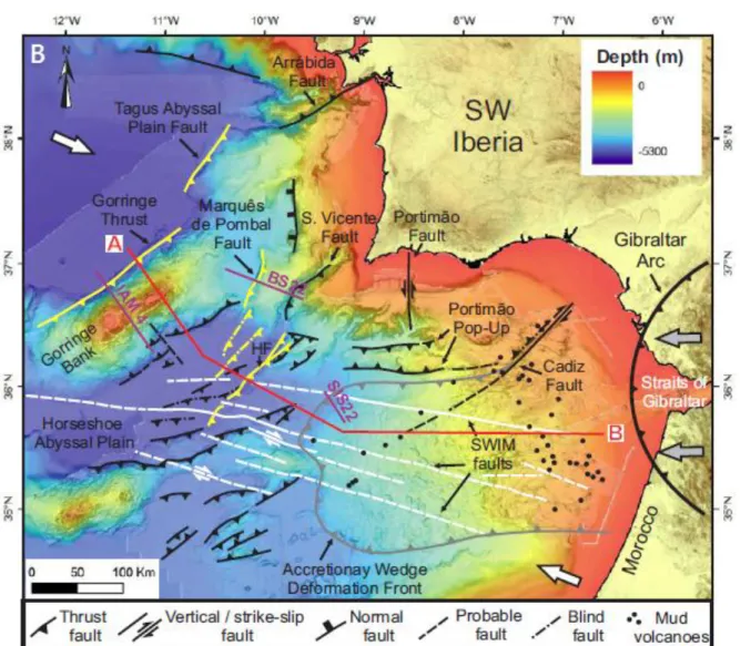
The epicenter location of the earthquakes 1755 and 1969 were somewhere southwest close to the Iberian Peninsula. This area is called Southwest Iberian Margin (SWIM), and it is known for its complex tectonics and heterogeneous morphology. It is composed of various seamounts like the Gorringe Bank, high ridges, low depressions, valleys and an accretionary wedge (see Fig. 1.4). The SWIM is located at the eastern end of the Nubia-Eurasia plate boundary offshore Southwest Iberia and Northwest Morocco. It is as an approximately 1000x400km stretch where the plate boundary is diffuse (Satori et al., 1994; Tortella et al., 1997 and Hayward et al., 1999). The area is characterized by a widespread active seismicity (Cunha et al., 2012).

In consideration of the 1755 earthquake location Johnston (1996) used scale comparison of isoseismal maps of the 28th _{February 1969 event and suggested the Gorringe Bank, a seamount located about 200}

km southwest of Cape St. Vincent as possible candidate source. Baptista et al. (1998b) used hydrodynamic modelling and backward ray tracing to investigate on the source of the 1755 event suggesting a source located closer to the continent. Further investigation revealed several tectonic structures with tsunamigenic potential (Zitellini et al., 1999, García et al., 2003, Terrinha et al., 2003, Gutscher et al., 2002). Some authors suggest to consider multiple rupture scenarios (Zitellini et al., 1999, 2001; Gracía et al., 2003; Ribeiro et al., 2006; Terrinha et al., 2003, 2009) and Matias et al. (2013) suggest for multiple fault rupture events reoccurrence rates of 700 – 3500 yr or less and states that the proximity of the faults should be taken into account.

To better understand the morphology and kinematics of the crust in the SWIM (Sartori et al., 1994, Zitellini et al., 2001, Gutscher et al. 2003, Terrinha et al. 2003, Zitellini et al., 2009) various campaigns have been undertaken using multi-channel reflection seismic, refraction seismic, multibeam swath Bathymetry, and seismic tomography (e.g. ARRIFANO 1992, BIGSETS 1998, SISMAR 2001, SWIM 2009, NEAREST 2010). The analysis and interpretation of this data highlighted several tectonic structures. In the SWIM several considerable NE-SW trending and southeast dipping thrust faults (Zitellini et al., 2009, Matias et al., 2013) could be identified, namely: Gorringe Bank fault, Marques de Pombal fault, São Vincente fault, Horseshoe fault, Tagus Abyssal Plain fault, Coral Patch Ridge, Seine Hills faults, (Hayward et al., 1999; Zitellini et al., 2001; Terrinha et al., 2003; Grácia et al., 2003; Zitellini et al., 2004; Terrinha et al., 2009, Loriente et al., 2013) (see Fig. 1.4). Recently Martínez-Loriente et al. (2014) propose the Horseshoe Abyssal plain thrust fault located close to the Horseshoe fault. These thrust faults are intersected by large WNW-ESE trending dextral strike-slip faults called SWIM faults separated in Lineaments North and South (Zitellini et al., 2009). Zitellini et al. (2009) stated the SWIM faults may be in transition from a diffuse to discrete transform plate boundary setting but this theory was later refuted by Cunha et al. (2012). These faults nevertheless prove the recent dextral strike-slip movement (Rosas et al., 2009). In the eastern most part of the Gulf of Cadiz Gutscher et al. (2002) believe to have identified an active subduction dipping eastwards underneath the Gibraltar Arc

earthquakes but folding and faulting of young sediments at the Cadiz accretionary wedge and independent movement of the Alboran block causes controversy scientific discussion (e.g. Matias et al., 2013, Duarte et al., 2013). The slab roll back causes extension in the Alboran Sea and is responsible for the westward migration of the Gibraltar Arc. Duarte et al. (2013) states that the Alboran block moves distinctly at velocities of 3-6 mm yr-1_{, higher than the Africa Eurasia convergence (4 mm yr}-1_{) and}

additionally induces compressive stresses to the SWIM. Duarte et al. (2013) suggest that both mechanism may lead to passive margin reactivation as the Gibraltar Arc propagates westwards although the migration velocity has been proven to slow down (Gutscher et al., 2012).

However, oblique NW-SE to WNW-ESE striking occurs according to kinematic plate models based on GPS data at rates of 4.5-6 mm yr-1 _{(Sella et al., 2002; McClusky et al., 2003; Fernandes et al., 2003;}

Nocquet & Calais et al., 2004). Rosas et al. (2012) used analogue and numerical modelling techniques obtaining coherent results and similar morphological features in the corner zone between the strike-slip SWIM faults and the Horseshoe fault. Other recent studies confirm the complexity of the SWIMs interior and state incipient and relic subduction and active thrust faults (Duarte et al., 2013, Monna et al., 2015). The dynamic processes of the SWIM have been eagerly discussed in literature and two main acting motors have been identified as NW-SE convergence between Africa and Eurasia and westward Gibraltar Arc migration. The importance and future development of each of the contributors is not doubtlessly clarified stressing the need of further investigations. Successive research revealed stepwise more parts of the SWIM puzzle classifying the area as a major source of tsunamigenic earthquakes. Systematized tsunami hazard assessment is required to launch adequate mitigation measures. Especially the tectonic uncertainties confirm the need evacuation measures based on tsunami hazard assessments and an operational tsunami warning system. Further west of the SWIM the Nubia-Eurasia plate boundary is defined as strike-slip fault linked to the Mid-Atlantic Ridge at the Azores triple junction. The eastern segment is called Gloria-Fault a 400km long fault with right lateral slip (Gonzales et al., 1996) and the part at Azores Islands is called the Terceira Ridge. The Terceira Ridge with high moderate seismicity is linked to the Mid-Atlantic Ridge at the Azores Triple Junction (see Fig. 1.3). Common mechanism in the area are normal and transform faulting (Tortella et al. 1997). At the Gloria fault between 24° W and 19° W several large strike-slip events took places in the 20th _{century (eg. Gutenberg and Richter, 1949;}

Lynnes and Ruff, 1975 and Grimson and Chen, 1986). The events on 25th _{November 1941 and 26}th _May

1975 triggered small tsunamis with maximum amplitudes about 0.45m which were registered in Casablanca (Baptista and Miranda, 2009).

Figure 1.4 A: ATJ – Azores triple junction; AGFZ Azores-Gibraltar fracture zone B: Tectonic map of southwest Iberian Margin (SWIM). Grey arrows show Gibraltar Arc westward movement; white arrows

show Africa-Eurasia WNW-ESE convergence. Modified from Duarte et al. (2013)

Concluding, the Portuguese coast is prone to tsunami hazards by local (SWIM) and regional (Gloria fault) source areas. In both areas considerable earthquakes took place and some of them triggered tsunamis. The SWIM is not fully understood and composed of complex tectonic setting. This source area is of specific interest as it triggered the 1755 tsunami and due to the closeness to the Portuguese, Spanish and Moroccan coastlines. Both source areas must be considered when applying the DTHA in study areas located in Portugal, Spain or Morocco.

The earthquake scenarios used to simulate the tsunami impact scenarios in Sines are based on geological evidences. For this thesis the Maximum Credible Earthquake (MCE) and their typical fault (TF) (Miranda et al., 2008; Omira et al., 2009) has been used to produce the tsunami scenarios. This DTHA approach uses the SWIM and the Gloria as seismogenic source areas. Five TFs and their MCE scenarios have been considered to calculate the tsunami scenarios namely: the Gloria Fault (GF), the Cadiz Wedge Fault (CWF), the Gorringe Bank Fault (GBF), the Horseshoe Fault (HSF) and the Marques Pombal Fault (MPF). Additionally a composite rupture model of HSF and MPF (HSMPF) has been built as suggested by (Ribeiro et al., 2006).

2. Methodology

Tsunami hazard assessment is done using two different methodologies: Deterministic Tsunami Hazard Assessment (DTHA) and Probabilistic Tsunami Hazard Assessment (PTHA). This master thesis applies the DTHA approach.

The DTHA method consists of considering certain tsunami events, commonly the most credible earthquake (MCE) scenarios. It provides a description as precise as possible of the effects of large tsunamis that may be triggered by known tectonic and geological processes.

A tsunami hazard scenario corresponds to an event generated by a single or in some cases from multiple sources of fixed dimensions and location, usually corresponding to characteristic earthquakes or to the MCE derived from geological constrains. The chosen scenarios are then modelled numerically and their impact is studied in a specific study area. The methodology is used by a broad scientific community to establish tsunami mitigation measures and for coastal engineering purposes. For that this approach is a valuable tool for coastal disaster management.

2.1. Preparation of the tsunami simulation

For the determination of the single scenarios for DTHA and computation of tsunami propagation and impact for each scenario the benchmarked numerical code NSWING (Non-linear Shallow Water Model with Nested Grids) (Miranda et al., 2014) has been employed.

To model a tsunami numerically several information and data is necessary. The life of a tsunami may be divided in three stages, namely: Generation, Propagation and Inundation, and the same applies to tsunami numerical simulations. The analysis begins in identifying the tsunami source areas and gathering data of the typical faults (TFs) (c.f. paragraph 1.2). These parameters are then used to calculate initial sea surface elevation that constitutes the initial condition to initiate the numerical model. The study area needs to be re-built as a Digital Elevation Model (DEM) describing the bathymetric and topographic features. To better describe the coastal areas high resolution DEMs are needed close to the coast. Depending on the spatial extent from the tsunami source to the study area it is necessary employ a system of coupled nested grids to achieve an adequate resolution in the study area. In this paragraph these stages are described to comprehensively explain the proceeding used in this thesis.

The following steps are carried to launch the NSWING model: (i) Computation of the initial condition, (ii) Preparation of the DEM covering the oceanic path between the source area and the study area, (iii)

Implementation the DEM in a system of nested grids, (iv) Chose the physical quantities to describe the tsunami impact in the study area: run up, flow depth, maximum inundation distance, and launch the simulation.

(i) Computation of the initial condition: First it is necessary to establish the earthquake scenario upon

given fault parameters that will generate the tsunami. By knowing the tsunamigenic earthquake source areas and its TFs (Miranda et al., 2008 and Omira et al. 2009) that may affect the study area. It is important to study all possible sources and to use the parameters from the most recent published papers. The initial condition is then computed using the model presented by Okada (1985) embedded in Mirone suite (Luis, 2007). The known fault is drawn upon the parent grid. In this thesis the half minute North Atlantic grid (GEBCO, 2014) has been interpolated to 640m resolution for the parent grid called Layer01. The parent grids extent are from 12.924° W to -5.735° W and from 33.982° N to 39.230 N. This grid embraces all tsunamigenic source areas, the open ocean and the study area. The output of the initial condition is also a finite grid file with the same extensions as the parent grid. After computing the initial conditions for all (TFs) they are stored in a folder, from where the NSWING model is launched later. The theoretical background to model the initial condition is given qualitative manner in paragraph 2.2.

(ii) Building the DEM: In a second step the DEM of the study area, the city and port of Sines has

been built using GIS tools, namely ArcGIS and QGIS. A number of different data sets containing bathymetric and topographic information have been combined in order to obtain a maximum of detail in the study area. The different data sets used are: a set of high resolution LIDAR data set

2012), and a nautical chart (Instituto Hidrográfico de Portugal, 2010). Additionally GPS-RTK (Global Positioning System – Real Time Kinetic) has been applied in areas with missing information. A final resolution of 10 m could be produced and represents the study area properly. Main geological features such as rocky outcrops could be identified in the resulting DEM. A short theoretical introduction on building DEMs for tsunami modelling purposes is presented in paragraph 2.3.

(iii) Preparations of the nested grids and implementation of the DEM: To guarantee smooth propagation in the model and numerical stability a system of coupled nested grids has been applied and Courant-Friedrichs-Lewy condition (CFL) must be satisfied. The CFL condition is explained in paragraph 2.4. The resolution of the parent grid is 640m and the resolution of the DEM is 10m. In this step, 2 intermediate girds are produced to reduce the resolution to the scale of 10m in the DEM. A refinement factor of 4 has been applied to achieve the two grids called Layer21 and Layer31 with 160m and 40m respectively. To get smooth propagation of the tsunami when passing from one Layer to the next, the corresponding geographically smaller layers haven been nested using the TINTOL tool embedded in Mirone suite (Luis, 2007). This tool allows to obtain the correct nesting information (correct corner nodes and coordinates) upon the applied refinement factor. This information is than used to produce the higher resolute layer apart from the coarser layer. In the last step the DEM is implemented in Layer31 and nesting information for the Layer41 is produced. This information is than applied on the DEM to get the correct corner nodes and the resulting Layer41. Layer01 to Layer41 are stored together with the initial condition in the folder together with the initial condition. The prepared layers for the nested grids are shown in figure 2.1.

Figure 2.1 Schematic outline of the 4 Layer prepared for NSWING; Layer 41 contains the DEM.

(iv) Definition and launching the tsunami simulation: The NSWING operational files and the files described from (i) to (iii) are sufficient if prepared correctly to launch a tsunami simulation. To do this an executable batch file must be edited, so that NSWING can use the prior prepared files.

this study we additionally prepared a list in format DAT with geographical coordinates corresponding to the positions of the virtual tide gauges. NSWING reads this file and stores the free surface elevation in this point for a chosen time step. This way waveforms can be analysed and compared with existing records. The computation tsunami propagation and inundation are described in paragraph 2.4 and 2.5 respectively.

With the DTHA approach physical quantities such as wave height, flow depth, drawback, inundation extent or velocities can be approximated. These quantities serve to draw scenario maps, develop vulnerability studies and evacuation measurements. Maximum current speed is also an important parameter that can be mapped if the vulnerability of buildings or coastal structures is in focus of the study. Tsunami travel time maps show the first arrivals of the waves in the study area. Virtual tide gauges can be placed to analyse the waveforms arriving at the test site. Information such as polarity, period, maximum wave height at the tide gauges and attenuation time can be obtained. As the tide regime in the Atlantic is strong, i. e. there is a significant difference (of the order of meters) between high tide and low tide, the scenarios must include this effect. An aggregate scenario can be produced plotting the MWH and the MFD in each cell considering the contribution of the individual scenarios (Tinti et al., 2011).

The final results are presented in integrated hazard maps for all the considered and the aggregate scenario. The integrated hazard maps have been produced using GIS tools. Each integrated hazard map consists of MWH, MFD, MRU and MDB of the corresponding scenario. The static effect of tides is analysed for three different tidal stages mean lower low water (MLLW), mean sea level (MSL), and mean higher high water (MHHW). Further the contribution of each scenario to the aggregate tsunami impact at MSL condition has been calculated. The analysis of the waveforms produced at chosen virtual tide gauges provide information such as, arrival time, period, the biggest wave and attenuation time.

2.2. Generation of tsunamis in the source area

Tsunami are triggered by submarine earthquakes, landslides, volcanic eruptions or meteorite impacts. As stated earlier this thesis focuses on studying the tsunami hazard caused by earthquakes. They occur at or near to tectonic faults for example along plate boundaries. Three types of faults can be distinguished: strike-slip or transform faults, normal faults and thrust or invers faults. The movement along pure strike-slip faults is horizontally and usually do not cause tsunamis. In some cases rupture mechanism along these faults may also have a vertical component and have the potential to trigger a tsunami. Normal and inverse faults cause vertical seabed motion and they are capable to lift or lower the water column above triggering the motion at the sea surface. Inverse faults may have contributions of horizontal components.

The initial sea surface deformation is computed using the analytical formulae, after Mansinha & Smylie (1971) synthetized in Okada (1985). They represent the displacement field on the surface of an elastic half-space, when a dislocation of given direction and size is introduced at a given epicentral depth. The deformation is then transferred to the free surface assuming that the water layer above is considered as incompressible layer and the seabed deformation is transferred directly to the free surface of the ocean (Kajiura, 1970).

To compute the seabed deformation one needs information on the earthquake mechanism: fault plane parameters, magnitude and distribution of deformation along the fault plane.

Figure 2.2 Definition of an individual seismogenic source. (Istituto Nazionale di Geofisica e Vulcanologia, 2015)

The fault plane parameters are the length, L, the width, W, the slip – dislocation along the fault plane and the angles, strike, dip, rake & depth. Length and Width give the extensions of the fault plane. Strike, dip and rake are given in angular units. The strike is the angle relative to the north on a horizontal plane and describes the trending of the fault. The dip measures the inclination from the planar horizontal surface. And the rake gives the direction of the movement along the fault plane during a rupture in relation to the strike. The distances of the movement along the rake is given by the slip and is measured in meters. In figure 2.2 the described fault parameters are represented. Upon these variables the initial tsunami condition is calculated employing Okadas (1985) model and set to the sea surface to initiate propagation.

These model has some limitations as the rupture area is simplified to a rectangle and the rupture process is considered to instantaneous. Dutykh (2008) and Dutykh & Dias (2007) showed that this model is not appropriate tsunami earthquakes with slower rupture mechanism. However, in this study the application of the model is justified as it has been used for medium sized thrust faults and an instantaneous rupture can be assumed (Omira, 2010).

The seismic moment (Aki, 1972) is related to shear modulus 𝜇, the rupture area 𝐴 and the slip 𝐷

𝑀₀= 𝜇𝐴𝐷 (2.1)

Where 𝜇 is the shear modulus in (Pa), 𝐴 is the rupture area (m²) and 𝐷 is the mean net displacement on 𝐴 in (m).

However, important to state is that the seismic moment depends on the three factors. But only two of them may have direct influence on tsunami generation. The slip is the movement that describes the dislocation along the fault plane. Greater slip values produce greater amplitudes. And greater areas of the fault plane produce higher periods. The shear modulus 𝜇, thus is a property of the crust in the region and has no impact on the tsunami but on the resulting seismic moment 𝑀₀ and the moment magnitude, 𝑀_𝑤.

The moment magnitude serves to quantify the earthquakes strength. It was derived by Kanamori (1977) and is linked with the scalar seismic moment, 𝑀0. This scale has the big advantage that it does not

𝑀_𝑤=2

3log10(𝑀0) − 10.73 (2.2)

Table 3.1 in paragraph 3 summarizes all used fault parameters to calculate the initial conditions for the in paragraph 1.2 presented tsunami scenarios. The initial conditions for all considered tsunami scenarios have been computed in Mirone suite (Luis, 2007) that employs Okadas (1985) model.

2.3. Digital Elevation Model

In order to represent in sufficient quality the study area digital data of bathymetric and topographic features and/or charts are combined. The DEM is built in a Geographic Information System and the final output is a simple grid dataset where each cell has a single numerical elevation value. The resolution of the resulting DEM defines quality of the entire numerical tsunami model Tinti et al. (2011).

Tsunami propagation close to the coast and on land is critically dependent on the small scale effects; so, the DEM (digital elevation model) must be able to represent the most significant coastal features and the shoreline accurately. The DEM, representing the bare earth, was produced including: (i) the tsunami source area and the test site areas along the coast (ii) good horizontal resolution in the test areas in order to assure a full description of local effects (iii) continuity offshore-onshore in particular in respect to the vertical datum.

The information used to build the DEM may be vector or raster/grid data containing height or depth information. Vectorised datasets can be point, line or polygon information corresponding to different altitudes such as bathymetric or topographic contours of various charts or individual point measurements like individual gathered GPS data. On the other hand raster data contains equal sized squares as cells, where each cell represents its corresponding height information. Each dataset is given in a horizontal and vertical spatial reference system which is usually depending on the geographical location, spatial extent, and producing institution or end-user. For instance bathymetric charts for nautical purposes are commonly referenced to bathymetric zero and topographic data is usually set in relation to MSL. One must be aware to while DEM preparation to set all used data sets in the same reference system. These datasets are available in different qualities. A raster dataset with smaller cell size contains more detailed information as a dataset with bigger cell size. When combining two or more different datasets it is necessary to give preference to more accurate data to avoid ambiguities. The vectorised datasets may improve the final DEM especially if the available raster data is of poor quality. It is crucial to transform all used data in the same horizontal and spatial reference system. In a final step the resulting DEM should be evaluated and verified for instance by posterior GPS-measurements at specific control points. A 3-D representation also helps to avoid errors for example at dataset boundaries. The resulting DEM is presented in Fig. 2.3.

2.4. Tsunami Propagation & SWEs

The motion of any viscous fluid substances and gas is described by the Navier-Stokes Equations, which are based on the Newton’s second law conservation of momentum in three dimensions. In combination with the conservation of mass a system of four coupled nonlinear partial differential equations are formed for three velocity components and pressure. There is no complete analytical solution for these coupled system of equations. Approximations are introduced to obtain best possible solutions depending on the scale of the geophysical process to be studied. This thesis applies the shallow water model which neglects viscous forces and the depth integrated SWEs average vertical velocities and accelerations. Other models to simulate tsunamis are the Boussinesq long wave model and the complete fluid dynamic model. The SWEs remain the most used model used by computational codes. In the last two decades numerical codes like TUNAMI-N2 (Imamura 1995), MOST (Titov and Synolakis 1995; 1998), COMCOT (Liu et al., 1998) and more recently UNIBO-TSUFD (Tonini et al., 2011 & Tinti et al., 2013) have been developed to model with sufficient accuracy tsunami propagation and coastal impact. To start propagation all these codes apply the model presented by (Okada 1985) described in paragraph 2.2. However, all these models are based on the SWEs but use different numerical methods to solve them. This study uses the recently developed and benchmarked code NSWING (Non-linear Shallow Water Model with Nested Grids) (Miranda et al., 2014). NSWING has been benchmarked following the definitions presented by Synolakis (2006). It is entirely written in C and applies core parallelisation enhancing computational performance.

The equations that govern the motion of tsunamis are called Navier-Stokes Equations. They represent Newton’s conservation of momentum in three dimensions in a cartesian frame (𝑥,𝑦,𝑧) (2.3a, 2.3b and 2.3c). These three equations in combination with the equation of conservation of mass (2.3d) build a system of four coupled non-linear partial differential equations.

𝑥: 𝜌 (𝑑𝑢 𝑑𝑡+ 𝑓∗𝑤 − 𝑓𝑣) = − 𝜕𝑝 𝜕𝑥+ 𝜕𝜏𝑥𝑥 𝜕𝑥 + 𝜕𝜏𝑥𝑦 𝜕𝑦 + 𝜕𝜏𝑥𝑧 𝜕𝑧 (2.3a) 𝑦: 𝜌 (𝑑𝑣 𝑑𝑡+ 𝑓𝑢) = − 𝜕𝑝 𝜕𝑦+ 𝜕𝜏𝑥𝑦 𝜕𝑥 + 𝜕𝜏𝑦𝑦 𝜕𝑦 + 𝜕𝜏𝑦𝑧 𝜕𝑧 (2.3b) 𝑧: 𝜌 (𝑑𝑤 𝑑𝑡 − 𝑓∗𝑢) = − 𝜕𝑝 𝜕𝑧− 𝜌𝑔 + 𝜕𝜏𝑥𝑧 𝜕𝑥 + 𝜕𝜏𝑦𝑧 𝜕𝑦 + 𝜕𝜏𝑧𝑧 𝜕𝑧 (2.3c) 𝜕𝜌 𝜕𝑡+ 𝜕 𝜕𝑥(𝜌𝑢) + 𝜕 𝜕𝑦(𝜌𝑣) + 𝜕 𝜕𝑧(𝜌𝑤) = 0 (2.3d)

where 𝑥-, 𝑦- and 𝑧- axes are the coordinates in directions eastward, northward and upward respectively. The variables, 𝑢, 𝑣 and 𝑤 represent the velocity components in 𝑥, 𝑦 and 𝑧 directions, 𝑓 = 2𝛺 sin 𝜑 is the Coriolis parameter and 𝜑 is the latitude, 𝑓_∗= 2𝛺 cos 𝜑 is the reciprocal Coriolis parameter (which is neglected for the most geophysical approximations), where 𝛺 is the rotation rate of the earth, 𝜌 is the density, 𝑝 is the pressure, 𝑔 is the gravitational acceleration and the 𝜏 terms represent normal and shear stresses because of friction.

To solve these equations appropriate approximations are used depending on the scale of the geophysical motion to be studied. The considered approximations are applied to the Navier-Stokes equations to reduce them to the SWEs. To obtain the SWEs viscous stresses and any flow gradients in vertical direction are eliminated (Synolakis, 2006) which is considered as a valid approximation for long waves if ℎ ≤₂₅𝜆 (Intergovernmental Oceanographic Commission, 2013) is satisfied. The water body is assumed to be incompressible. The SWEs are derived by a depth average integration from the ocean bottom to the free surface and it is assumed that pressure distribution is hydrostatic everywhere. This allows to introduce the variable 𝜂 the free surface elevation through the hydrostatic approximation for the pressure, 𝑝 = 𝜌𝑔(𝑑 + 𝜂), where 𝑑 is the water depth. This assumption is valid and considered to deliver results with sufficient accuracy as tsunamis are considered as long waves propagating in shallow water as stated in the paragraph 1.2. The shallow water model calculates the evolution of the water surface