Detection of chemical species in Titan's atmosphere using high-resolution spectroscopy

UNIVERSIDADE DE LISBOA

FACULDADE DE CIÊNCIAS

DEPARTAMENTO FÍSICA

Detection of Chemical Species in Titan’s Atmosphere using

High-Resolution Spectroscopy

José Luís Fernandes Ribeiro

Mestrado em Física

Especialização em Astrofísica e Cosmologia

Dissertação orientada por:

Doutor Pedro Machado

Acknowledgments

This master’s thesis would not be possible without the support of my parents, Maria de F´atima Pereira Fernandes Ribeiro and Lu´ıs Carlos Pereira Ribeiro, who I would like to thank for believing in me, encouraging me and allowing me to embark on this journey of knowledge and discovery. They made the person that I am today.

I would like to thank all my friends and colleagues who accompanied me all these years for the great moments and new experiences that happened trough these years of university. They contributed a lot to my life and for that I am truly grateful. I just hope that I contributed to theirs as well.

I also would like to thank John Pritchard from ESO Operations Support for helping me getting the EsoReflex UVES pipeline working on my computer, without him we would probably wouldn’t have the Titan spectra reduced by now. And I also like to thank Doctor Santiago P´erez-Hoyos for his availability to teach our planetary sciences group how to use the NEMESIS Radiative Transfer model and Doctor Th´er`ese Encrenaz for providing the ISO Saturn and Jupiter data.

I would like to give a special thank you to Jo˜ao Dias and Constan¸ca Freire, for their support and help during this work.

Lastly, and surely not the least, I would like to thank my supervisor Pedro Machado for showing me how to be a scientist and how to do scientific work. And also for opening so many doors for me even though I am just now finishing my master’s degree. Thanks to him, my dream of exploring new worlds in our Universe is becoming a reality.

Resumo

O nosso Sistema Solar ´e muito diverso no tipo de planetas que cont´em. Planetas tel´uricos, que s˜ao principalmente constitu´ıdos por silicatos ou metais, gigantes gasosos, que s˜ao constitu´ıdos principalmente por hidrog´enio e h´elio, e gigantes gelados, onde ´agua, metano e amon´ıaco pre-dominam. Tal como as suas propriedades, as suas atmosferas tamb´em s˜ao distintas. No caso dos corpos rochosos, apenas quatro possuem uma atmosfera densa, Merc´urio, V´enus, Terra e, um dos objectos de observa¸c˜ao deste trabalho, Tit˜a.

Tit˜a ´e o ´unico corpo para al´em da Terra que possui um fluido est´avel na sua superf´ıcie. A sua atmosfera ´e constitu´ıda principalmente por azoto, metano, algum hidrog´enio e v´arios hidrocarbonetos. Tal como a da Terra, a atmosfera de Tit˜a est´a bem estruturada em troposfera, estratosfera, mesosfera e termosfera, sendo que a atmosfera ´e mais extensa do que a da Terra chegando a ter alturas de escala entre os 15 e os 50 km, pois Tit˜a tem uma for¸ca grav´ıtica mais baixa. Tit˜a tamb´em possui ventos em superota¸c˜ao, devido a ter um per´ıodo de rota¸c˜ao longo e s´ıncrono com o de transla¸c˜ao, e sofre de efeitos sazonais devido `a inclina¸c˜ao da sua ´orbita, que coincide com a inclina¸c˜ao da ´orbita de Saturno. Em m´edia, o seu lado diurno ´e mais frio que o seu lado nocturno. No p´olo onde ´e Inverno, na estratosfera baixa, as temperaturas chegam a ser 25 K mais baixas que o equador, no entanto a estratopausa ´e cerca de 20 K mais quente

Saturno, caracterizado pelo seu grande sistema de an´eis, possui uma atmosfera que ´e prin-cipalmente constitu´ıda por h´elio, seguindo-se metano, amon´ıaco e outros hidrocarbonetos e mol´eculas compostas por hidog´enio, f´osforo, carbono ou oxig´enio. Possui uma tropopausa bem definida perto dos 80 mbar, que separa uma estratosfera estavel em que a temperatura aumenta com a altitude de uma tropoesfera em que a temperatura aumenta com a profundidade. Devido `

a inclina¸c˜ao do seu plano de rota¸c˜ao sofre de efeitos sazonais tal como Tit˜a. Exitem gradientes de temperatura que diminuem com o aumento de press˜ao, chegando a ser de 40 K na estratosfera e 10 K na troposfera dos p´olos. Al´em disso o aspecto visual de Saturno tamb´em muda, metano, que aprece com tons de azul, ´e facilmente destru´ıdo pela radia¸c˜ao solar. O hemisf´erio que estiver mais sujeito `a radia¸c˜ao solar (Ver˜ao) ter´a menos metano e ter´a mais uma cor castanha enquanto que o outro (Inverno) ser´a mais azulado. Quanto `a dinˆamica, a atmosfera tem uma circula¸c˜ao zonal leste, com v´arios v´ortices e nuvens. Sendo o mais peculiar o v´ortice hexagonal no p´olo norte de Saturno.

J´upiter ´e o planeta mais massivo do Sistema Solar, tendo mais do dobro da massa de todos os outros planetas combinados. A sua composi¸c˜ao ´e a que se aproxima mais a uma composi¸c˜ao proto-estelar de todos os gigantes gasosos, mas abundˆancia de elementos pesados como o carbono ou o nitrog´enio ´e trˆes a cinco vezes maior do que seria esperado numa proto-estrela. Indicando que J´upiter formou-se com planetesimais gelados e adquiriu massa suficiente para atrair grandes quantidade de g´as da nebulosa. A sua atmosfera, `a semelhan¸ca da de Saturno, ´e maioritaria-mente composta por h´elio, seguindo-se metano, amon´ıaco, hidrocarbonetos, alguns gases nobres e mol´eculas compostas por hidrog´enio, f´osforo ou oxig´enio. Abaixo do n´ıvel de 1 bar de press˜ao, a troposfera de J´upiter ´e caracterizada por v´arias nuvens dominadas por v´arias esp´ecies qu´ımicas diferentes. Perto dos 5 bar existe forte evidˆencias de nuvens de ´agua. Para n´ıveis acima dos 300 mbar de press˜ao encontra-se a estratosfera, onde neblinas combinam com nuvens de amon´ıaco que est˜ao contaminadas com hidrocarbonetos e possivelmente o al´otropo de f´osforo que poder´a dar a cor vermelha em certas zona desta camada. A press˜oes abaixo de 1 µbar encontra-se a termosfera onde ocorre desassocia¸c˜ao de mol´eculas por part´ıculas carregadas e auroras

gi-gantescas ocorrem nos p´olos. Dinamicamente, existem dois tipos de teorias para a atmosfera de J´upiter: modelos superficiais, que dizem que os jactos s˜ao conduzidos por turbulˆencias em pequena escala, onde a produ¸c˜ao de jactos ´e devido `a combina¸c˜ao de penas estruturas para formar estruturas maiores, no entanto estes jactos s˜ao inst´aveis, e modelos profundos, baseados na rota¸c˜ao organizada de s´eries de cilindros paralelos ao eixo de rota¸c˜ao, que conseguem explicar bem o jacto pr´ogrado no equador de J´upiter, mas produz um n´umero muito pequeno de jactos largos.

Os dados de Tit˜a e parte dos dados de Saturno foram adquiridos atrav´es do espectr´ografo UVES do VLT. UVES ´e um espectr´ografo que esta desenhado para operar com alta eficiˆencia dos 300 nm at´e aos 1100 nm. Possui dois bra¸cos (vermelho e azul) que podem ser operados em separado ou ambos ao mesmo tempo. O bra¸co vermelho cobre a radia¸c˜ao dos 420 nm at´e aso 1100 nm e est´a equipado com um mosaico CCD feito com um chip EEV e um chip MIT. O bra¸co azul cobre a luz dos 300 nm at´e aos 500 nm e apenas tem um CCD EEV.

Os restantes dados de Saturno e os dados de J´upiter foram fornecidos pela Doutora Th´er`ese Encrenaz. Estes dados s˜ao espectros obtidos pelo ISO, o primeiro observat´orio de infra-vermelhos orbitante. Estava equipado com uma cˆamera de infra-vermelhos, com dois detectores , o SW e o LW, que cobria a radia¸c˜ao dos 2.5 aos 17 micr´ometros, o foto-polarimetro ISOPHOT (2.5 aos 240 micr´ometros) e dois espectr´ometros, o SWS (2.4 at´e 45 micr´ometros),de onde provieram os dados, e o LWS (45 a 196.8 micr´ometros).

A redu¸c˜ao dos dados de Tit˜a foi feita com o recurso `a pipeline do UVES do EsoRelfex. Esta pipeline faz a calibra¸c˜ao em bias, flat e dark como tamb´em faz a calibra¸c˜ao em comprimento de onda dos dados. Como esta pipeline ´e geral, para o caso de uma fonte extensa como Tit˜a foi necess´ario mudar o m´etodo de extrac¸c˜ao para ’2D’.

A redu¸c˜ao dos dados UVES de Saturno foi feita usando a pipeline de Espectroscopia de Alta-Resolu¸c˜ao do IA, que de maneira semelhante ao EsoReflex, faz as calibra¸c˜oes dos dados. Esta pipeline calcula os desvios de Doppler em cada ponto da imagem do alvo para medir a velocidade dos ventos, mas isso vai para al´em dos objectivos deste trabalho.

Para a detec¸c˜ao de mol´eculas em Tit˜a recorreu-se `as bases de dados de transi¸c˜oes molec-ulares HITRAN e ExoMol. Nelas procurou-se quais as mol´eculas que seriam poss´ıveis serem encontradas no espectro de Tit˜a dentro dos limites de comprimento de onda. Verificou-se que seria H2 , HD e H2O16

Para Tit˜a detectou-se v´arias poss´ıveis transi¸c˜oes de H2O16, H2 e HD como tamb´em uma

poss´ıvel transi¸c˜ao de C₃. At´e ser feita a calibra¸c˜ao em fluxo do espectro para se obter unidades f´ısicas, n˜ao se pode considerar todas as detec¸c˜oes como certas pois pode haver altera¸c˜oes na forma do espectro. No entanto, vindo-se a confirmar a detec¸c˜ao de C₃, ser´a ent˜ao confirmada a previs˜ao descrita na proposta de observa¸c˜ao.

Nos dados UVES de Saturno detectou-se a banda de CH4 nos 619 nm mas a calibra¸c˜ao ´e

fluxo destes dados n˜ao ser´a poss´ıvel, pois nenhuma estrela de calibra¸c˜ao foi observada durante as observa¸c˜oes. Detectou-se nos dados do ISO a emiss˜ao C4H2 nos 15.92 µm.

Por ´ultimo, em J´upiter detectou-se v´arias linhas de emiss˜ao de H+₃ entre 3.5 e 3.9 µm. Detecou-se a linha de absor¸c˜ao de CH₄ nos 2.6 µm e banda de emiss˜ao ν₃ de CH₄ nos 3.3 µm. Quanto a NH3 foram detectadas v´arias bandas de absor¸c˜ao entre os 9 µm e os 12 µm.

Palavras-chave:

Abstract

The basis behind the understanding the spectrum of radiation from an atmosphere is Ra-diative Transfer. It tells us how the shape, width and depth of each molecular transitional line are influenced by the conditions of the environment where these molecules inhabit and if there is surface on that planet.

This thesis reports on the use of various tools and instruments in order to determine the presence of chemical species in the atmospheres of various objects in our solar system

For the case of Titan, dedicated UVES observations were used and reduced with the EsoRe-flex UVES pipeline in order to detect multiple possible transitional lines of H2O, H2 and HD,

as well as a possible transitional line of C₃ which might confirm the predictions stated in the observations application [1].

For the case of Saturn, UVES observations were used as well as spectra from the ISO space telescope provided by Doctor Th´er`ese Encrenaz. The UVES data was reduced by the IA’s High-Resolution Spectroscopy pipeline and in it the 619 nm CH4 band was detected. In the ISO data

the C4H2 was detected.

For the case of Jupiter, ISO spectra provided by Doctor Th´er`ese Encrenaz were used. In the spectra, the 2.6 microns absorption and the ν3 emission band at 3.3 microns were detected

for CH4, multiple absorption bands at the 9 to 12 microns range were detected for NH3, and

multiple H+₃ emission lines were detected as well.

In the future, we intend to use the Saturn and Jupiter ISO data to retrace the steps from [2] and [3] in order to learn how to use the NEMESIS Radiative Transfer model [4] and apply it to the Titan data in order to obtain its temperature and pressure profile.

Keywords:

Contents

1.1.1 Titan’s Atmosphere . . . 1 1.1.2 Exploration of Titan . . . 9 1.2 Saturn . . . 10 1.2.1 Saturn’s Atmosphere . . . 10 1.2.2 Exploration of Saturn . . . 13 1.3 Jupiter . . . 15 1.3.1 Jupiter’s Atmosphere . . . 15 1.3.2 Exploration of Jupiter . . . 18

2 Methods and Tools 19 2.1 Radiative Transfer . . . 19

2.2 UVES - Ultraviolet and Visual Echelle Spectrograph . . . 21

2.3 ISO – The Infrared Space Observatory . . . 22

2.4 The IA’s High-Resolution Spectroscopy Pipeline . . . 23

2.5 EsoReflex: UVES pipeline . . . 24

2.6 HITRAN & ExoMol . . . 26

2.7 Flux Calibration . . . 26 3 Observations 29 3.1 Titan . . . 29 3.2 Saturn . . . 29 3.3 Jupiter . . . 30 4 Results 31 4.1 Titan . . . 31 4.1.1 H₂O . . . 31 4.1.2 H2 . . . 33 4.1.3 HD . . . 35 4.1.4 C₃ . . . 37

4.2 Saturn . . . 38 4.3 Jupiter . . . 40 5 Discussion 43 5.1 Titan . . . 43 5.2 Saturn . . . 45 5.3 Jupiter . . . 45 6 Conclusions 47 6.1 Future Work . . . 47 Bibliography 49 A NEMESIS - 53

List of Tables

1.1 Stratospheric composition of Titan . . . 2

1.2 Composition of Titan’s neutral atmosphere . . . 3

1.3 Composition of Saturn . . . 11

List of Figures

1.1 View of Titan . . . 1

1.2 The photochemestry of CH₄ in Titan’s Atmosphere . . . 4

1.3 The photochemestry of N2 in Titan’s Atmosphere . . . 5

1.4 Representative temperature profile for Titan’s atmosphere . . . 6

1.5 The thermal profile of Titan’s atmosphere [6] . . . 7

1.6 Cassini’s ’Last Dance’: A Final Portrait at Saturn . . . 10

1.7 Approximation of the latitudinal profile of the wind speeds in the Saturn’s atmo-sphere . . . 13

1.8 Vivid auroras in Jupiter’s atmosphere . . . 15

2.1 Photo of UVES at the Nasmyth B focus of UT2 of VLT . . . 21

2.2 The ISO satellite . . . 22

2.3 1D spectrum of Saturn . . . 23

2.4 Esoreflex enviroment . . . 24

2.5 Editing the parameters of the Spectrum Extraction actor for the case of Titan . 25 2.6 Selection of data to be processed using EsoReflex . . . 25

2.7 Absolute flux and HARPS measured flux of Piscium . . . 27

2.8 Response function of the instrument HARPS north . . . 27

2.9 Venus spectrum obtained by the HARPS north instrument with arbitrary units of intensity as function of wavelength (Left plot). Venus spectrum calibrated using the response function with absolute units of intensity as function of wavelength (Right plot) . . . 27

4.1 Output of HITRAN for H2O transition lines . . . 31

4.2 Telluric H2O absorption line at 3993.17 ˚A and Titan’s at 3993.37 ˚A . . . 32

4.3 Telluric H₂O absorption line at 4425.5 ˚A and Titan’s at 4425.8 ˚A . . . 32

4.4 Telluric H₂O absorption line at 4440.9 ˚A and Titan’s at 4441.2 ˚A . . . 33

4.5 Output of HITRAN for H₂ transition lines . . . 33

4.6 Telluric H₂ absorption line at 4539.3 ˚A and Titan’s at 4539.6 ˚A . . . 34

4.7 Telluric H2 absorption line at 4549.9 ˚A and Titan’s at 4550.2 ˚A . . . 34

4.8 Telluric H2 absorption line at 4596.2 ˚A and Titan’s at 4596.5 ˚A . . . 35

4.9 Output of HITRAN for HD transition lines . . . 35

4.10 Telluric HD absorption line at 4567.8 ˚A and Titan’s at 4568.1 ˚A . . . 36

4.11 Telluric HD absorption line at 4569.8 ˚A and Titan’s at 4570.1 ˚A . . . 36

4.12 Transmittance of C₃ . . . 37

4.14 Apparent telluric C₃ absorption line at 4042.0 ˚A and Titan’s at 4042.3 ˚A . . . . 38

4.15 Visible spectra of the gas giants . . . 38

4.16 Saturn’s 619 nm methane band . . . 39

4.17 C4H2 emission at 15.92 µm . . . . 39

4.18 H+₃ emission in the 3.5 to 3.9 microns region . . . 40

4.19 CH₄ absorption at 2.6 microns . . . 40

4.20 ν3 CH4 band emission at 3.3 microns . . . 41

4.21 NH₃ lines in the 9 to 12 microns region . . . 41

5.1 Telluric H₂O absorption line at 4427.4 ˚A and no Titan line at 4427.7 ˚A . . . 43

5.2 H2O transition lines . . . 44

5.3 Absence of C₃ telluric and Titan lines at 4050.6 ˚A and 4050.9 ˚A respectively . . 45

Chapter 1

Introduction

1.1

Titan - The largest moon of Saturn

Figure 1.1: View of Titan taken with the high resolution camera on board Cassini. Credits to NASA [5]

Titan is a quite peculiar celestial body. Besides being the largest of satellite of Saturn and the second largest of the Solar System, it is the only satellite in the Solar System to have a dense atmosphere [6]. Another striking feature of Titan is that is the only solar system body besides Earth to currently possess stable liquid on it’s surface [7].

1.1.1 Titan’s Atmosphere

Composition

Several molecules were detected with infrared spectroscopy (C2H6, CH3D, and C2H2). But

with the Voyager flyby there was a big leap in the number of chemical species detected. N₂, H₂, HCN, C3H8, C2H4, C3H4 (CH3C2H), C4H2, HC3N, C2N2 and CO2 were first identified and then

later confirmed by the ISO space telescope. H2O was detected by ISO and CO was detected

chemical species are in the table 1.1

Table 1.1: Stratospheric composition of Titan. Columns 4 and 5 define the vertical distribution of the components in the north polar region, from two pressure/altitude levels in the atmosphere; 0.1 hPa/250 km and 1.5 hPa/120 km * in the troposphere, * * in the stratosphere [6]

The Cassini-Huygens probe made a huge leap in our knowledge of the composition of the moon’s atmosphere. It was equipped with powerful remote sensing and in situ instruments that allowed the detection and measurement of chemical species and characterisation of aerosol particles. The Composite Infrared Spectrometer (CIRS) improved our understanding of small molecule chemistry and constrained the dynamics and seasonal changes thanks to temporal and spatial measurements of Titan’s stratosphere [7] as well as detecting propene for the first time(C3H6) [8] in the atmosphere of Titan. The Ultraviolet Imaging Spectrograph (UVIS)

pro-vided the composition and temperature information necessary to complete our understanding of Titan’s atmospheric structure by sensing the previously unexplored mesosphere. Additionally, the Gas Chromatograph and Mass Spectrometer (GCMS), the Ion and Neutral Mass Spec-trometer (INMS) and Cassini Plasma SpecSpec-trometer (CAPS) allowed us to measure regions of the atmosphere that cannot be accessed with remote sensing due to density. Numerous previ-ously undetected species have been identified in measurements obtained by the INMS in Titan’s thermosphere as well [7].

Cassini-Huygens and ground-based telescopes with abundances given in mole fractions. It shows how the mole fractions changed from the initial Voyager and ISO measurements (Table 1.1), covers a bigger altitude range than Table 1.1 and shows that several other molecules were identified (CH3C2H, C3H6, C6H6, HNC, CH3CN, C2H5CN, NH3).

Stratosphere Mesosphere Thermosphere

Formula Ground Based ISO/Herschel CIRS UVIS INMS (CSN)

H2 9.6 ± 2.4 × 10−4 3.9 ± 0.01 × 10−3 40_{Ar 1.1 ± 0.03 × 10}−5 C2H2 5.5 ± 0.5 × 10−6 2.97 × 10−6 5.9 ± 0.6 × 10−5 3.1 ± 1.1 × 10−4 C2H4 1.2 ± 0.3 × 10−7 1.2 × 10−7 1.6 ± 0.7 × 10−6 3.1 ± 1.1 × 10−4 C2H6 2.0 ± 0.8 × 10−5 7.3 × 10−6 7.3 ± 2.6 × 10−5 CH3C2H 1.2 ± 0.4 × 10−8 4.8 × 10−9 1.4 ± 0.9 × 10−4 C3H6 2.6 ± 1.6 × 10−9 2.3 ± 0.2 × 10−6 C3H8 6.2 ± 1.2 × 10−7 2.0 ± 1.0 × 10−7 4.5 × 10−7 < 4.8 × 10−5 C4H2 2.0 ± 0.5 × 10−9 1.12 × 10−9 7.6 ± 0.9 × 10−7 6.4 ± 2.7 × 10−5 C6H6 4.0 ± 3.0 × 10−10 2.2 × 10−10 2.3 ± 0.3 × 10−7 8.95 ± 0.44 × 10−7 HCN 5 × 10−7 3.0 ± 0.5 × 10−7 6.7 × 10−8 1.6 ± 0.7 × 10−5 HNC 4.9 ± 0.3 × 10−9 4.5 ± 1.2 × 10−9 HC3N 3 × 10−11 5.0 ± 3.5 × 10−10 2.8 × 10−10 2.4 ± 0.3 × 10−6 3.2 ± 0.7 × 10−5 CH3CN 8 × 10−9 < 1.1 × 10−7 3.1 ± 0.7 × 10−5 C2H5CN 2.8 × 10−10 C2N2 9 × 10−10 4.8 ± 0.8 × 10−5 NH3 < 1.9 × 10−10 < 1.3 × 10−9 2.99 ± 0.22 × 10−5 CO 5.1 ± 0.4 × 10−5 4.0 ± 5 × 10−5 4.7 ± 0.8 × 10−5 H2O 8 × 10−9/7 × 10−10 4.5 ± 1.5 × 10−10 < 3.42 × 10−6 CO2 2.0 ± 0.2 × 10−8 1.1 × 10−8 < 8.49 × 10−7

Table 1.2: Composition of Titan’s neutral atmosphere [7]

Titan was formed around the same time as Saturn, in a region of the solar system where the temperatures are low and icy materials such as NH₃ and CH₄ are abundant as clathrate hydrates. Nitrogen (the main component) was captured as NH₃ and in other non-N₂-bearing compounds as indicated by the measurements of the atmospheric composition and isotopic ratio of primordial noble gases by the Huygens probe. The actual nitrogen atmosphere results from the subsequent photolysis in a hot proto-atmosphere generated by the accreting Titan or possibly due to the impact-driven chemistry of NH3. However, ammonia is easily photodissociated into

N₂ and H₂ by sunlight. The nitrogen molecule is retained by Titan’s gravity but the molecular hydrogen escapes. Resulting in Titan building up a N2 atmosphere like the Earth’s from an

original secondary atmosphere that was rich in NH₃ [9]. In the case of CH₄, chemical reactions induced by sunlight build hydrocarbons such as ethane, acetylene, and propane that can form long molecular chains (polymers) that remain suspended in the atmosphere forming an aerosol haze layer while others will sink to coat Titan’s surface. In other words, photochemistry destroys methane irreversibly on Titan, so methane must be continually or periodically replenished on Titan. The most probably the source is geological source with a possible clathrate reservoir as storage in the interior of Titan [9].

The photochemistry of CH4 leads to the formation of significant quantities of the follow-ing components: C2H4, C2H2, C3H4, C2H6, C3H8, and C4H2, all of which are observed, and

additionally: CH₂, CH₃, C₂H, C₄H, C₆H₂ and C₈H₂, leading to chains of polymers (the poly-acetylenes C2nH2). Shown in Figure 1.2 [6].

Figure 1.2: The photochemestry of CH4 in Titan’s Atmosphere [6]

From the dissociation of N₂ by energetic magnetospheric electrons, we obtain the N+ ion, which itself dissociates CH4. This then leads to HCN, C2N2, and HC3N, all of which are

observed, and thence to the (HCN)n polymers, up to adenine, one of the four bases involved in

Structure

Figure 1.4: Representative temperature profile for Titan’s atmosphere, some of the major chemical processes, and the approximate altitude coverage of the instruments carried by Cassini-Huygens [7]

Similar to Earth’s, the vertical temperature structure in Titan’s atmosphere has a well-defined troposphere, stratosphere, mesosphere, and thermosphere. Titan’s atmosphere is more extended despite being colder than Earth’s, with scale heights of 15 to 50 km (compared to 5 to 8 km on Earth) due to Titan’s lower gravity. Due to efficient cooling by HCN rotational lines temperatures in the thermosphere are similar to those in the mesosphere, despite the significant EUV heating rates in the thermosphere [7].

The variability and complexixty of the thermal structure of the upper atmosphere surpasses expectations. On average the day side is colder than the night side [10, 11]. Temperature and latitude don’t appear to be correlated, which idicates that solar input does not control the temperature [7]. Additionally, the coldest temperatures are measured when Titan is out-side the magnetosphere while the highest temperatures are seen when Titan is inout-side Saturn’s magnetosphere, [10, 11].

Analyses of the Huygens Atmospheric Structure Instrument (HASI) data found that the planetary boundary layer (PBL) is located at 300 m [12], while analyses of dune spacing [13] and temperature measurements [14] found that the PBL is located at 2-3 km. However, Titan should have two PBLs as shown by the General Circulation Model (GCM) of Charnay and Lebonnois [15], a seasonal one located at 2 km and a diurnal one that reaches up to 800 m over the course of a day making it consistent with the Huygens’ measurement at 300 m that coincided with the mid-morning arrival of the Huygens Probe [7].

The thermal structure of the lower atmosphere was determined thanks to the results from the Voyager radio occultation, this includes the conditions at the surface: a pressure of 1.5±0.2 bar and a temperature of about 94 K. The temperature profiles are valid between the surface and the 10-hPa (10-mbar) pressure level, however, the profiles depend on the mean molecular mass

selected, but beyond that the inaccuracy inherent in the initial choice of conditions becomes too great. The IRIS infrared-spectrometer experiments provided complementary information about the thermal structure as well. Figure 1.5 shows the profile derived from the two experiments [6].

Figure 1.5: The thermal profile of Titan’s atmosphere [6]

The Voyager images have also shown that Titan is covered by a cloud layer opaque to visible radiation, that is yellowish-orange in colour. In addition, the images of the moons’s limb showed the presence of a haze layer at an altitude of about 300 km [6].

Dynamics

The winds in Titan’s atmosphere result primarily from solar forcing, which varies seasonally. Direct measurements of the wind speeds come from a few methods, each with limitations:

• Measurements from the Doppler Wind Experiment (DWE) carried by the Huygens probe - Provided measurements at one place and time from 145 km to the surface;

• Measuring Doppler shifts in the emission lines of atmospheric constituents - Has the ad-vantage of being possible from Earth, but provides limited spatial resolution;

• Cloud tracking - Used to measure wind speeds in planetary atmospheres, but the general paucity of clouds on Titan means that cloud tracking provides temporally and spatially limited wind speed measurements;

Indirect techniques have also been used to constrain the winds on Titan including stellar occul-tations and the use of the thermal wind equation to calculate wind speeds from temperature measurements. Wind speeds can also be constrained through evidence of aeolian processes such as dunes and wind-driven waves on the lakes and seas [7].

Cloud tracking measurements find wind speeds primarily eastward ranging from 0.5 to 10 m/s, although speeds up to 34 ± 13 m/s have been reported [16] in the troposphere. Titan

shows stratospheric superrotating winds (up to ∼ 200 m/s) higher in the atmosphere which then decrease in the upper stratosphere and lower mesosphere [17]. Taken together, the zonal wind speeds are very low (< 1 m/s) at the surface increasing to ∼ 40 m/s near 60 km where they begin decreasing until they reach a minimum (∼ 5 m/s) around 75 km before increasing again to 200 m/s near 200 km then decreasing to 60 m/s at higher altitudes (near 450 km) [7]. Averaged CIRS measurements from 2004 to 2006 (northern winter) by Achterberg et al. [17] showed that the stratospheric jet was centered between 30◦ N and 50◦ N at a pressure of 0.1 mbar and they also argue that although pre-Cassini temporal coverage is sparse, it is consistent with the presence of a strong jet in the winter hemisphere, which forms sometime in the fall and dissipates after spring equinox [7].

In the lower troposphere (up to ∼ 20 km) the meridional wind speeds have been estimated to be an average of 0.1 m/s northward above 1 km (peaking at 0.4 m/s) and southward below 1 km (peaking at 0.9 m/s) based on images taken by DISR [18].

Due to Titan’s slow rotation it is possible for global Hadley circulation to exist, with descend-ing motion near the winter pole and ascenddescend-ing motion in the summer hemisphere, to redistribute heat.Titan generally has one main cell (pole to pole), except near the equinoxes when there are two cells (equator to pole) as the circulation reverses which contrasts with Earth, where the strength of the Coriolis force limits the latitudinal extent of meridional circulation cells. The relatively small equator to pole temperature contrasts is the result of the single Hadley cell efficiently redistributing heat [7].

Another defining characteristics of Titan’s atmospheric circulation is the presence of super-rotating winds in the stratosphere including a strong jet near 0.1 mbar ( ∼ 300 km) in the winter hemisphere. Unlike Venus, that also has superrotating winds, Titan has a strong seasonal cycle that acts to prevent the generation of superrotating winds, which complicates the atmospheric dynamics [7].

Superrotation and zonal jets depend on the mean meridional circulation, which is determined by rotation rate, planetary radius, and solar heating, and is also related to the gas, haze, and cloud distributions due it is also being affected by radiative transport [7].

Seasonal Variation

Seasonal effects are important over a Titan year (29.5 Earth years) because of Saturn’s axial tilt of almost 27 ◦

Strong variations with latitude for stratospheric mixing ratios were shown by both Voyager IRIS and Cassini CIRS measurements as well as hydrocarbons and nitriles being more abundant at the winter pole than at lower latitudes or in the summer hemisphere. The strength of the latitudinal variation depends on the chemical lifetime of the species; short-lived species tend to exhibit stronger variations than long-lived species [7].

For most molecules at similar latitudes and seasons the observed abundances are consistent with no interannual variability indicated by the comparisons between Cassini CIRS and Voyager IRIS measurements [7].

The winter polar stratospheric temperature structure is reminiscent of Earth’s winter pole and consistent with subsidence. In the lower stratosphere, temperatures are at least 25 K colder than the equator [17]. However, higher in the atmosphere the stratopause is ∼ 20 K warmer than at the equator and is about two scale heights higher. Deeper in the atmosphere, temperature

decreases attributed to radiative cooling have been observed as the south pole moves into winter [7].

As a pole moves into summer there is a decrease in adiabatic heating and a decrease in temperature higher in the atmosphere due to the decreasing of the downwelling, while the deeper atmosphere warms as the photon flux increases. The gas mixing ratio enhancements also begin to dissipate [7].

1.1.2 Exploration of Titan

History of Titan’s Exploration

In 1908 Jos´e Comas Sol`a first suggested the possible existence of an atmosphere around Titan in his paper “Observations des satellites principaux de Jupiter et de Titan” from the existence of a limb-darkening effect [19].

In 1944 Gerard Kuiper discovered methane in Titan’s atmosphere, confirming the existence of an atmosphere [20].

During the 1970’s, Titan became the object of an intensive programme of observations from Earth, analyses of ground-based infrared spectra began to provide constraints on the tempera-ture structempera-ture [21] and composition of Titan’s Atmosphere [22]. However, it was concluded that CH₄ might be only a minor constituent and that other absorbers might be present [23], due to a detection of a greenhouse effect [21] coupled with detailed investigations of the spectral features of methane [22].

In 1971 the presence of N₂ was first suggested by Lewis based on the idea that Titan accreted NH₃ during formation, which later photolyzed to form N₂ [24].

In 1979 Pioneer 11 confirmed the presence of an aerosol absorber in the atmosphere of Titan [25] and provided a lower limit of 1.37 g/cm2 on Titan’s density [26].

In the 1980’s the flybys of the Voyager 1 and 2 confirmed that Titan has a substantial N₂ atmosphere [27], with a surface pressure 1.5 times that of Earth and a surface temperature of 94 K [14]. The infrared spectra taken by the Voyager spacecraft showed the presence of various organic molecules and gave us an initial idea of the complexity of the chemical and physical processes of this atmosphere [28].

Only in 2004, with the arrival of the Cassini-Huygens mission, was it possible to overcome Titan’s thick photochemical haze and observe directly for the first time the moon’s surface. Giving us, not only information about the atmosphere composition as well as how the atmosphere and the surface are correlated, the climate and how methane is resupplied to the atmosphere [7].

1.2

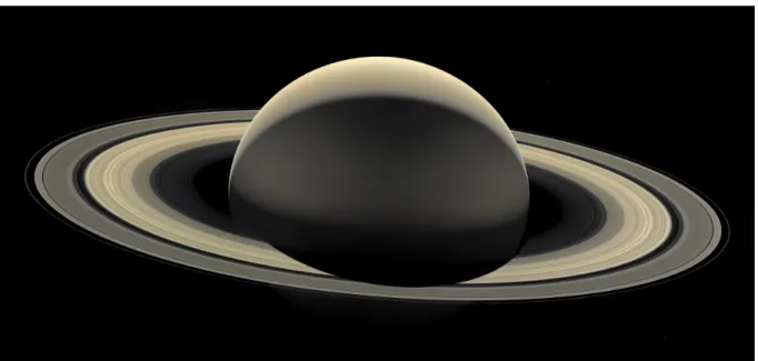
Saturn

Figure 1.6: Cassini’s ’Last Dance’: A Final Portrait at Saturn. Credits to: NASA / JPL-Caltech / SSI / Ian Regan

Saturn could be classified as one of the most unique planets in our solar system due to presence of its massive ring system. These rings, which are mainly composed of H2O ice, are

the biggest ring system of all the gas giants and appear to be significantly younger than the average age of the solar system, which indicates they may have been formed from tidal disruption of one or more captured satellites and not from a remnant of the solar nebula which became gravitationally bound to the planet [29].

1.2.1 Saturn’s Atmosphere

Composition

Saturn is mainly composed of hydrogen and helium and trace amounts of other elements, namely nitrogen, oxygen, carbon and phosphorous. Since this planet is less massive than Jupiter it indicates that it was able to attract a much smaller mass of H2and He from the nebula making

the mixing ratios of the heavier elements (X/H) to be correspondingly higher [29]. Table 1.3 shows the composition of Saturn with respective mole fractions and measurement techniques.

Gas Mole fraction Measurement technique

He 0.118 Voyager far-IR

NH3 ∼ 5 × 10−4 Ground-based microwave

H2S (3.4 pm 0.4) × 10−3 Ground-based 1.3, 2, 6, 21, and 70 cm

H2O 2.3 × 10−7 (upper troposphere) ISO 5 µm

CH4 (4.7 ± 0.2) × 10−3 CIRS far/mid-IR

CH3D (3.0 ± 0.2) × 10−7 CIRS mid-IR

PH3 (5.9 ± 0.2) × 10−6 at p > 500 mbar Cassini IR

AsH3 2.3 × 10−9 (troposphere) ISO 5 µm

GeH4 2.3 × 10−9 (troposphere) ISO 5 µm

CO 2.1 × 10−9 ISO 5 µm

C2H6 1.5 × 10−5 (0.5 - 1 mbar) Cassini mid-IR

C2H2 1.9 × 10−7 (2 mbar) Cassini mid-IR

C4H2 1 × 10−10 at p < 10 mbar ISO mid-IR

CH3C2H 7 × 10−10 at p < 10 mbar ISO mid-IR

CH3 (1.5 ± 7.5) × 1013 mol cm−2 ISO/SWS

CO2 3.4 × 10−10 at p < 10 mbar ISO mid-IR

HF < 8.0 × 10−12 Cassini far-IR

HCl < 6.7 × 10−11 Cassini far-IR

HBr < 1.3 × 10−10 Cassini far-IR

HI < 1.4 × 10−9 Cassini far-IR

Table 1.3: Composition of Saturn. Table excerpt taken from [29]

Structure

Temperatures from CIRS mapping observations show that Saturn has a well-defined tropopause at ∼ 80 mbar, separating a strongly statically stable stratosphere with temperatures increas-ing with altitude, from a troposphere with temperatures increasincreas-ing with depth. In the upper troposphere, the temperature gradient decreases with altitude down to approximately 400–500 mbar, where the gradient becomes nearly dry adiabatic. Stratospheric temperatures at 1 mbar show a strong pole to pole gradient, with the north (winter) pole being almost 40 K colder than the south (summer) pole. The hemispheric temperature asymmetry weakens with increasing pressure, with the the summer hemisphere being ∼ 10 K hotter than the winter hemisphere in the upper troposphere, and disappears at pressures greater than about 500 mbar where the tem-perature becomes nearly uniform with latitude. In addition to the large scale equator-to-pole temperature gradients, between ∼2–300 mbar there are temperature variations of 2–3 K on the scale of the zonal jets. Outside the equatorial region, the temperature gradients are correlated with the mean zonal winds, with warmer temperatures where the winds are cyclonic, and colder temperatures where the winds are anticyclonic. Temperatures in the equatorial region have been observed to oscillate with a period of ∼15 Earth years [30].

At the pressure range of 0.5 - 2 bar where temperatures range from 100 to 160 K, the clouds consist of NH3 ice. From ∼ 2.5 bar to 9.5 bar, where temperatures range from 185 - 270 K,

H₂O ice clouds become prominent. Intermixed in this layer in the pressure range 3 - 6 bar with temperatures of 290 - 235 K is a band of (NH4)HS ice. The lower layers contain a region

of water droplets with NH3 in aqueous solution, where pressures are between 10 - 20 bar and

Dynamics

Saturn has an atmospheric circulation that is dominated by zonal eastward flow [31].

The equatorial zone at latitudes below 20◦ shows a particularly active eastward flow having a maximum velocity close to 470 m/s but with periods when the velocity is 200 m/s slower [31].

The zonal flows are remarkably symmetrical about Saturn’s equator. Strong eastward flows (stronger than 100 m/s) are seen at 46◦ N and S and at about 60◦ N and S. Westward flows, are seen at 40◦, 55◦, and 70◦ N and S [31].

Strong hurricane-like cyclonic vortices are found within about 11◦ of both the north and south poles of Saturn. The warm eye of the vortex at the south pole has a diameter of 2000 km and is ringed by clouds towering 50 to 70 km above the polar clouds. The first jet to the south of the northern vortex at 75◦ N follows a hexagonal pattern around the planet. Cloud features are observed to move around the hexagon counterclockwise at about 100 m/s [31].

A rich variety of smaller-scale features has also been observed in the atmosphere. Particularly striking are about two dozen similarly sized (1,500 km in diameter) cloud clearings spaced nearly uniformly across 100 ◦ of longitude near 33.5◦ N. In infrared images of Saturn’s thermal emission these clearings appear as a bright “string of pearls” stretching across the planet. In the southern hemisphere, shortwave radio emissions from lightning storms were frequently detected by Cassini at 35◦ S. The thunderstorm centres are associated with thick light-coloured cloud features apparently produced by strong convective motions driven by water vapour. Both the latitudes of the cloud clearings in the north and the lightning storms in the south are zones of fast westward winds, travelling opposite to most of the other zonal flows on the planet [31].

The general north-south symmetry suggests that the zonal flows may be connected in some fashion deep within the interior. Theoretical modeling of a deep-convecting fluid planet such as Saturn indicates that differential rotation tends to occur along cylinders aligned about the planet’s mean rotation axis. Saturn’s atmosphere may thus be built of a series of coaxial cylinders aligned north-south, each rotating at a unique rate, which give rise to the zonal jets seen at the surface. These cylindrical layers do not start rotating together until a depth of about 9,000 km [31].

Figure 1.7: Approximation of the latitudinal profile of the wind speeds in the Saturn’s atmosphere [31]

Seasonal Variations

Saturn has considerable tilting of the equator to the orbital plane (26.7◦) so it is prone to seasonal effects. The Voyager spacecraft found that the upper tropospheric temperature at the 210 mbar level was approximately 10 K colder in the northern hemisphere than the southern hemisphere, decreasing at higher pressures [29].

Cassini found that the northern hemisphere is consistently cooler than the southern hemi-sphere, but the seasonal contrast becomes smaller for larger pressures, where the radiative time response of the atmosphere to changes in seasonal forcing is longer. As mentioned in 1.2.1.

The methane and ammonia present on the atmosphere of Saturn take part in photochemical processes like in Titan, hence are highly influenced by the amount of solar radiation that reaches the atmosphere. Since seasons in Saturn can last roughly 15 years, this represents a substantial asymmetry on the irradiated hemispheres of Saturn throughout a whole season. Methane, for example, has absorption lines both in the visible and IR wavelengths and its presence in the atmosphere gives a distinct bluish tone; however, as methane is photolyzed, breaking down the molecule into several other hydrocarbons, its abundance in the higher layers of the atmosphere might decrease in summer season.

1.2.2 Exploration of Saturn

History of Saturn’s Exploration

Saturn has been known since prehistoric times. In ancient Roman mythology, the god Sat-urnus, was the god of agriculture, the equivalent of the Greek god Kronos.

Only in 1610 were the rings first detected, by Galileo. At the time he thought of them as two moons on Saturn’s sides.

In 1655, Christiaan Huygens using greater telescopic magnification refuted Galileo’s conclu-sions and saw the ring. He also discovered Saturn’s moon Titan in the process.

Giovanni Domenico Cassini discovered four other moons: Iapetus in 1671, Rhea in 1672, Tethys and Dione both in 1684.

In 1675, Cassini discovered the gap in the ring system now known as the Cassini Division.

In 1789, William Herschel discovered two further moons, Mimas and Enceladus.

In 1848, a british steam discovered the irregularly shaped satellite Hyperion, which has a resonance with Titan.

In September 1979, Pioneer 11 carried out the first flyby of Saturn, when it passed within 20.000 km of the planet’s cloud tops. The spacecraft took images of the planet and a few of its moons. It also studied Saturn’s rings, revealing the thin F-ring and the fact that dark gaps in the rings are bright when viewed at high phase angle.

In November 1980, the Voyager 1 probe visited the Saturn system, sending back the first high-resolution images of the planet, its rings and satellites.

In August 1981, Voyager 2 continued the study of the Saturn system. More close-up images of Saturn’s moons were acquired, as well as evidence of changes in the atmosphere and the rings.

On July 2004, the Cassini-Huygens space probe performed the SOI (Saturn Orbit Insertion) maneuver and entered orbit around Saturn. Sending large amounts of data and images from Saturn and it’s satellites until the end of the mission.

1.3

Jupiter

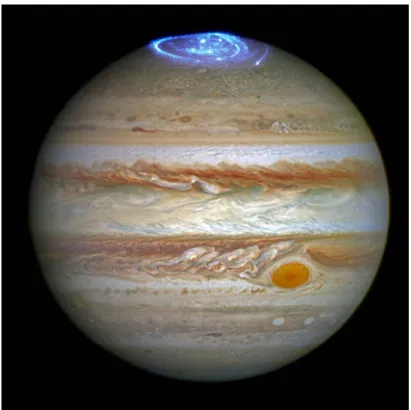
Figure 1.8: Vivid auroras in Jupiter’s atmosphere captured by Hubble Space Telescope, Credits: NASA, ESA, and J. Nichols (University of Leicester)

Jupiter is the largest, most massive planetary object in the solar system, having more than twice the mass of all the other planets combined [29].

Unlike the inner planets of our solar system, there is no indication for the existence of a surface as we know it in Jupiter or in the other gas giants. As we dive deeper in the atmosphere of Jupiter, both temperature and pressure rise which leads to exotic physical state transitions in the interior of the planet. Since most of these transitions appear to be continuous, any kind of surface is not expected in Jupiter [29].

1.3.1 Jupiter’s Atmosphere

Composition

Jupiter is the giant planet that most closely approximates a proto-solar composition, but the abundance of heavy elements such as carbon or nitrogen are three to five times greater than what would be expected in a purely solar composition atmosphere. Pointing to Jupiter initially forming from icy planetesimals, which became massive enough to attract a very large quantity of the surrounding nebula gas [29]. Table 1.4 shows the composition of Jupiter with respective mole fractions and measurement techniques.

Gas Mole fraction Measurement technique

He 0.135 Galileo probe GPMS and HAD

NH3 (5.74 ± 0.22) × 10−4 at deep levels from 8.9-11.7 bar Galileo probe GPMS

H2S (7.69 ± 1.81) × 10−5 Galileo probe GPMS

H2O (4.23 ± 1.38) × 10−4 at deep levels and increasing Galileo probe GPMS

CH4 (2.04 ± 0.49) × 10−3 Galileo probe GPMS CH3D 1.8 × 10−7 Ground-based 5 µm PH3 (1.04 ± 0.10) × 10−6 Cassini mid-IR Ne 1.99 × 10−5 Galileo probe GPMS Ar (1.57 ± 0.35) × 10−5 Galileo probe GPMS Kr (8.04 ± 3.46) × 10−9 Galileo probe GPMS Xe (7.69 ± 2.16) × 10−10 Galileo probe GPMS

AsH3 2.4 × 10−10 (5-8 bar) Ground-based 5 µm

GeH4 4.5 × 10−10 (5-8 bar) Ground-based 5 µm

CO (1.0 ± 0.2) × 10−9 at 6 bar Ground-based 5 µm

HCN >8 × 10−9 at peak at 45◦S Ground-based mid-IR

C2H6 ∼ 4 × 10−6 (5 mbar) increasing by factor of ∼2 towards poles Cassini mid-IR

C2H2 ∼ 4 × 10−8 (5 mbar) at 20◦N, decreasing to ∼1 × 10−8at poles Cassini mid-IR

C4H2 Detected Cassini mid-IR

C2H4 3 × 10−10 (∼10 mbar) Mid-IR and modeled

CH3C2H 2 × 10−10 (∼10 mbar) Mid-IR and modeled

C3H8 2.6 × 10−8 (5 mbar) Ground-based IR

CH3 Detected Cassini mid-IR

CO2 3.5 × 10−10 at p < 10 mbar ISO/SWS

HF < 2.7 × 10−11 Cassini far-IR

HCl < 2.30 × 10−9 Cassini far-IR

HBr < 1.00 × 10−9 Cassini far-IR

HI < 7.60 × 10−9 Cassini far-IR

Table 1.4: Composition of Jupiter. Table excerpt taken from [29]

Structure

Since the lower boundary of the atmosphere is ill-defined, the pressure level of 10 bars, at an altitude of about 90 km below 1 bar with a temperature of around 340 K, is commonly treated as the base of the troposphere [32]. Below the 1 bar level, the troposphere is mainly characterised by several cloud decks dominated by different chemical species. Close to the 5 bar pressure level, there is a good amount of evidence indicating the existence of the water cloud deck and a base in the 6-7 bar layer [29, 33]. Below this level until the 1 bar pressure level the bulk of Jupiter’s interior is expected to be convective and the simplest model tells of a dry adiabatic profile [32, 33].

From 300 mbar, upwards into the atmosphere a statically stable stratosphere seems to be present. Here, haze layers seem to settle and combine with ammonia clouds contaminated with hydrocarbons and possibly the phosphorus allotrope which could give a reddish colour to this layer of clouds in some regions. These contaminators are believed to be generated in the upper stratosphere (1-100 mubar) from the photolysis of methane [29].

At pressures lower than 1 µbar we find the thermosphere. In this region charged particles of the magnetosphere cause dissociation and ionization of the present molecules. Molecular diffusion becomes dominant over convective mixing due to densities being low, leading to large

mean free paths between collisions. Powerful aurorae (see Figure 1.8) are triggered in the polar regions due to this interaction with charged particles [34].

Dynamics

The theories regarding the dynamics of the Jovian atmosphere can be broadly divided into two classes: shallow and deep. The former hold that the observed circulation is largely confined to a thin outer (weather) layer of the planet, which overlays the stable interior. The latter hypothesis postulates that the observed atmospheric flows are only a surface manifestation of deeply rooted circulation in the outer molecular envelope of Jupiter [35].

Shallow models assumed that the jets on Jupiter are driven by small scale turbulence, which is in turn maintained by moist convection in the outer layer of the atmosphere (above the water clouds). The production of the jets in this model are due to the merging of small turbulent structures (vortices) to form larger ones. The finite size of the planet means that the cascade can not produce structures larger than some characteristic scale (Rhines scale). However, these models produce a strong retrograde (subrotating) jet, contrary to observations, despite success-fully explaining the existence of a dozen narrow jets. Also, the jets tend to be unstable and can disappear over time. These also fail to explain how the observed atmospheric flows on Jupiter violate stability criteria [35]. Observations from the Galileo Probe found that the winds on Jupiter extend well below the water clouds at 5–7 bar and do not show any evidence of decay down to 22 bar pressure level. This implies that circulation in the Jovian atmosphere may in fact be deep and not shallow [33].

The deep model was first proposed by Busse in 1976. His model was based on that in any fast-rotating barotropic ideal liquid, the flows are organized in a series of cylinders parallel to the rotational axis. The conditions of the theorem are probably met in the fluid Jovian interior. Therefore, the planet’s molecular hydrogen mantle may be divided into cylinders, each cylinder having a circulation independent of the others. Those latitudes where the cylinders’ outer and inner boundaries intersect with the visible surface of the planet correspond to the jets; the cylinders themselves are observed as zones and belts [35].

The deep model easily explains the strong prograde jet observed at the equator of Jupiter; the jets it produces are stable and do not obey the 2D stability criterion, however, it has major difficulties: It produces a very small number of broad jets; assumes that the molecular hydrogen mantle is thinner than in all other models, occupying only the outer 10% of Jupiter’s radius while in standard models of Jupiter’s interior, the mantle comprises the outer 20–30%; has problems with the driving force of deep circulation, for the deep flows can be caused both by shallow forces or by deep planet-wide convection that transports heat out of the Jovian interior [35].

A banded structure with bright white regions (zones) and darker brown/reddish bands (belts) with prominent zonal jets between zones and belts dominate the visible atmosphere of Jupiter. Both band types flow in different directions with zonal winds that reach 150 m/s, with greater intensity towards the equatorial zones and belts. Individual features like the Great Red Spot (GRS) tend to have the same vorticity as the band in which they are placed [33].

The variable nature of the belts sometimes results in small convective events that grow to great heights and encircle the planet, despite Jupiter’s banded structure being globally stable over centuries of observation. Also, the boundaries between bands and belts may change slightly in latitudinal extent [33].

1.3.2 Exploration of Jupiter

History of Jupiter’s Exploration

Jupiter was first observed through a telescope by Galileo Galilei in 1610 who discovered its four largest moons (Io, Europa, Ganymede and Callisto).

In December 1973, Pioneer 10 flew past Jupiter followed by Pioneer 11 a year later. Provid-ing the first ever close-up images of the visible layers of the atmosphere .

In 1979, both Voyagers flew past the jovian system and improved our understanding of the Galilean moons. They observed volcanic activity for the first time outside the Earth, discovered two satellites (Adrastea and Metis) and the Jupiter ring system.

In 1992, the Ulysses solar probe flew past Jupiter’s north pole performing several measure-ments of the planet’s magnetosphere as it preformed a swing maneuver to attain the desired high inclination orbit to perform around the Sun.

On December 7th 1995, Galileo, the first orbiter mission to Jupiter, arrived in orbit and encircled the planet until 2003. It also witnessed the impact of the Comet Shoemaker-Levy 9 as the spacecraft approached the Jovian system in 1994.

In 2000 the Cassini probe passed by Jupiter on its way to Saturn and provided the highest resolution images of the jovian atmosphere to date (at that time).

In 2007, the New Horizons mission to Pluto flew by Jupiter and studied the less known moons like Amalthea, Himalia and Elara.

In 2011, Juno was launched and entered Jupiter’s orbit in July 2016. This particular orbit takes the spacecraft within 5000 km above the planet’s cloud tops to avoid the hazardous radi-ation environment during the mission and also to study with unprecedented detail the interior structure of Jupiter.

Chapter 2

Methods and Tools

2.1

Radiative Transfer

To analyse the radiation spectrum it is necessary to understand the thermal structure of the atmosphere of the planet of interest. For this, the parallel plane model is used and it is also assumed axial symmetry around the atmosphere’s vertical axis as a first approach. The model assumes that the atmosphere may be represented by a sucession of parallel, plane, and homogeneous layers superimposed on one another locally. Under these conditions, the radiative transfer equation is given by [6]:

µdIν dτν

= Iν− Jν (2.1)

where µ = cos θ, θ being the angle between the line of incidence and the vertical, Iν is the specific

intensity (a function of frequency ν), τ_ν is the optical thickness above the level of altitude z, and J_ν is the source function. With the coefficient of absorption K_ν and the density ρ, we have [6]:

τν=

Z ∞

z

Kνρdz (2.2)

We have local thermodynamic equilibrium for pressures above 1 mbar. In these conditions the populations at different energy levels obey Boltzmann’ s law, the physical properties of the medium depend only on the temperature and the velocity distributions of the atoms and molecules are Maxwellian. So our source function becomes the Planck function [6].

Afterwards, we need to solve an energy conservation equation reduced for radiative equilib-rium in order to determine the thermal structure of the atmosphere. This equation gives us the temperature of a level z [6]: X ν X z0 X µ B(T0)e−τ0/µ= σT4 (2.3) where T’ is the temperature at at layer z’ and τ0 is the optical thickness between z and z’ [6]:

τ_ν0 = Z z0

z

Kνρdz (2.4)

This radiative equilibrium equation is constrained by the law of hydrostatic equilibrium and the perfect gas law. Which gives us the following equation for pressure when combined for an isothermal atmosphere [6]:

where H = RT /µG is the scale height, µ the mean molecular mass, R is the universal gas constant, G is the gravitational constant and z0 is a reference level [6].

For a planet with a surface and a tenuous atmosphere, the reflected solar light is diffused by the surface following Lambert’s law [6]:

F (θ) = F cos(θ0) (2.6)

where F is the flux arriving at the surface, θ0 is incidence angle, measured relative to the normal

to the surface, and θ the angle of the normal with the direction of diffusion [6]. If one knows the angle that the incident radiation makes with the normal to the surface, it is then possible to deduce the number of molecules along the line of sight [6]. This radiation, in visible and in the near infrared, will have lines that will correspond to vibration-rotation transitions of these said molecules [6]. By comparing the intensities in several absorption lines belonging to the same component, one can have an estimate of the average temperature of the medium. If the lines are widened due to the pressure of the medium, one also can estimate the pressure of said medium by measuring the width of the line, as long as the instrument’s spectral resolution is high enough [6]. Otherwise, one can only deduce the average temperature by the general shap of the absorption band [6].

If the planet has a dense atmosphere, we start to have scattering phenomena [6]. So, one requires knowledge of density, the distribution as a function of altitude, the absorption and extinction coefficients, and the scattering phase function for each type of scattering particle [6]. If the information about all these data is not available, one uses the reflecting layer model (RLM), where a dense, cloud layer is considered equivalent to a surface covered by a clear atmosphere, with no scattering [6].

The thermal component is more complicated to analyse from the ground, due to it laying in the infrared [6]. However, due to being less affected by scattering effects it is easier to study from a theoretical point of view [6]. Assuming local thermodynamic equilibrium, the emergent flux is given by the transfer equation[6]:

Φν= Z µ Z ∞ z0 B(z, ν)eτν(z)/µ_{dτ (µ)/µ (2.7)}

For the case of a tenuous atmosphere, the altitude z0 may refer to the altitude of the surface, or

to a sufficiently deep layer for the exponential to be negligible in the case of dense atmospheres [6].

The brightness temperature TB(ν) is a good parameter to measure the emergent flux Φν,

because there is a simple relationship between the brightness temperature and the optical thick-ness, the Barbier-Eddington approximation [6]:

• The brightness temperature is the temperature of the atmospheric layer for which the optical thickness is equal to 1 in the case of the specific intensity emitted along the vertical;

• The brightness temperature is the temperature of the atmospheric layer for which the optical thickness is equal to 0.66 in the case of the flux emitted over the whole of the disk;

function is maximum, defined by its optical thickness [6]:

F P (ν, z) = e−τν(z)/µ1 µ

dτν(z)

dz (2.8)

which leads to the flux being expressed as a function of FP(ν,z): Φν = Z µ Z ∞ z0 B(z, ν)F P (ν, z)dz (2.9)

2.2

UVES - Ultraviolet and Visual Echelle Spectrograph

UVES is a cross-dispersed echelle spectrograph designed to operate with high efficiency from 300 nm to about 1100 nm. It is installed on Nasmyth B focus of the Unit Telescope 2 (UT2) of the the Very Large Telescope (VLT). Inside the spectrograph the light beam from the telescope is split in two arms (UV to Blue,and Visual to Red). These two arms can be operated in parallel via a dichroic beam splitter or separately. When a 1-arcsec slit is used, it possesses a resolving power of about 40,000 and the maximum (two-pixel) resolution is 110,000 or 80,000 in the Red-and the Blue Arm, respectively. Three image slicers are also available to obtain high resolving power without excessive slit loss. The instrument allows for accurate wavelength calibration due to being built for maximum mechanical stability. It also allows for an iodine cell to be inserted in the light beam for observations requiring extremely high accuracy [36, 37].

The red arm covers light from 420 nm to 1100 nm and is equipped with a CCD mosaic made of an EEV chip and a MIT chip while the blue arm of UVES covers light from 300 nm to 500 and is equipped with an EEV CCD [37].

2.3

ISO – The Infrared Space Observatory

ISO was the world’s first true orbiting infrared observatory. It was equipped with four scientific instruments: ISOCAM, ISO’s infrared camera, that covered the wavelengths between 2.5 and 17 microns with two different detectors, the short wavelength (SW) detector (2.5–5.5

µm) and the long wavelength (LW) detector (4–17 µm); ISOPHOT, ISO’s photo-polarimeter,

which handled the 2.5 to 240 microns wavelength range; SWS, the Short-Wave Spectrometer, that covered the 2.4 to 45 micron band; LWS, the Long-Wave Spectrometer, which handle the 45 to 196.8 micron wavelenght range [39].

2.4

The IA’s High-Resolution Spectroscopy Pipeline

The pipeline operates on .fits image files. These files are arrays with a value proportional to the amount of photons that hit that pixel associated to each pixel position. These images also possess a header, which is image metadata that has relevant information about the images.

The first step of the pipeline is to create a database of all the images files, this includes science and calibration files. Next, it checks if said image files are present in the working directory. This is the directory where all the subsequent files and folders will be created. Afterwards, it checks if there is a median bias and median flat file, if these files are not present, the pipeline creates them by taking all the images (flats for median flat and bias for median bias) and calculating the median of the values in the same position in the arrays for all the array positions.

On the completion of this procedure, the pipeline commences importing the image files and at the same time subtracting them by the median bias, in other words, performing a bias calibration, correcting the pixel-to-pixel zero point variation. After completing this step, the pipeline maps the location of each spectral order of the instrument in the images. Then it proceeds to remove scattered light if there is any present and lastly divide the science images by the median flat one in order to do a flat field calibration, removing image artefacts due to optical effects.

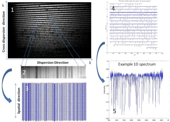
Finally, the pipeline builds the 1D spectrum. This is done by taking all the spectral orders and all the pixels that have light (given by the order definition file) and associating them a wavelength value. These values are generated based on very well known lines of a ThAr lamp that is present in UVES. Knowing the pixel position of these lines on the images, the pipeline extrapolates the wavelength values to the rest of the pixels. Lastly, the pipeline places the different spectral orders side by side to have a continuous plot.

Figure 2.3 shows the various stages to reach the final plot. Starting with the echelogram (1), proceeding into taking the data into the scripts environment (3), account for the cross dispersion and plotting intensity as a function of pixel (4), putting them side by side and attributing a wavelength value for each pixel (the values of the intensity have a constant added to them so that all the orders aren’t plotted on top of each other). (The plot 5 is just one of the spectral orders of plot 4)

The pipeline goes on to take into account the shape of the target and the dispersion relations in order to calculate the Doppler shifts in each point of the target image and calculate the wind velocity, but that isn’t the focus of this work

2.5

EsoReflex: UVES pipeline

EsoReflex (ESO Recipe Flexible Execution Workbench) is an environment built using the Kepler workflow engine, which itself makes use of the Ptolemy II framework that allows for an easy and flexible way to execute VLT pipelines [40].

Figure 2.4: Esoreflex enviroment

Similar to the IA’s pipeline (section 2.4), EsoReflex UVES pipeline performs the data re-duction of the science files using the calibration data by performing the bias, flat and dark (correction of CCD noise due to temperature effects) calibrations as well as the wavelength calibrations.

To start the pipeline, one must first select the data directories where the data files are (science and calibration), the location of where the temporary files will be saved and where the final files will be created at the end of the pipeline. Afterwards, one needs to choose the type of data extraction in the ”Spectrum Extraction” actor in the ”INIT EXTRACT METHOD” option. The default option is used for point sources, but for extended sources this must be changed to 2d (Figure 2.5).

Figure 2.5: Editing the parameters of the Spectrum Extraction actor for the case of Titan

Next, one initialises the pipeline, a new window will appear asking the user to select the data that one wishes to reduce (Figure 2.6). In this window, the user can inspect each science file to see what calibration files will be used in the pipeline and enable/disable their use in the processing.

Figure 2.6: Window that appears to choose the data to be processed (in this case the Titan data has already been reduced)

After this step, the pipeline runs and new folders will be created in the output directory with the name of the original science files. In each of these folders the output files of the pipeline will be created. These include the 2d spectra (these type of files are the ones used in the detection of chemical species in this work), the 1d spectra and their respective error files.

2.6

HITRAN & ExoMol

HITRAN stands for high-resolution transmission molecular absorption database. It is a compilation of spectroscopic parameters used to predict and simulate the transmission and emission of light in the atmosphere. The database is a long-running project started by the Air Force Cambridge Research Laboratories (AFCRL) in the late 1960s in response to the need for detailed knowledge of the infrared properties of the atmosphere [41].

To use the database, one simply needs to create an account to have access. To search for the relevant chemical species, the user selects line-by-line search and then ticks the chemical species of interest. Afterwards the user proceeds to select the isotoplogues and the wavenumber range in cm−1 that he/she is interested in. Finally the user selects or creates an output format and in return get text files with the information the user is interested in aswell as the references. In the case of this work, the information of interest will be the wavenumber and the line intensity. Similarly to HITRAN, ExoMol is a database of molecular lines lists that can be use for spectral characterisation and simulation. However, its tailored to high hot exoplanets, brown dwarfs and cool stars [42], but there are some transition lines list for some molecules at room temperature.

To use this database one can search by data type sets or by molecule. Next, one chooses the molecule of interest and the isotopologue. And finally, the user chooses what data set he/she wants. Unlike HITRAN, you cant choose multiple molecules, isotopologues or the wavelength range of your interest, you must search the available files with established wavelength ranges in the database. Thus, making the search for the relevant information more tedious and time consuming.

2.7

Flux Calibration

The spectra don’t have physical values for flux when they are obtained. These values are proportional to the number of photons that hit the CCD during the measurements. However, that proportion is unknown. In order to obtain physical quantities one must perform a flux calibration, starting by obtaining the specific response function of the instrument. To do this, a calibration star near our target must be observed during the observations, in order to ensure the atmospheric conditions are roughly the same. The response function will be the quotient between the expected star spectrum and the one measured with our instrument:

Response f unction = Expected Star f lux

M easured Star f lux (2.10)

Using Figure 2.7 as an example, we see the difference between the expected flux of Piscium and what was measured with the HARPS instrument.

Figure 2.7: Absolute flux of reference star Piscium as a function of wavelength in micrometres. (Left plot). Measured flux of the same star by the HARPS north instrument.

Dividing the expected spectrum by the measured spectrum as show in the equation 2.10 we get the response function of HARPS, as show in Figure 2.8

Figure 2.8: Response function of the instrument HARPS north

Lastly, we multiply the response function by the spectra of our target, obtaining flux cal-ibrated spectra with physical units of flux. Figure 2.9 shows the initial wavelength calcal-ibrated spectrum of Venus measured with HARPS and the same spectrum after being flux calibrated.

Figure 2.9: Venus spectrum obtained by the HARPS north instrument with arbitrary units of intensity as function of wavelength (Left plot). Venus spectrum calibrated using the response function with absolute units of intensity as function of wavelength (Right plot)

Chapter 3

Observations

3.1

Titan

Titan was observed using blue arm of UVES of the VLT over the course of 4 hours on the 21st of June 2018. These observations, that were a collaboration with the University of Bordeux, were made with the purpose to detect the presence of the C₃ molecule on Titan’s atmosphere by detecting absorption lines on the spectra. However, in this work we go beyond that objective. Using HITRAN, we searched for all known molecules that make up Titan’s atmosphere that are available on the HITRAN database on the wavelength range of UVES’s blue arm. In these conditions only H2 , HD and H2O16 data was retrieved from HITRAN.

The data reduction of the science image files of Titan was done using the EsoReflex UVES pipeline. Afterwards we proceeded to create a mean spectra of Titan, by adding them all together and dividing each value of intensity by the amount of spectra (22). This is done in order to improve the signal-to-noise ratio of the spectra. Thirdly, we checked this mean spectra and saw what pixels had Titan on them and the pixels that were just sky. The central pixel was the 19th and Titan was covered by about 4 pixels in each direction, from the 15th to the 23rd pixel. Again, we performed another mean of the spectra, by taking all the values of intensity that correspond to these pixels, adding them and dividing the values by the amount of pixels (9). This final mean spectra is the spectra that the chemical species detections were performed on.

3.2

Saturn

The Saturn data came from two sources, the first came from UVES red arm observations, the second from the SWS on board ISO spacecraft.

The UVES Saturn data was provided to me by my supervisor already wavelength calibrated using the IA’s High-Resolution Spectroscopy pipeline. These 29 spectra were measured on the 20th of April 2004. They, like the ones of Titan, were used to create a mean spectra. We took this mean spectra and added all spectra from all the pixels that covered Saturn and divided the value of the intensity by the amount of pixels (31), in order to improve the signal-to-noise ratio. This final spectra is the one that was used for the detection of CH₄.

The ISO Saturn data was provided by Doctor Th´er`ese Encrenaz (Paris Observatory). This data covers 12.5 to 16.2 micrometre wavelength range, and is already flux and wavelength calibrated. This data was used to detect the C₄H₂ molecule.

3.3

Jupiter

The Jupiter data was also provided by Doctor Th´er`ese Encrenaz (Paris Observatory) and was also observed with the SWS of ISO spacecraft. This data consists of two spectra, one that covers the 2.3 to 3.2 micrometre wavelength range and another that covers the 3.2 to 12.6 micrometre wavelength range. This data was used for the detection of CH₄, NH₃ and H+₃

Chapter 4

Results

4.1

Titan

4.1.1 H2O

Using HITRAN to search for the transition lines for each molecule, this is the output from the database between 20000 and 33333 cm−1 (300 and 500 nm) wavenumber range for H₂O:

Figure 4.1: Output of HITRAN for H2O transition lines

With this information and taking into account the mean Doppler redshift of 0.3 ˚A due to the relative motion of Titan with respect to the Earth calculated using the velocity from Horizons Web Interface [43], the following possible absorption lines for water were detected:

Figure 4.2: Telluric H2O absorption line at 3993.17 ˚A and Titan’s at 3993.37 ˚A