Semi-Automated Workflow for Natural
Disaster Assessment: A Case Study of
Banda Aceh, Indonesia
Semi-Automated Workflow for Natural
Disaster Assessment:
A Case Study of Banda Aceh, Indonesia
Dissertation supervised by:
PhD Mario Caetano,
PhD Marco Painho,
PhD Ignacio Guerrero,
ACKNOWLEDGNEMENTS
I would like to thank my supervisors Mario Caetano, Marco Painho and
Ignacio Guerrero for their continued feedback, support and guidance during
the course of the dissertation.
I would also like to thank my family for their continued support and
Semi-Automated Workflow for Natural
Disaster Assessment:
A Case Study of Banda Aceh, Indonesia
ABSTRACT
The past decade has witnessed many natural disasters hitting highly populated areas
causing billions of dollars in damage as well as many human casualties. During natural
disasters, when attaining ground measurements are limited, remote sensing and
geographical information systems (GIS) are useful tools for in-depth analysis of the
affected area. This report will introduce a new semi-automatic workflow in which the
road network will be used to break up the area into “blocks” and then zonal statistics
will be applied to detect change based on the created blocks rather than the conventional
methods of change detection; pixel by pixel and object oriented. This hybrid approach
will take advantage of the simplicity and ease of applying pixel change detection
methods on fixed objects or “blocks” to assess for damage. The change detection
analysis results can then be used to map and quantify damage caused by natural
disasters using pre and post Landsat imagery of the affected area. Multi-Criteria
Analysis is performed on the damage map, proximity to roads, proximity to waterbodies
and building size to find the most suitable locations for temporary housing sites.
The image differencing of NDWI mean produced the highest overall accuracy of
71.70% among eleven bands/indices and the multi-criteria analysis successfully
selected fourteen temporary housing center sites from a possible 114. When time is of
essence with limited resources and GIS expertise on the field, local authorities can
KEYWORDS
Disaster Management
Damage Assessment
Natural Disaster Change Detection
Multi-Criteria Analysis
ArcGIS
FME
ACRONYMS
LULC
–
Landuse Landcover
IDNDR
–
International Decade for Natural Disaster Reduction
GIS
–
Geographic Information Systems
TM
–
Thematic Mapper
NDVI
–
Normalized Difference Vegetation Index
NDBI
–
Normalized Difference Build-up Index
NDWI
–
Normalized Difference Water Index
MCA
–
Multi-Criteria Analysis
OSM
–
Open Street Map
DMSG
–
Disaster Management Support Group
WHO
–
World Health Organization
UN
–
United Nations
NIMS
–
National Incident Management System
MLC
–
Maximum Likelihood Classifier
PCA
–
Principle Component Analysis
SVM
–
Support Vector Machine
NN
–
Nearest Neighbor
MCDA
–
Multi-Criteria Decision Analysis
NIR
–
Near Infrared
ETM
–
Thematic Mapper Plus
MNDWI
–
Modified Normalized Difference Water Index
SAVI
–
Soil Adjusted Vegetation Index
INDEX OF TEXT
ACKNOWLEDGNEMENTS
... iii
ABSTRACT
... iv
KEYWORDS
... v
ACRONYMS
... vi
INDEX OF FIGURES
... ix
INDEX OF TABLES
... xi
1
INTRODUCTION
... 1
1.1 Overview ... 1
1.2 Objectives ... 3
2
THEORETICAL FRAMEWORK
... 4
2.1 Remote Sensing for Disaster Management ... 4
2.1.1 Four Phases of Emergency Management ... 6
2.1.2 Rapid Mapping ... 8
2.1.3 Automated Workflows for Mapping ... 11
2.1.4 Specialized Indices ... 12
2.2 Change Detection Overview ... 14
2.3 Multi-Criteria Decision Analysis (MCDA) ... 16
3
STUDY AREA And DATA
... 19
3.1 Data ... 20
3.1.1 Reference Disaster Map ... 21
3.1.2 Reference Temporary Living Centers (TLC)... 23
4
METHODOLOGY
... 24
4.1 Pre-Processing ... 26
4.1.1 Image ... 26
4.1.2 Open Street Map Data ... 27
4.2 City Block Creation from Roads ... 27
4.3 Zonal Statistics and Change Detection ... 31
4.4 Map Creation ... 36
4.5 Multi-Criteria Decision Analysis ... 37
4.6 Accuracy Assessment ... 41
4.6.1 City Boundary ... 41
4.6.2 Disaster Maps ... 42
5
RESULTS AND DISCUSSION
... 46
5.1 City Blocks ... 46
5.2 Accuracy Assessment ... 47
5.2.1 City Boundary ... 47
5.2.2 Disaster Maps ... 48
5.2.3 Pixel Based Map ... 53
5.3 Final Map ... 55
5.4 Most Suitable Temporary Living Sites ... 56
5.5 Online Map ... 57
6
CONCLUSION
... 58
7
BIBLIOGRAPHY
... 61
8
APPENDICES ... 66
8.1 APPENDIX 1 – Confusion Matrices ... 67
8.1.1 Image Differencing ... 67
INDEX OF FIGURES
Figure 1- Number of People Affected by Natural Disaster (UNDP 2004) ... 5
Figure 2
–
Four Components of Emergency Management (Safety 2010) ... 7
Figure 3
–
Number of Days Taken To Produce First Crisis Map (Allenbach 2005) ... 9
Figure 4
–
Flowchart of Crisis Mapping (Allenbach 2005) ... 10
Figure 5
–
Change Detection Approaches ... 14
Figure 6
–
Simple Change Detection Calculations (Differencing vs Ratioing) ... 15
Figure 7
–
Example of Multi-Criteria Evaluation Structure (Eastman 1995) ... 17
Figure 8
–
Epicentre of 2004 Indian Ocean Tsunami and Countries Affected
(Worldatlas) ... 19
Figure 9
–
Map of Banda Aceh, Indonesia ... 20
Figure 10
–
Banda Aceh Damage Map by SERTIT ... 22
Figure 11 - UN Temporary Living Centres (Reference Map) ... 23
Figure 12
–
Overview of Semi-Automated Workflow for Damage Assessment ... 25
Figure 13
–
Clipped Landsat Imagery to Banda Aceh, Indonesia ... 26
Figure 14
–
The Script Workflow of Creating City Blocks and Tool Interface ... 28
Figure 15
–
First Iteration of City Blocks and Block Areas ... 28
Figure 16
–
The Block Size Iteration Workflow ... 29
Figure 17
–
City Blocks and Block Size after Iteration Process ... 29
Figure 18
–
FME Script for Road Density and Tool Interface ... 30
Figure 19
–
The Creation of the City Boundary ... 31
Figure 20
–
FME Script to Compute Change Detection ... 33
Figure 21
–
FME Script for Change Detection Calculation
–
Part 1 ... 34
Figure 22 - FME Script for Change Detection Calculation
–
Part 2 ... 35
Figure 23 - FME Script for Change Detection Calculation
–
Part 3 ... 35
Figure 24
–
Varying Damage Patterns from Six Bands of Landsat (Image
Differencing) ... 36
Figure 25
–
Normalized Suitability Scores for Each Factor ... 38
Figure 26
–
Multi-Criteria Analysis Script Workflow ... 39
Figure 27
–
Suitability Map for Temporary Living Centre created by MCA ... 40
Figure 28- Finding Ideal Locations for Temporary Living Centres Tool Interface .... 40
Figure 29
–
City Boundary Obtained from Roads Compared with Administrative
Boundary ... 41
Figure 31
–
FME Script to Transfer Reference Damage Data to Blocks and Tool
Interface ... 43
Figure 32- City Blocks with Reference Damage Data ... 44
Figure 33- Final City Blocks ... 46
Figure 34
–
Final Block Size Compared Against Average ... 47
Figure 35- Final City Boundary Derived from Roads ... 47
Figure 36- Image Differencing Overall Accuracies ... 49
Figure 37
–
Image Ratioing Accuracies ... 50
Figure 38- Ratio Accuracies vs Differencing Accuracies ... 51
Figure 39-
NDWI Mean, User’s, Producer’s
Accuracies for All Damage Levels ... 52
Figure 40- Overall accuracy vs Extreme and Low Damage for All Bands/Indices ... 53
Figure 41- Damage Map Derived from Pixel by Pixel Differencing ... 53
Figure 42- Pixel Classification Result ... 54
Figure 43- Final Damage Map ... 55
Figure 44- Temporary Housing Sites Map ... 56
Figure 45
–
Online Damage Map (top left), Differencing Change Detection Values
(top right) and Close-up of Selected Temporary Housing Site (bottom) ... 57
INDEX OF TABLES
1
INTRODUCTION
1.1
Overview
The increase in readily available remote sensed data from satellites and aerial photography has developed into an essential tool for resource and disaster management as well as many other applications (Weih Jr 2010). Remote sensed data has increased the speed, precision and cost efficiency of forming spatial analysis for a particular purpose as well as development of spatial
pattern maps that previously wasn’t possible without ground truth samples (McRoberts 2007). With the increasing availability of satellite data, many large-scale specialized methods have been developed using change detection for forest cover change (Fraser R.H. 2005) and burned areas estimation (Gitas I.Z. 2004). Another area where remote sensing is prominently used is in mapping changes due to urbanization and urban sprawl (Xian 2005).
The traditional multispectral classification methods used for urban change produces reasonable results, mainly below 80%, because of the nature of the urban class being heterogeneous and causing spectral confusion. In order to improve the classification accuracy, many methods have been formed that incorporate different procedures to improve built-up area abstraction (Dehvari 2009). The built-up areas of Washington D.C. was extracted with 85% accuracy using unsupervised classification method on NDVI differencing of multi-date Landsat imagery (Masek 2000). Another approach that combined multiple techniques was applied by Xu (2002), who used a supervised classification with mixture of signature analysis to select built-up areas in Fuqing City, China. The author improved the overall accuracy by incorporating the classification layer with the difference in spectral response between urban and non-urban classes. Xian (2005) produced accuracy of over 85% by combining an unsupervised classification with regression tree algorithm classification of build-up areas to measure the extension of built-up areas into watersheds in Florida.
a “salt and pepper” effect that adds to the imprecision regarding the overall classification
accuracy (Campagnolo 2007).
The possibility of creating a fully automated classification methods that would be an improvement over the pixel-based techniques that has been looked at for years (Blaschke 2000). Various computer software packages are created to analyze the characteristics of a pixel in a more object oriented manner which takes both the spectral and spatial properties. Feature Analyst and eCognition are two of the most widely used software packages that perform object-based classification in which a segmentation procedure coupled with iterative learning algorithms are applied to form a semi-automated classification process that has proven to be more accurate when comparing with pixel-based techniques especially with the availability of high resolution imagery (Blundell 2006).
It’s important to note, in spite of advancements in satellite imagery provisions raw satellite
imagery is essentially unusable for non-expert users such as emergency relief workers or decision makers. For the created products to be fully understood by non-experts, damage maps, reports and statistics have to be obtained from processing, analysis and interpretation of the raw data by a GIS expert. One of the most important, frequently overlooked aspect of data processing and delivery is the direct interaction with the emergency assessment team and decision makers. Without a proper and concise explanation of the sophisticated image analysis, mapping and GIS products there is little meaningfulness derived from the products for the
emergency response team. It’s as important to produce easily understandable products or to
provide close contact concerning image analysis in order for non-GIS users such as decision makers to maximize the intake of the intended information of the products to make the appropriate decisions (Voigt 2007).
This report will introduce a new semi-automatic workflow in which the road network will be
used to break up the area into “blocks” and then zonal statistics will be applied to detect change based on the created blocks rather than a pixel by pixel or object oriented method. This hybrid approach will take advantage of the simplicity and ease of applying pixel change detection
methods on fixed objects or “blocks” to assess for damage. The change detection analysis
results can then be used to map and quantify damage caused by natural disasters using pre and post Landsat imagery of the affected area. With the addition of auxiliary OSM data, more specific spatial analysis can be done for emergency response purposes such as locations of temporary housing sites during a disaster. When time is of essence with limited resources and GIS expertise on the field, local authorities can greatly benefit from a rapid generalized analysis
that will provide a “bird-eye view” of the affected area to efficiently and effectively allocate emergency efforts within a short time frame.
1.2
Objectives
The objective of this research is to develop a semi-automated workflow to assess and quantify natural disaster damage. The accuracy results of two of the most commonly used pixel-change detection (ratio and differencing) methods will be compared based on artificially derived city
evaluate which one produces the most accurate map. To further add supplementary value to the disaster damage map for emergency response purposes, using multi-criteria analysis (MCA) with the addition of auxiliary data (Open Street Map (OSM) data), the most suitable temporary housing sites will be selected to accommodate displaced individuals during a disaster.
2
THEORETICAL FRAMEWORK
2.1
Remote Sensing for Disaster Management
The advancement of remote sensing satellite systems and image-analysis methods in recent times have made earth-observation systems an integral part of emergency management for natural and humanitarian crisis situations (G. Bitelli 2001). The rapid improvements in coverage, spatial and temporal resolution of satellite imagery have attributed to this, as such:
a) Spatial resolution or pixel spacing has improved to a few meters precision for optical and radar data.
b) International satellite-based disaster-response possibilities have enhanced due to the rapid increase in communication, interoperability and networking between different satellite organizations as well as the increase in data derived from satellites.
c) Increase in number of international disaster research agencies such as Disaster Management Support Group (DMSG) and International Charter Space and Major Disasters (Eguchi 2001).
The plain observation and monitoring of present and future natural disasters was one of the main tasks of this international initiative, with the overall intention of enhancing the emergency management process. The various international disaster monitoring agencies combined are referred to as International Charter (Charter 2000). On a yearly basis, natural disasters are responsible for billions of dollars in property and economic damage as well as casualties numbering in the thousands. A study by the World Health Organization (WHO) showed that the nineteen years between 1964 and 1983 approximately 2.5 million people died from natural disaster events as well as displacing an additional 750 million. Due to the increasing concentration of people living in urban and coastal areas highly susceptible to the dangers of natural disaster events, initiatives had to be taken to reduce the impact of natural hazards (Voigt 2007). With the rapid advancement of both scientific and technological research and the availability of almost instantaneous satellite data, this provided unique opportunities to mitigate the impacts of natural disasters. The United Nations (UN) passed a resolution (1987) declaring
of the resolution was for ‘the international community to pay special attention to fostering cooperation in the field of natural disaster reduction’. The UN resolution put forward the development of internationally cooperated strategies to decrease loss caused from natural disasters by focusing on different aspects of disaster management such as prevention and preparedness plus improving efforts designated to disaster relief, response and recovery (NDR 1991).
As of the year 2000, it was estimated that at least 75% of the world’s population lived in areas at risk from a major disaster (UNDP 2004). And because these high-risk areas periodically experience major disasters, it is a logical connection to say that the number of people who are annually affected by disasters is equally high ((ISDR) 2004)(Figure 1). The number of people moving from rural areas to cities also known as urbanization has increased dramatically over the years. In 1950, around 2.5 billion people lived in cities which accounts for less than 30% of the population compared to 5.7 billion people in 1998 that live in cities, which increased to 45% of the total population. The trend is set to continue according to UN estimates of 2025 which indicates 8.3 billion people will be living in cities, accumulating to 60% of the total population (Economic 2001). The current trend of natural disaster shows that the number of disaster occurrence is rising every year even though there are less human causalities from disaster events, more people are being affected. The reconstruction cost of disaster have become more expensive, with poorer countries experiencing far more economic consequences in the long term than wealthier nations largely due to the fact that rich countries have extra funds to absorb the cost whereas poorer countries reallocate money that was in place for development to absorb the cost, therefore hindering development.
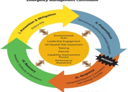
2.1.1
Four Phases of Emergency Management
The occurrence of a natural disasters such as floods, hurricanes, volcanoes, earthquakes, wildfires and other natural hazardous incidents are inevitable. Even though these events have great impacts and can cause catastrophic change within the natural environment, the occurrences are inherently part of the natural system. Natural environments have shown to have incredible resilience when it comes to damage from these events and have shown to regenerate and even restore habitat and ecosystems within a relatively short time period. When man-made
environments are hit by these events, that’s when the term “disaster” is used. The term “disaster” is used when man-made environments influencing human activity such as infrastructure, agricultural fields and other land uses crosses paths with natural forces. The human built environment is not as resilient as the natural one and an entire man-made community can be depleted and require many years to re-establish (Cutter 2003).
• Mitigation actions are designed to reduce the physical and social damages caused from
disaster events and therefore intersects all the phases of emergency management. The objective of this phase is to reduce human casualties and property damage by creating safer communities. This is achieved by risk analysis of the community to enforce specific building codes (constructing disaster-resistant structures), zoning requirements (subdivision regulations to discourage development in high-risk areas) and building artificial barriers such as levees. Education programs aimed to train the public regarding vital emergency procedures and how to protect their property against the forces of nature (USAID/OAS 1997).
• Preparedness actions increase the capability of a community in dealing with a disaster event.
Preparedness is defined as, ‘a continuous cycle of planning, organizing, training, equipping, exercising, evaluating, and taking corrective action in an effort to ensure effective coordination
during incident response,’ by The National Incident Management System (NIMS). Preparedness actions can be broadly divided into two groups, one being structural actions that deal with preparing for the immediate arrival of disaster, for example sandbagging coastal areas and the other being non-structural actions which helps reduce human casualties and property damage. Preparedness stage also deals with the design of the warning systems, improvement of response measures as well as preparing emergency methods and training emergency staff (Lindsay 2012).
• Response actions deals with efficient coordination of resources during or directly after a disaster where time is of essence. The response phase is intended to provide immediate help to the victims in practices such as medical care, food distribution, search and rescue operations and temporary shelter housing. This phase also includes a quick assessment of the affected area in terms of property damage, security and most importantly the victims in danger (Safety 2010).
• Recovery actions help the affected community get back to normal conditions and begins after the disaster has occurred. The emergency management activities include repair of basic services such as restoration of roads, power, water and other essential social, physical and economic damages that are vital for a community to function. In essence, recovery activities are aimed to reduce the effects of insecurity, lack of shelter, disaster, starvation and increasing number of victims (County n.d.).
2.1.2
Rapid Mapping
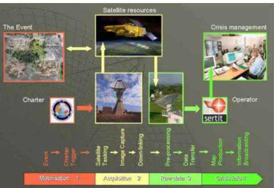
The International Charter on Space and Major Disaster was created in 1999 to encourage international cooperation in terms of civil protection, emergency aid and security during a disaster by utilizing data from governmental satellites and national space agencies. From 1999 to 2006, the International Charter has been triggered over 100 times (Charter 2000) providing valuable information within a short time frame in terms of mapping and analysis products for emergency management. Seven major national space agencies are part of this initiative that make available the data acquired from their satellites once a disaster has occurred, these agencies are: NOAA (USA), ISRO (India), CONAE (Argentina), JAXA (Japan), CNES (France), ESA (Europe) and CSA (Canada). The agency shares a variety of data mostly in optical and radar platforms which include IRS, SAC-C, SPOT, MERIS, ERS, ENVISAT and RADARSAT (CEOS 2002).
The dissemination of fast up-to-date accurate image analysis products during the response and recovery phase of the emergency management cycle is the main focus of the International Charter. In addition, its purpose is to assist with disaster assessment especially in remote areas where attaining ground or other means of data is insufficient. Due to recent efforts of the International Charter, the access, delivery and access of satellite data can be implemented within a short time period (from hours to several days) which allows appropriate, timely and beneficial emergency response in the impact area. The International Charter offers a global mechanism to incorporate data from multiple satellites/agencies within a short timeframe and
During a disaster, the emergency management officials require information regarding the material and human impact as well as the location and the extent of the area affected to enable emergency response. In order to create precise reliable geographical content such as rapid mapping products the utilization and acquisition of Earth Observation (EO) information has to be done swiftly. One agency that provides rapid mapping services is SERTIT (Louis Pasteur University, Strasbourg, France) which works together with the French Space Agency (CNES) and European Space Agency (ESA) to furnish feedback on mapping products. The aim of SERTIT products are to provide valuable geographic information from satellite imagery. EO satellites provide both low and high resolution data that are utilized based on the mapping objective (CEOS 2002). In order for the raw data from multiple sources to be utilized, the data has to be formatted and go through a multi-process that requires the digital data obtained from the satellites to be manipulated and interpreted by remote sensing specialists while also being validated through computer assisted means. The transformation from raw data to geographic data has to done in a short time, since in rapid mapping production time is essential; the production cycle spans hours to days rather than a typical mapping cycle that requires weeks to months. The rapid mapping mission is to produce geographic mapping of areas affected by natural disasters within 12 hours of raw data acquisition by diffusion of all available sensors. Although the focus of the SERTIT is to decrease the time it takes to produce crisis maps, Figure 3 shows that in most cases it takes over 3 days from the time the event happens to the first crisis map. The figure is based on four years span of the Charters actions and with an average of 5 days with some events taking over 10 days, indicating there is much room for improvement in providing rapid crisis maps. The rapid mapping product consists of geo-referenced digital map
that incorporates newly created on-the-fly event map with reference satellite data. Due to its success in providing rapid mapping solutions for floods, this method was further adopted to provide rapid mapping for natural disasters as part of The International Charter on Space and
Major Disaster’s on-call operation service (Allenbach 2005).
Once the Charter is triggered, it goes through four steps until a meaningful map is produced (Figure 4). The first step is mobilisation, its right after the disaster event when the charter is triggered followed by the acquisition step in which the image for the affected area is retrieved, then the pre-processing of the raw data and finally the informative map production. The International Charters products have been very beneficial to the disaster management domain but with increasing rate of disasters, (Voigt 2007) highlighted three areas in which further improvement is required. Firstly, the main product of this initiative is providing raw satellite imagery of the affected area rather than spatial analysis maps (ex. Damage assessment) which should be improved to foster quicker decision making in regards to natural disasters. Secondly, in order to improve migration efforts, the speed of information transfer has to be improved to maximize effective responsiveness. Thirdly, the cooperation, coordination and sharing mechanism between the existing partners need to improve with the aim to more efficiently deal with organizational, technical and data sharing (Charter 2000, Allenbach 2005).
There is a major challenge in the combination of local and global GPS data as well as combination between new and older datasets due to the absence of format standards
(GeoHazards 2004). Some examples of change detection analysis done from multiple sources are:
- Remote Sensing data can be utilized for assessing areas prone to earthquake activity as it provides up to date spatially continuous data on the tectonic landscape which can be used to better understand local fault systems. Using the capabilities of remote sensed data fused with ground data can provide better approximation of displacements and regional slip models of tectonic tension levels (Z. Cakir 2003).
- Combination of demographic data with a building infrastructure dataset and imagery to assess vulnerability and create post-disaster damage assessment for an area stricken by an earthquake (Rejaie 2004).
- To greatly reduce spectral confusion between urban and non-urban classes, Zhang (2002) performed post-classification change detection of Beijing, China by combining road density with information obtained from spectral bands which improved overall accuracy. Based on the road density, urban areas were distinguished from non-urban areas which provided a better platform for classification to occur on.
- Using band 4 and band 5 of the Landsat thematic mapper image, Zha (2003) developed the normalized difference built-up index (NDBI) to select urban areas in Najing City of China. The NDBI was customized to select urban areas which was combined with the NDVI image to remove vegetation noise within urban areas.
2.1.3
Automated Workflows for Mapping
(radiance and angle) and built environment, the automated image properties should be adjusted according to each image. Most automated methods are customized to a certain area of interest with multiple sources of data especially imagery at very high resolution. Although the automation can speed up the process of disaster assessment and map creation, the reliance on various data sources and its integration can hinder the overall process to consequential effects in terms of rapid mapping (Yamazaki 2001).
2.1.4
Specialized Indices
Specialized indices are commonly used to enhance the sensitivity of a certain LULC feature by
making use of the reflectance and absorption measures of the feature from the sun’s radiation
across a range of the electromagnetic spectrum. Surface features reflect and absorb sun’s radiation differently across specific wavelengths of light. Specialized indices are created by the manipulation of the reflectance and absorption of a feature in different bands (wavelengths) and the following indices are used in this study:
Normalized Difference Vegetation Index (NDVI),
Normalized difference vegetation index (NDVI) images are created to enhance the presence of vegetation (greenness) in an image. The index takes advantage of green vegetation having low reflectance in the red band range of a Landsat image and high reflectance in the near infrared range of the spectrum. The NDVI values range from 1 to -1, with green vegetation having positive values usually between 0.3 to 0.8, with soils having values within the range of 0.1 to 0.2 and clear water having values around 0. The development of the index has led to many possibilities into detecting vegetation change and has been widely used for crop assessment and deforestation applications (Jackson 1991). The Formula for obtaining the NDVI is as follows:
where the influence of NIR is maximized and red band minimized in order to enhance the vegetated green areas of the image. Even though NDVI is not a fundamental physical quantity of vegetation, it is highly correlated with physical properties of vegetation cover such as leaf area index, fractional vegetation cover, biomass and vegetation condition which makes it a beneficial measurement regardless of its limitation (Jackson 1991).
Normalized Difference Built-up Index (NDBI),
The NDBI is developed by subtracting the shortwave infrared (MIR) by the near infrared band and dividing by MIR plus NIR, in order to improve the spectral reaction of built-up. This is effective due to the fact that built-up areas have higher reflectance in the MIR wavelengths than the NIR (Gao 1996). Even though NDBI images produce positive values for built-up areas, it often confuses with vegetated areas that also have positive values. Xu’s (2006) research found that both vegetation and turbid waters also reflect MIR more than NIR which added unwanted noise.
Normalized Difference Water Index (NDWI).
With the use of multi-band imagery, there are two district ways of extracting water features. One method is through analysis of signature values of water against other features using different spectral bands and then applying a logical statement to distinguish water from land (H.-q. Xu 2002). The other more frequently used method is by applying a band-ratio in order to enhance the water features while subduing the effects of vegetation and land features (H. Xu 2006). This was developed through the use of the bands corresponding to the green and near infrared (NIR) wavelengths and the formula is stated as follows (McFeeters 1996):
The normalized difference water index (NDWI) consist of band 2 (green) and band 4 (NIR) of the thematic mapper. The NDWI index subtracts the green band by the NIR band, the result is divided by the green band plus the NIR band in order to enhance the presence of water. The index maximizes the high reflectance of water in the green band whereas minimizing the low reflectance of water in the NIR band, which has high reflectance of vegetation and soil features (H. Xu 2006). The outcome of the index is having positive values for water and zero or negative numbers for vegetation and soil features (McFeeters 1996).
analysis as well as a logic calculation to extract urban built-up areas with an overall accuracy ranging from 91.5% to 98.5%. The use of indices in a composite image rather than the original seven-band images increased the distinguishability of the spectral signatures between the classes.
2.2
Change Detection Overview
Singh (1989) defined change detection as, ‘the process of identifying differences in the state of an object or phenomenon by observing it at different times’. The process of identifying differences in change detection can be applied at different scales over time periods, with refined spectral and spatial resolutions from a comprehensive section of the electromagnetic spectrum. To have a positive influence on disaster management processes, the data gathered and integrated from various sources have to meet the required accuracy, spatial scope and be utilized within the required timeframe (Tralli 2005).
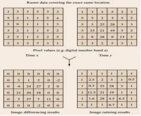
There are two main approaches to remote sensing change detection: Pixel-based and Object-oriented. Pixel-based performs change detection on only the spectral properties of corresponding pixels from imagery of the same area at different times whereas object-oriented takes into consideration the surrounding environment of the pixel as well. Figure 5 shows the main techniques used for both approaches, although there was been great advances in object-oriented techniques, the most widely used methods are image differencing and ratioing due to
Change Detection
Approaches
Pixel Based
Object-Oriented
- Image differencing - Image ratioing - Regression analysis - Principle component analysis (PCA) - Post-Classification comparison
- Support vector machine (SVM)
- Objects extraction from one image to another - Two segmentation separately compared - Stacked Bi-temporal Images
its simplicity. Image differencing is applied by subtraction of images pixel by pixel and band by band between images taken in different times. Image Ratioing is also a simple mathematical calculation but instead of subtraction, it’s the ratio between the images. The simplicity of the calculation results can be seen in Figure 6, where in the differencing method no change is indicated by 0 (subtracting same pixel value) and the ratio method producing a value of 1 (dividing by same pixel value). The outcome of a pixel-based classification are square pixels while object-oriented classification produces a more realistic result that creates entities of various shapes and size. This is known as multi-resolution segmentation in which pixels are grouped into uniform image objects that occur in different sizes concurrently. Since the objects are classified based on spatial context, geometry and texture rather than just a single pixel, the object-oriented segmentation follow natural landscapes more realistically. Multiple bands with various resolutions of different formats can be incorporated in order to better execute an object-based classification. Data in different forms such as infrared, shapefiles and elevations can be coupled into an object-based image analysis simultaneously. Supervised classification is similar to the nearest neighbor (NN) classification used in object-oriented analysis that takes into consideration the vicinity relations, nearness and distance between the multiple layers which conveys context to the analysis. After the segmentation, the user provides the training data for the landcover classes on which the image object statistics are based on. Once the statistics have been defined for each landcover type, the objects are classified accordingly (Dehvari 2009).
Blundell (2006) used subsets of principal component analysis (PCA) images to perform object-based classification using the software Feature Analyst. The software considers both the spectral and spatial information of the pixel clusters through inductive learning algorithms (Blundell 2006). This improves the overall accuracy since the classifier uses the spectral information around the pixel to perform the classification as opposed to the pixel based approach that doesn’t take any spatial context into consideration and analysis is done on a single pixel (YAO 2004). When comparing pixel-based classification vs object oriented classification, Weih (2010) produced 90.95% for pixel verses 94.47% obtained for object oriented classification when applying change detection in the Nothofagus forests (classifying between four classes). The authors were successful in isolating the two species of forests from water and non-forest features. For low to medium spatial resolution imagery, where objects and the pixel size are fairly similar in scale, the classification methods have shown to have similar accuracy. When high spatial resolution imagery is available, and objects consist of many pixels, that’s
where there’s a dissimilarity in accuracy between the two methods. The aforementioned study is a good example of some of the limitations of pixel-based image classification techniques (Weih Jr 2010).
2.3
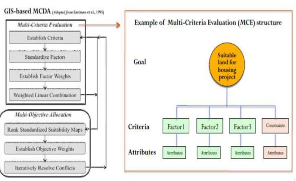
Multi-Criteria Decision Analysis (MCDA)
MCDA methods were found during the 1970s when critique arose of the traditional neoclassical environmental economics (Keeney 1976). The main weakness to the conventional neoclassical
approach when regarding environmental and economic growths is that it can’t cope effectively
with external negative spillover effects (ex. Pollution) (Nijkamp 1980). Exploration of decision problems in a more multidimensional manner that included procedural elements followed the coming years. Multidimensional approaches such as MCE provides a more comprehensive comparison between alternative choices that take into consideration environmental and socio-economic factors (Carver 1991).
1) Set goal/ define problem
i. Has to be specific and measurable within a reasonable time-bound 2) Select the criteria (factors and constraints)
i. Should be measureable and the level of detail of the data should be decided (all roads vs only major roads)
3) Normalize criteria scores
i. Have a common scale for suitability values of factors for proper comparison (fuzzy membership functions)
4) Determine factor weights
i. Rate the factors using scale between 0 to 1 against each other, total summation equals 1 (lowest number = least important, highest number = most important, pairwise comparison) 5) Aggregate all criteria
i. Weighted linear combination is used to formulate the decision rule, as follows: * All factors are combined into linear formula to produce a suitability map
6) Validate
i. Compare with ground truth or reference data to test for reliability of the results
3
STUDY AREA AND DATA
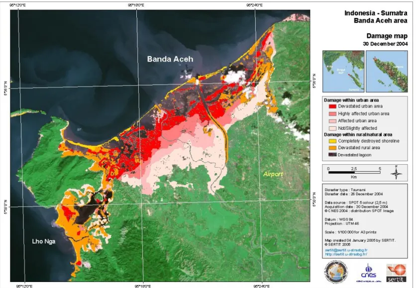
On December 26, 2004, an earthquake with a magnitude of 8.9 occured to the west of Sumatra Island of Indonesia. The earthquake in the middle of the ocean (tsunami) caused tidal waves up to 30m that struck twelve countries within the Indian Ocean. The 2004 tsunami was estimated to have released 1.1x10¹⁷ joules of energy which is equivalent to 26 megatons of TNT or 1,500 times the energy created by the Hiroshima atomic bomb (USGS 2010). Figure 8 shows the epicenter of the tsunami and the countries that suffered loss of lives and endured extreme damage, particularly settlements along the coast. The tsunami was one the most deadly disasters recorded in recent times with an estimated total damage of 15 billion dollars and over 300,000 people either missing or found dead (Matsumaru 2012).
The Study Area is Banda Aceh, Indonesia situated north-western tip of Sumatra Island at the mouth of the Aceh River (Figure 9). It is an important transportation and trading hub in the Eastern Indian Ocean with a population of 220,000. The city covers an area of 65km2 and is
home to many important landmarks for the Acehnese people of Indonesia. The 2004 tsunami
with tidal waves of up to 30m destroyed the whole city with total destruction of all infrastructure within 2 km of the coast.
3.1
Data
Two Landsat 5 satellite images around the disaster date of December 26, 2004 were downloaded from EarthExplorer (http://earthexplorer.usgs.gov). The images had some cloud
cover to the northeast of Banda Aceh which was masked out and wasn’t used for analysis. Table
1 below, provides further information on the images used.
Acquisition Date Sensor Path/Row Landsat
Number of bands
Radiometric Resolution
21/12/2004 TM 131/56 5 7 8 bits
22/01/2005 TM 131/56 5 7 8 bits
Table 1- Landsat 5 Satellite Imagery Properties
Open Street Map (OSM) data was also downloaded from geofabrik (http://www.geofabrik.de/) for Indonesia.
3.1.1
Reference Disaster Map
The International Charter’s SERTIT agency produced damage assessment maps of Banda Aceh three days after the tsunami occurred (Figure 10). As part of the rapid mapping initiative, SERTIT failed to produce a damage map within the 12 hour set goal. SERTIT used Spot imagery with 2.5 meter spatial resolution and ground data to produce this damage map characterized into two groups, damage within urban areas and damage within rural/natural area. The damage is quantified into four groups from total devastation to no/slight damage. This map will be used as the reference map to compare with the maps produced. Although this map is meaningful and easy to understand for non-GIS users, the three days it took for processing is concerning given the context of the disaster event. Right after a disaster event hits, time is of essence in order for maximize the human recovery phase. The field, local authorities can greatly benefit from a rapid generalized analysis that will provide an overview of the affected area
similar to SERTIT’s map to efficiently and effectively allocate emergency efforts within a short
3.1.2
Reference Temporary Living Centres (TLC)
There wasn’t any reference data to evaluate the generated temporary housing center sites quantitatively. A UN map of temporary living sites after the 2004 tsunami in Banda Aceh can be seen in Figure 11. The map shows that most of the temporary living sites within Banda Aceh are located around the outskirts of the city with very high concentration on the south-eastern and north-western. Visual analysis will be conducted between the relative locations of the temporary living sites in the map and the ones obtained from MCDA to test if the factors chosen and the weights given were reasonable.
4
METHODOLOGY
The semi-automated workflow for creating disaster maps and temporary housing sites is illustrated in Figure 12. Image differencing and ratioing change detection is applied to pre and post disaster Landsat 5 TM satellite images based on city blocks created from the road network. Geometric classification is then applied to classify all the resulting change detection calculations into four classes and then compared against the SERTIT reference map. Error confusion matrix is then used to evaluate the overall and kappa accuracies. The most accurate map is then used with OSM data to compute Multi-Criteria Analysis in selecting the most suitable temporary housing sites for displaced individuals.
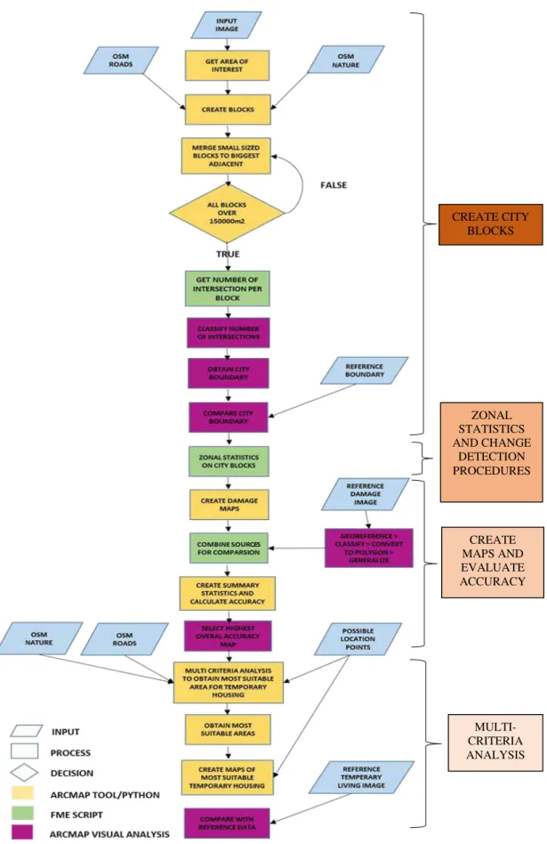
The semi-automated workflow consists of eight tools that follow a sequence with vital visual analysis steps in between some processes. Ideally, the whole workflow was planned to be implemented in Feature Manipulation Engine (FME), since the geoprocessing speed is faster than ArcMap, but due to the fact that ArcMap already has some predefined tools that perform some essential geoprocessing steps of the workflow as well as a better interface for visual analysis, it was decided to incorporate it into the workflow. The workflow requires the use of both ArcMap’s Modelbuilder and Python capabilities as well as FME’s visual scripting. This is due to the fact that both applications have their strengths and weakness, where ArcMap has specific tools for some processes as well as better visualization and FME is more efficient and powerful with regards to complex processes especially when dealing with big data. One of the goals of creating this workflow was to minimize the time required to create the damage assessment maps by means of incorporating the use of both the applications. Overall, ArcMap is used to create five tools and all visual analysis of results is done within ArcMap, and three tools are created in FME. The workflow is broken up into four main parts:
1. Creation of blocks
2. Zonal statistics and change detection procedures 3. Map creation and accuracy evaluation
4. Multi-criteria analysis
The workflow was designed to offer accurate damage results within a short time frame in order to maximize emergency response efforts. The workflow makes two assumptions for detecting change:
1. The extent of change in a pixel value from pre to post imagery is correlated with damage disregarding other factors that may have influence
CREATE CITY BLOCKS
ZONAL STATISTICS AND CHANGE
DETECTION PROCEDURES
CREATE MAPS AND EVALUATE ACCURACY
MULTI-CRITERIA ANALYSIS
4.1
Pre-Processing
4.1.1
Image
Usually geometric, radiometric and atmospheric corrections are applied when performing change detection on multi-date imagery. Geometric and atmosphere corrections were ignored due to the fact that area of study was cloud free and the Landsat imagery was already geometrically corrected. Radiometric correction is crucial for change detection analysis as it adjusts for the difference in atmospheric and sun geometry conditions. When the time between the images is minimal and taken in the same season, sometimes radiometric corrections can be ignored because the change is minimal. Song (2001) argued that radiometric correction isn’t needed when using maximum likelihood classifier or post classification on a single date or on classification of multi-date composite imagery that is placed into a single dataset. A quick test using linear normalization was applied and the difference between the normalization values and the true digital number was minimal, so it was decided to ignore applying the correction. Overlooking all the corrections and working with the raw image simplifies the workflow and quickens the process which can be indispensable for rapid mapping of an area affected by a disaster.
The Landsat image was clipped to Banda Aceh and the surrounding areas. Figure 13 shows an area of around 70km2 being clipped from the original Landsat imagery. The goal was to assess
the damage of Banda Aceh so all the other more natural surrounding areas were clipped out.
4.1.2
Open Street Map Data
OSM data was downloaded for Indonesia and clipped to the same extent of the image. The features used from the OSM dataset are as follows: OSM roads (linear), OSM nature (polygons) and OSM buildings (polygons). The OSM nature was filtered to only keep: Forests, parks, and water bodies (Ocean and River). The OSM building file was also filtered to only keep buildings that were easily accessible/recognisable and large enough to accommodate a relatively large number of people: Hospitals, school, mosque, church, place of worship, police station. The area for the OSM buildings were then calculated and the polygons converted to points. The OSM data was also cleaned to account for inconsistent naming of some feature types and to diminish the effects of noise and redundant data.
4.2
City Block Creation from Roads
ArcMap is used for the first phase of the workflow which leads to the development of the city blocks. The artificial city blocks are created from the road network and the OSM nature file is firstly used to create the coastline and disregard everything inside water as well as delete from the resulting polygons areas that are occupied by forests and parks because the main goal of the study is to evaluate urban built-up damage.
In the area of study, the OSM roads were classified as mostly residential (approximately 90%), so the roads weren’t filtered before the creation of the blocks since the blocks would have been too large due to the loss of the network if the residential roads were to be taken out. With the residential roads included, many small irrelevant blocks will be created that at a small scale
map such as the one that will be produced by this research will only add the “salt and pepper”
effect which will make it harder to visually analyse patterns and locations of damage.
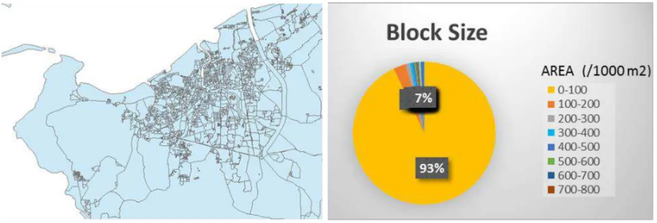
Figure 15 – First Iteration of City Blocks and Block Areas
Figure 15 shows the blocks created (left) and the size of each block. The majority of the blocks (about 93%) are under 100,000 m2, indicating that most of the blocks are insignificant to the
“big picture” or overall pattern and will only add uncertainly when visually inspecting the map. Through descriptive analysis coupled with visual analysis of the blocks, it was decided to merge all blocks under 150,000m2 to the largest adjacent polygon. Since some of the small polygons
(under 150,000m2) are surrounded by small blocks, the process had to iterate five times in order
to ensure every block was over 150,000m2.
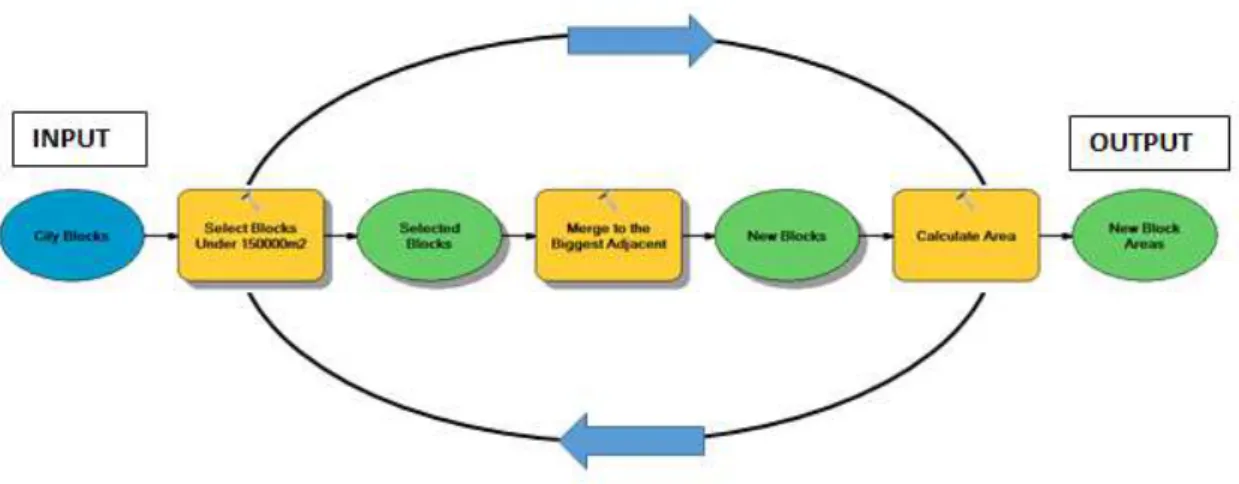
The iteration is done in a python script within ArcMap, in which a while loop is used to run through the block size and execute the merge of blocks under 150,000m2 to the largest adjacent
until all blocks are over 150,000 m2. The logic of the python script can be seen in Figure 16 in
which three ArcMap tools are used to run the merging of blocks. The city blocks are introduced as the input, firstly each block with an area of under 150,000m2 is selected using the select layer
by attribute tool. Once the blocks under 150,000m2 are selected, then the selected blocks are
merged to the remaining blocks to form larger blocks. Then the block areas are calculated again, and the process is ran again until the count of the selection of blocks is 0. For this dataset, the script iterated five times in order to achieve polygons of over 150,000m2.
Figure 16 – The Block Size Iteration Workflow
The new city blocks created by the roads nature file can be seen in Figure 17. The size of the blocks are more uniform in around the city with larger blocks in the surroundings. The most prominent block size is between 150,000 to 250,000m2. The city block area are also more even
with over 75% of the blocks falling between 150,000 to 750,000m2. The average size is just
under 500,000m2, with most of the blocks having areas around that mark. There are a few really
exceptionally large polygons usually in the surrounding rural area, which will be eliminated from the study once only the polygons corresponding to the inner core (urban built-up) of Band Aceh are selected. The city block size are now ready for further analysis but first the city boundary of Banda Aceh needs to be obtained. One can assume that larger polygons are not part of the city limits due to the lack of roads infrastructure. To obtain the city limit and use only the blocks that fall within the city limit, the road network was used as a basis for delineation. The road network was clipped for each city block so that only the roads within each block was obtained. The number of intersections is then counted by creating a point at each intersection using the intersector transformer in FME. The point on area transformer is then used to group the points per block. Since some blocks are larger in size than others, using only the count of intersection won’t be a reasonable indication for urban development. The number of intersection points is divided by the area to get a density value, which provides a better means of comparison. A new field is created with the density values for each block using the attribute creator transformer in FME. A new shapefile is created with the addition density field and the script workflow can be seen in Figure 18 as well as the tool interface.
The shapefile is then added to ArcMap where it is classified automatically into three classes using geometric classification. The resulting classified map can be seen in Figure 19, where two classes seem to be closely related to road density and the third class just being the surroundings. Adding the road network on top of the classified map clearly shows the pattern
that seems to show the city boundary. The blocks within the two classes is then extracted and used as the city boundary. The city boundary is then tested against the satellite image of the pre event image and the outcome follows the boundary for the most part. This semi-automatic method for city boundary is used instead of post-classification because it requires less insight on the user part and it can be automated, whereas post-classification method of classifying urban areas from other classes will require training sites as well as post-classification analysis. Limiting the analysis to only the blocks within the city limits will reduce the influence of the other insignificant surrounding blocks into calculating the change statistics for disaster assessment.
4.3
Zonal Statistics and Change Detection
The city blocks are then used to run zonal statistics for the pre and post disaster images with change detection computed using two different approaches: image differencing and image ratioing. For change detection, image differencing and ratioing are the two most commonly used, simplest, efficient and most effective in terms of accuracy. Singh (1989) evaluated the most common change detection techniques in forest change. The simple techniques such as image differencing and ratioing out performed much more sophisticated methods such as principal components analysis (PCA).
A script in FME is implemented to calculate and organize all the zonal statistics for both images as well as calculating the differencing and ratio values between the images (Figure 20). FME
The script can be broken down into three parts, with the first part seen in Figure 21, deals with the creation of the indexes, clipping the image to the boundary of the city limits and finally converting the information of each pixel into a point feature. Data is dealt with more efficiently and easier in FME using point features rather than raster data especially when doing zonal statistics manipulations. Every process is run twice, once for the pre-event image and the other for the post-event image in order to do the comparison and analysis at a later stage. The only requirements for this script are the pre and post image of the area and the city blocks. In this part of the script, eight raster files are created which comprises the four indices for each image. The information of the raster is also clipped to the area of interest and converted to points for further manipulations.
The points now contain the values for each band, and using the statistics calculator, the corresponding bands are subtracted and divided for each point and then sorted by block (Figure 22). A DBF file is created, that includes all the raw data regarding the differencing and ratioing values of all the bands and indices for the following statistics: max, min, range, mean and standard deviation. The by-product DBF file contains all the raw data for validation purposes. All the final values can be traced back to the DBF to check for consistency. Two DBF files are created, one for differencing and other for ratio results containing 110 columns: 10 for each band/index and 5 columns for each corresponding before and after disaster image of which 5 columns relates to the maximum value, minimum value, range, mean and standard deviation for each block. Each block contains zonal statistics that will be used to compute change detection.
In this part of the script, the statistics for before and after images are subtracted or divided to calculate the change variable for each block using the expression evaluator in FME. It was decided to apply the change detection methods on only the mean and standard deviation because it provided the most meaningful information about the blocks. Again another DBF file is created to verify all the fields were computed correctly and for consistency. The calculations are sorted by the block ID using the sorter tool in FME. The final product of the FME tool is a shapefile of the city blocks with added information on mean and standard deviation for each band/index. The different fields of the new shapefile can be seen in Figure 23, indicated by the green arrows. The values of the reference damage map by block that will be used to evaluate the accuracy is also added to the file using the feature merger. The shapefile is now ready to be classified for damage.
Figure 22 - FME Script for Change Detection Calculation – Part 2
4.4
Map Creation
The map creation was done in ArcMap using the reclassify tool in which geometric interval classification was applied independently on all band/indices change values with the purpose of obtaining four classes. The reason it’s decided to have four classes of damage is to have direct comparison of results against the reference map which also had four levels of damage (Figure 10). Geometric classification was introduced by ESRI Geostatistical Analyst extension and is useful for visualizing not normally distributed continuous data. This method is designed for data that contains many duplicate values. Since the descriptive analysis showed the data not being normally distributed and having many identical values, it was decided to use this method for automatic classification. A vital step is setting the threshold boundaries for change vs no change which can alter the results considerably. It requires understanding the data and manual intervention and due to this being a semi-automated workflow, the threshold was automatically selected by the geometric classifier which may not guarantee the optimal result. Each of the blocks will be allocated into one of the automatically generated class based of the change values calculated in the previous step. The class with the highest change will correspond to the extreme damage and the lowest to no change will be assumed to be low damage. With eleven fields to map for each method (differencing and ratioing) plus the two statistics measures (mean and standard deviation), overall 44 maps were created to be evaluated with the reference map for accuracy. Figure 24 shows maps created from differencing of the six Landsat bands. The darker blue indicates more damaged blocks than lighter shades and the general trend makes sense indicating that the more damaged blocks are closer to the ocean except for the shortwave infrared maps which show random patterns.
4.5
Multi-Criteria Decision Analysis
Safe land is a scarce resource during a disaster, so the selection for the best temporary housing site has to take many things into consideration. Decision making of how the land should be
used is not an easy task as a result of people’s different priorities, goals, interests and concerns. Spatial decision problems usually have many alternative solutions which at times are in conflict with each other. Since many possible options and criteria are evaluated by many individuals,
it’s only expected that the preferences and objective ranking of many are inconsistent. GIS-based Multi-Criteria Decision Analysis (MCDA) is an effective tool in aiding the decision making process between alternatives. MCDA provides the mechanism for configuring decision problems by evaluating alternatives to essentially rank and prioritise them. Combined with GIS data this adds a spatial component that can principally help decision makers make better and more informed decisions.
The pair-wise comparison method was implemented with the aim of obtaining the weights of importance for each factor. To diminish the effects of biases, the importance of each factor against another factor was evaluated by three experts and normalized to 1 (100%). The normalized percentage of importance for each factor by the three experts can be seen in Table 2. All three experts had the same census with different variations, with the damage map being the most important and building size being the least important among the factors. Then the average of all three experts were calculated and the final weights were obtained for the linear combination formula to aggregate all the criterias. The damage map will have the most importance with 50% followed by the proximity to roads and water (20%) with building size being the least important (10%) Experts are defined as individuals with over five years of experience in the domain of GIS.
Damage Map
Proximity to
Water Proximity to Roads
Building Type & Size
Expert 1 40 25 25 10
Expert 2 45 25 15 15
Expert 3 65 10 20 5
FEATURE WEIGHT (%)
Damage Map 50
Proximity to Water 20
Proximity to Roads 20
Building Type &
Size 10
The MCDA tool was created in ArcMap and the workflow is shown in Figure 26. For the roads and water the distance is calculated first then reclassified into ten classes. After all the factors are reclassified the weighted overlay is used to signify the importance of each factor and by weighted linear combination, a suitability map is created (Figure 27). Then the highest suitable areas (suitability of 9 and 10) are towards the south of Banda Aceh away from the ocean and extreme damage areas. The highest suitable areas are selected and the building points within the suitable areas are chosen as the most suitable for temporary living sites for displaced individuals.
The tool interface is shown in Figure 28 below.
Figure 27 – Suitability Map for Temporary Living Centre created by MCA
4.6
Accuracy Assessment
4.6.1
City Boundary
The city boundary created from road intersection density is assessed using two methods. The city boundary is a critical step because it selects the blocks within to apply change detection, therefore ensuring its acceptable is vital. Firstly, visual analysis on the city boundary overlaying the pre-event image is undertaken to assess if the city follows the urban outline of Banda Aceh. Figure 29(a) shows the city boundary on the pre disaster image, the outline appears to follow the urban areas of Banda Aceh generally well with some natural areas surrounding the south and northern side. This can be attributed to the fact that the blocks are artificially derived from the roads: where there are fewer roads (outskirts of the city), the blocks tend to be larger and less accurate.
(a) (b)
(c) (d)
The acquired city boundary is compared against the administrative boundary of Banda Aceh from 2014. Figure 29(b) shows that the administrative boundary covers about 26% more area than the acquired boundary from road density. Figure 29(c) shows the two boundaries against 2004 imagery which shows that the road city boundary follows the urban areas (indicated by colours other than shades of green) more closely. The areas highlighted by red circles are areas of most variation between the two boundaries, but one can visually observe that urban development is minimal in those areas. Figure 29(d) shows the boundaries with the roads also overlaid, which again shows that there’s no indication of urban development in the extra areas included in the administrative boundary demonstrated by the low density of roads in the highlighted areas. The disparity between the two boundaries can be attributed to two key factors. Firstly the administrative boundaries include surrounding green areas and not only the densely populated areas. Secondly Banda Aceh had a population of 219,070 people in 2000 compared to 235,245 people in 2014 which is almost a 10% increase. The possibility of the city expanding in the surrounding areas of Banda Aceh is high. The city also received 7 billion dollars of aid from over 700 domestic and international organizations which could have also led to many urban development projects around the inner core of Banda Aceh to accommodate the increasing population. Due to the factors discussed above, the city boundary derived from
road density was used as it provided a better outline of the urban areas of Banda Aceh.
4.6.2
Disaster Maps
Overall, 44 disaster maps are produced using six Landsat 5 TM bands and specific indices that highlight vegetation, water and built-up areas. The maps produced show different patterns depending on the band/index used and the method of change detection applied so it is essential to evaluate the results with the aim to observe the best band/index for mapping urban damage from the 2004 tsunami occurring in Banda Aceh and to conclude which method is better for change detection. SERTIT, a rapid mapping agency operating under the International Charter initiative produced a damage assessment map using SPOT imagery three days after the disaster occurred. The product is a map in JPEG format so for it to be used as a reference map for direct comparison, it had to be georeferenced and rectified to the imagery. The reference image is clipped to the area of interest and six control points are used to georeference the reference image