Spectral Derivation of the Ornstein-Zernike Decay
for Four-Point Functions
F. Auil and J. C. A. Barata
Universidade de S˜ao Paulo, Instituto de F´ısica and S˜ao Paulo, SP 05315-970, Brazil
Received on 10 December, 2004
In this note we discuss the relation between the Ornstein-Zernike decay of certain four-point functions (“energy-energy correlations”) in lattice spin systems and spectral properties of the transfer matrix, related to the property of two-particle asymptotic completeness in (massive) Euclidean lattice quantum field theories.
I. INTRODUCTION
In Statistical Mechanics, power-law corrections to the ex-ponential decay provide an improved asymptotic description for two-point functions (or pair-correlation) away from the critical point. Such corrections have been analysed since the pioneering work of Ornstein and Zernike [1] and its nature has been associated to other underlying phenomena.
In this paper we study the Ornstein-Zernike (O-Z) behavior of four-point functions in the context of (massive) Euclidean quantum field theories on thed+1 dimensional integer lat-tice or, correspondingly, in the context of classical statistical mechanics spin systems described by the transfer matrix for-malism. We follow closely the methods of Paes-Leme [9]. More precisely, our work attempts to extend that results to four-point functions and for the case of absolutely continu-ous energy-momentum spectrum. Therefore, the emphasis of the present work is to associate the O-Z corrections to spec-tral properties of the transfer matrix related to the absence of two-particle states and to properties of the dispersion curve of one-particle states near the origin.
Our main result is expression (III.6) in Theorem III.1 below. For the specific case of the Ising model at high temperatures in space dimensiond=1 or 2, our expression (III.6) is weaker than the known bound (obtained by more specific methods. See, e.g., [15]), while for d >3 we are able to reproduce the bound known for that particular model (see [15]). In this context, it is opportune to remark that our results and meth-ods are based on general hypotheses, valid in essentially any model described by the transfer matrix formalism and with-out two-particle bound states, as we discuss in Sec. VI. In fact, the exact asymptotics ind=1 or 2 for the Ising model at high temperatures are, in the framework of this paper, due to of additional model-dependent properties of the functionvin (III.5). See Sec. VII for some comments on this in our context or [15].
Rather than providing a replacement to other well-known methods employed in Statistical Mechanics for the analysis of decay properties ofn-point functions, as random walk meth-ods, our aim is to illuminate, in a model independent way, the relation between O-Z corrections and spectral properties asso-ciated to the particle structure of certain statistical mechanics systems, seen as lattice quantum field theory models through the transfer matrix formalism. Random walk methods may not be available in models exhibiting continuous symmetries, while our spectral hypotheses could in principle be verified
even in such cases by other formalisms, like those employed in [17, 18, 20], that use ideas originated in [23].
To emphasise the features of our spectral approach, let us present a brief historical review of the O-Z properties. The original argument of Ornstein and Zernike consists basically on a local limit type computation based on suitable assump-tions on the structure of correlaassump-tions. In a technical sense, this description is valid (for classical systems) in the limit of infi-nitely weak long-range potentials [2]. Fisher [3] introduced a heuristic development of these results based on a Bethe-Salpeter (B-S) type expressionGb=Cb+ρ−1CbGbfor the Fourier transform of the pair-correlationG. Here, the “B-S kernel” is given by minus the inverse of the (mean) densityρ, the “free resolvent” is the so called “direct correlation function”Cand, in this perhaps somewhat vague analogy, the critical point is identified, in some sense, with a “pole” of the “resolvent”G. Supported on symmetry arguments, the functionCis assumed to be quadratic near the origin (see [4]).
In more recent studies (see, e.g. [5–7]) the presence of power-law corrections to the exponential decay (O-Z correc-tions) has been established by the use of convergent expan-sion methods, like polymer and cluster expanexpan-sions or random walks. In the work of Campanino, Ioffe and Velenik [8], for instance, a refined expansion method was employed to de-rived a precise O-Z asymptotic formula for the decay of the two-point function, valid for all the region above the critical temperature in a wide class of finite range Ising type models.
A general spectral approach for two-point functions in the context of lattice spin systems, described by transfer ma-trices, and satisfying conditions required by lattice quantum field theories, can be found in the work of Paes-Leme [9]. There, the presence of O-Z corrections was associated to spec-tral properties of the transfer matrix related to the presence of a one-particle state and to properties of its dispersion curve near the origin (zero momentum).
[15].
Our starting point is an explicit expression (eq. (III.5), below) for the Fourier transform of the connected part of a truncated four-point function. Assuming a “local mini-mum (quadratic) behavior” for the dispersion curve at the ori-gin, we can use, as in [9], a multidimensional adaptation of Laplace method [16] for the asymptotic estimation of some integrals and, in this way, we get the O-Z decay property, namely a power-law correction as|τ0|−d,τ0being the “time”-component of the coordinateτ, defined in (III.3).
The main difference with respect to [9] is that our expres-sion (III.5) is basically a paraphrase of the two-particle as-ymptotic completeness condition studied in [19], as we will remark in Sec. VI. Roughly speaking, this represents the ab-sence of (two-particle) bound states. In a mathematical sense, the energy-momentum spectrum up 2mis, in this case, ab-solutely continuous and has multiplicity 1. Asymptotic com-pleteness is verified under general hypotheses, as discussed in [19]. The Ising model at high temperatures, for instance, matches this condition [20].
Analogous results could be derived assuming the existence of two-particle bound states but, in this case, it seems plau-sible to expect that the exponential decay is corrected by |τ0|−d/2, as in the case of the two-point function [9], instead of|τ0|−d. See the final digression of Sec. IV and Sec. VII.
Our results provide a one-way proof that some suitable as-sumptions on the energy-momentum spectrum, related to two-particle asymptotic completeness, imply a definite O-Z decay. One would be naturally tempted to speculate on the opposite direction, and ask whether the knowledge of the O-Z decay of correlations provides information on the energy-momentum spectrum which could be interpreted in terms of properties of the particle states, such as asymptotic completeness. Unfortu-nately, however, to address such interesting general questions is beyond our present capabilities, and we leave this point without further comments.
This paper is organised as follows. In Sec. II we present the basic setting we will work with. In Sec. III we introduce the basic assumptions and state our main result, captured in The-orem III.1. In Sec. IV we present some preparatory results to the proof of Theorem III.1, finally presented in Sec. V. In Sec. VI we derive the expression (III.5) under suitable hypotheses. Sec. VII is devoted to some final remarks.
II. BASIC HYPOTHESES
A model in lattice quantum field theory is specified by the choice of a state µ (i.e., a linear, positive functional with norm 1) on the algebraC³SZd+1´ of complex-valued, continuous functions on the set of configurations SZd+1 :=
©
ϕ:Zd+1→Sª, with the product topology, where S⊆Cis a conveniently topologized set. For instance, for the Ising Model we haveS:={−1,1}with the discrete topology, but restrictions onSand its topology are not really serious neither relevant in the present context. As usual,Zd+1is the lattice of
integers ind+1 dimensions, withd>1, whose sites will be
denoted byx= (x0,x1, . . . ,xd)or(x0,x), for short.
Examples of functions inSZd+1 are the projections at site x, ϕx:ϕ7−→ϕ(x), and the function identically equal to 1, denoted here by 1. For each i∈ {0, 1, . . . , d} and a∈
Z we define the semi-spaces Λi,a := {(x0, x1, . . . , xd)∈ Zd+1 : x
i>a}. We also define the lattice translations: τx: y7−→y+x, ∀x, y∈Zd+1, and the reflections θi,a:y7−→ (y0, y1, . . . ,yi−1,2a−yi,yi+1, . . . ,yd),a∈Z/2. An exam-ple is the “time” reflectionθ:= θ0,0:(x0, x)7−→(−x0, x). The stateµis interpreted as the vacuum state and is typically obtained as the thermodynamic limit of finite volume Gibbs states. Additionally, the stateµis assumed to satisfy
A1 Invariance under reflections and translations: µ = µ◦θi,a=µ◦τx, ∀i∈ {1, . . . ,d}, ∀x∈Zd+1and ∀a∈ Z/2.
A2 Reflection positivity: µ¡θ0,af f ¢
>0, ∀f ∈
P
(Λ0,a) and ∀a∈Z/2.Above, the bar indicates complex conjugation and
P
(Λ) de-notes the algebra generated by all the projections ϕx with x∈Λ. The last two properties allow to construct the Hilbert space of physical statesH
as the completion of the quotientP
(Λ0,0)/{f : hf, fi0=0}, a procedure similar to the GNS construction for C∗-algebras. Note that hf, gi0:=µ¡θf g¢ is a sesquilinear, Hermitian, non-negative form (by A2) onP
(Λ0,0). The standard procedure gives additionally acanoni-cal inclusioni:
P
(Λ0,0)→H
with dense image. For instance,i(1) =:Ωis the vacuum state vector. Functions f ∈
P
(Λ0,0)act as multiplication operators on
P
(Λ0,0), fe:g7−→ f g. Theaction of functions and the lattice translations can also be ex-tended through i, leading to operators acting on
H
. Some relevant examples are:i(ϕex) =: Φ(x), the local fields, forx∈Λ0,0,
i(τe0) =: T, the transfer matrix,
i(τen) =: Tn, the generators of space translations,
forn=1, . . . ,d.
The local fields are bounded operators if S is a compact set, withkΦ(x)k6sup{|s| :s∈S}. The transfer matrix is a positive self-adjoint operator with norm equal to 1 and the op-eratorsTn, the generators of elementary space translations on the lattice, are unitaries, so they can be expressed asTn=eiPn for certain self-adjoint operatorsPn, with spectrum in(−π,π]. We can identify P= (P1, . . . , Pd)with the momentum op-erator. The Hamilton operator is defined on Ker(T)⊥ by H:=−ln(T↾Ker(T)⊥). Notice, however, that Ker(T) ={0} in many of the most interesting models (see [21]) and, hence, Hwill be defined on the whole Hilbert space. Thus,(H,P) will be called the energy-momentum operator.
Finally, for functions f on the lattice, the Fourier transform bf and anti-transform fˇ are de-fined by bf(p) = (2π)−d+12
∑
x∈Zd+1
e−i p·xf(x) and ˇ
f(x) = (2π)−d+12
Z
Td+1
ei x·pf(p)d p, respectively. Above,
III. THE MAIN RESULT
Then-point Euclidean, or Schwinger, functions are defined by
S
n(x1, . . . , xn) := µ(ϕx1· · ·ϕxn). As a consequence oftranslation invariance A1, we can express
S
nin terms of dif-ference variablesS
n(x1, . . . ,xn) = Sn(x1−xn, . . . ,xn−1−xn). (III.1) We define the connected part of the truncated four-point func-tion asD
(x1,x2,x3,x4) :=S
4(x1,x2,x3,x4)−
S
2(x1,x2)S
2(x3,x4). (III.2)In terms of the new variables
ξ := x1−x2, η := x3−x4, τ := x1+x2−(x3+x4), (III.3) and expressing the two-point and four-point functions in terms of difference variables (III.1), we get
D
(x1,x2,x3,x4) = S4µ
τ+ξ+η
2 ,
τ−ξ+η
2 ,η
−S2(ξ)S2(η) =: D(τ,ξ,η). (III.4)
The change of variables (III.3) requires certain care in the lattice context. This was discussed in [19], and here we omit these considerations. DenoteR(k, p,q):=Db(k, p, q), considering it as a family of integral operators[R(k)f](p) =
R
Td+1R(k,p,q)f(q)dqindexed byk.
Our results on the four-point function will be obtained from the following single assumption, which we will derive from other more basic ones in Sec. VI.
a. Assumption: For each fin a “suitable” space of func-tions
A
(see Sec. VI), we havehf,R(k)fiL2(Td+1) =
Z
Td
sinhG(p, k) coshG(p,k)−cosk0
v(p,k)dp+B(k)(f), (III.5)
where
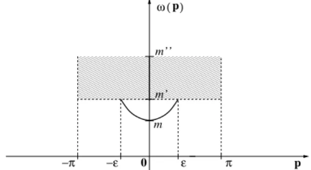
(a) G(p, k) = [ω(p+k) +ω(p−k)]/2. Here, ω is is a “sufficiently differentiable”, real function defined in the torus Td (i.e., periodic), with m :=ω(0)6ω(k),
(gradω)(0) =0, and such that the matrixB, whose
en-tries are given by
Bi j = ∂2ω
∂ki∂kj ¯ ¯ ¯ ¯k=
0
,
is positive defined and non-singular. Furthermore, there
existsm′>msuch thatm′6ω(k)for allkoutside a neighborhood of the origin. See Fig. 1.
(b) v(p,k)is a non-negative,C∞function.
(c) B(k)(f)is analytic in the strip|Imk0|<m′′, wherem′′> m′>m.
By abuse of notation, we denote the mapk07−→ hf, R(k)fi byRandD=Rˇ.
We are now in position to state our main result:
Theorem III.1 Under the assumptions above, we have
D(τ) = const e −m|τ0|
|τ0|d +e
−m|τ0|O∗ ³
|τ0|−(d+12) ´
+O
³
e−m′′′|τ0| ´
(III.6)
for τ0 → ∞, where m′′′ > m. Here, O∗(K−p) means O¡K−p+δ¢for allδ>0when K→∞. ✷
Remarks. 1.The precise meaning of expression (III.6) is the following: there existsI(τ)such that
0000000000000000000 0000000000000000000 0000000000000000000 0000000000000000000 0000000000000000000 0000000000000000000 0000000000000000000 0000000000000000000 0000000000000000000 0000000000000000000 0000000000000000000 0000000000000000000 0000000000000000000
1111111111111111111 1111111111111111111 1111111111111111111 1111111111111111111 1111111111111111111 1111111111111111111 1111111111111111111 1111111111111111111 1111111111111111111 1111111111111111111 1111111111111111111 1111111111111111111 1111111111111111111
−π π
m’’
m’
p 0
ω (p)
ε −ε
m
FIG. 1: The assumed shape of the functionωnear the origin.
wherem′′′>m, and the expressionI(τ)satisfies:
¯ ¯ ¯ ¯
¯I(τ)−const
e−m|τ0|
|τ0|d
¯ ¯ ¯ ¯
¯ 6 const
e−m|τ0|
|τ0|d+12−δ
(III.8)
asτ0→∞, for anyδ>0. The functionI(τ)is the Fourier anti-transform of the first term at the r.h.s. in (III.5). See (IV.1) in Section IV below. 2. Our derivation of (III.6) from assump-tion (III.5) is valid in anyspace dimensiond. As shown in Sec. VI, for the cased =1 we derive relation (III.5) under
some suitable hypotheses, among them the existence of a one-particle shell. In this case, the functionω of condition (a) becomes the dispersion curve of the particle andmits mass.
3. From definition (III.3), note that theτcoordinate istwice the difference between the “center of mass coordinates” (of pointsx1 andx2 and pointsx3 andx4, respectively), so the mass rate of the exponential decay in (III.6) is 2m, the ex-pected one for that particular four-point function (compare, f.i., with [23, 24]). 4. The condition on differentiability ofω
is not a physically restrictive condition. As will become clear from our proof of Theorem III.1 below, condition (b) is not essential and can be considerably weakened.
IV. SOME PREPARATORY REMARKS
Before we start the proof of Theorem III.1, let us make some preparatory comments on the decay properties ofD(τ). From (III.5), we have, by the analyticity ofB(k)(f)in (c),
D(τ) = Rˇ(τ) = I(τ) + O(e−m′′|τ0|), (IV.1)
whereI(τ)is the Fourier anti-transform of the first term at the r.h.s. in (III.5)
I(τ) = (2π)−d+12
Z
Td
Z
Td+1
sinhG(p,k) coshG(p,k)−cosk0
v(p, k)eiτ·kdk dp
= (2π)−d+12
Z
Td
Z
Td µZ π
−π
sinhG(p,k) coshG(p, k)−cosk0
eiτ0k0dk
0
v(p,k)eiτ·kdkdp
= (2π)1−2d
Z
Td
Z
Tde
−G(p,k)|τ0|v(p,k)eiτ·kdkdp. (IV.2)
The integral ink0(in brackets at the second line above) was easily evaluated by the method of residues, and its value is 2πe−G(p,k)|τ0|.
At this point we have to do a little digression. Let us denote by|p|thel∞norm of vectorsp= (p1, . . . , pd)∈Rd(orZd), |p|:=max{|p1|, . . . , |pd|}. Define the setId={n∈Zd : |n|61}and, for some conveniently smallε>0, consider the region
D={(p,k)∈Td×Td :∃n,
m∈Ids. t.|p+k+2πn|<ε
and
|p−k+2πm|<ε}.
Note that forn∈Idwe can write 2n=a+bwitha,b∈Idand |ai|=|bi| ∀i=1, . . . ,d. Note also that if the two relations
|p+k+2πn|<ε, |p−k+2πm|<ε (IV.3)
are simultaneously valid for somenandminId, thennand
mare not independent, because|p|<πand|k|<π. In fact, each component of the pair(n, m)admits just five possible values,(ni, mi) = (±1,0),(0, ±1 or 0). From these two ob-servations, the pair of relations (IV.3) is equivalent to
|p+k+π(a+b)|<ε, |p−k+π(a−b)|<ε, (IV.4) witha,b∈Idand|ai|=|bi|(for, just analyse each case sep-arately and note that the original 9=3×3 cases are reduced to 5, by the second observation above). Define the translation Ta,b:(p,k)7−→(p+πa,k+πb)and the
“rotation-reflection-dilatation” given by the orthogonal matrixA=¡1 1 1−1
¢
, where 1 denotes here thed×d identity matrix. Then, the pair of relations (IV.4) is equivalent to
|ATa,b(p,k)|<ε, (IV.5)
are the center and the corners of the dotted big square shown in Fig. 2, and the region D is the union of the five shaded diamond shaped sub-regions.
We split thedpdkintegral in (IV.2) in two pieces,RD+RDc. The integral onDc
isO(e−m′|τ0|), withm′>m. More delicate
is the analysis of the integral onD. It can be written as a sum of integrals on each of the regionsDa,b,
Z
Da,b
e−G(p,k)|τ0|v(p,k)eiτ·kdkdp. (IV.6)
In the integral above we perform the change of variables given by the transformationATa,b, with Jacobian determinant
(−2)d, to get
e−iπτ·b
2d
Z
|p|<ε
µZ
|k|<εe
−G◦(ATa,b)−1(p,k)|τ0|u(p,k)e−2iτ·kdk 
e2iτ·pdp, (IV.7)
whereu:=v◦(ATa,b)−1. Notice that the four regions in the
corners of the big dotted square in Fig. 2 are identified as a single one on the torus. Therefore, the regionDis actually the union of two diamond shaped regions on the torus. The proof of the Theorem III.1 will be continued from this exact point at the Sec. V below. The remaining of the present section is a digression.
Instead of condition (a) of the Assumption, consider the fol-lowing weaker one:
(a’ )G(p, k) is a “sufficiently differentiable” function de-fined in the torusTd (i.e., periodic), depending on the variables p andk just in the combinations p+k and
p−k respectively,m6G(p, k), and with the follow-ing property: there exists ε>0 such that the matrix B=B(p), whose entries are given by
Bi j = ∂ 2G
∂ki∂kj ¯ ¯ ¯ ¯
k=0
,
is positive defined and non-singular for|p|<ε. Fur-thermore,(gradkG)(p,0) =0, for|p|<ε.
As in [9], using the results of [16] the integral in brackets in (IV.7) can be estimated using the method of Laplace, which
gets the asymptotic decay
const e−m|τ0| "
1
|τ0|d/2 +O
∗³|τ0|−d+12 ´
#
. (IV.8)
The estimative in (IV.8) is valid for all regionsDa,b and is,
therefore, valid for the integral onD. The power-law correc-tion|τ0|−d/2to the exponential decay of the four-point corre-lations found above was obtained with a simple analysis, and a less restrictive condition onG. As we will show in the next section, they can be improved, leading to the stronger power-law correction|τ0|−d, mentioned in Theorem III.1.
V. PROOF OF THEOREM III.1
Assuming the condition (a) for the functionG
G(p,k) := ω(p+k) +ω(p−k)
2 , (V.1)
using (V.1) in (IV.7) we get
e−iπτ·b 2d
Z
|p|<ε
µZ
|k|<εe
−12ω(k−π(a−b))|τ0|u(p,k)e−2iτ·kdk 
e−12ω(p−π(a+b))|τ0|e2iτ·pdp
= e
−iπτ·b
2d
Z
|p|<ε
µZ
|k|<εe −1
2ω(k)|τ0|u(p,k)e−2iτ·kdk 
e−12ω(p)|τ0|e2iτ·pdp. (V.2)
Now we can use, as in [9], the results of [16, p. 148 and ff.] on a multidimensional adaptation of the method of Laplace to estimate both integrals in (V.2), one at each time, beginning with thedkintegral. We get that expression (V.2) decays
as-ymptotically as
const e −m|τ0|
|τ0|d +e
−m|τ0|O∗³|τ0|−(d+12) ´
00000000 00000000 00000000 00000000 00000000 00000000 00000000 00000000 00000000 00000000 00000000 00000000 00000000 00000000 00000000 00000000 11111111 11111111 11111111 11111111 11111111 11111111 11111111 11111111 11111111 11111111 11111111 11111111 11111111 11111111 11111111 11111111 000000000 000000000 000000000 000000000 000000000 000000000 000000000 000000000 000000000 000000000 000000000 000000000 000000000 000000000 000000000 000000000 111111111 111111111 111111111 111111111 111111111 111111111 111111111 111111111 111111111 111111111 111111111 111111111 111111111 111111111 111111111 111111111 000000000 000000000 000000000 000000000 000000000 000000000 000000000 000000000 000000000 000000000 000000000 000000000 000000000 000000000 000000000 000000000 111111111 111111111 111111111 111111111 111111111 111111111 111111111 111111111 111111111 111111111 111111111 111111111 111111111 111111111 111111111 111111111 00000000 00000000 00000000 00000000 00000000 00000000 00000000 00000000 00000000 00000000 00000000 00000000 00000000 00000000 00000000 00000000 11111111 11111111 11111111 11111111 11111111 11111111 11111111 11111111 11111111 11111111 11111111 11111111 11111111 11111111 11111111 11111111 000000000 000000000 000000000 000000000 000000000 000000000 000000000 000000000 000000000 000000000 000000000 000000000 000000000 000000000 000000000 000000000 111111111 111111111 111111111 111111111 111111111 111111111 111111111 111111111 111111111 111111111 111111111 111111111 111111111 111111111 111111111 111111111 −π π −π p k ε ε , a π
( πb)
Da,b π 0000 0000 0000 0000 0000 0000 0000 0000 0000 1111 1111 1111 1111 1111 1111 1111 1111 1111 0000 0000 0000 0000 0000 0000 0000 0000 0000 1111 1111 1111 1111 1111 1111 1111 1111 1111 0000 0000 0000 0000 0000 0000 0000 0000 0000 1111 1111 1111 1111 1111 1111 1111 1111 1111 0000 0000 0000 0000 0000 0000 0000 0000 0000 1111 1111 1111 1111 1111 1111 1111 1111 1111 00000000 00000000 00000000 00000000 00000000 00000000 00000000 00000000 00000000 00000000 00000000 00000000 00000000 00000000 00000000 00000000 11111111 11111111 11111111 11111111 11111111 11111111 11111111 11111111 11111111 11111111 11111111 11111111 11111111 11111111 11111111 11111111 −π π −π p k π a a b c d b c d
FIG. 2: Left: The five regionsDa,b. Right: The edges of the shaped regions with the same letter are identified in the torus, and the four cornered regions become just one diamond region, like the central one.
0000000000 0000000000 0000000000 0000000000 0000000000 0000000000 0000000000 0000000000 0000000000 0000000000 0000000000 0000000000 0000000000 0000000000 0000000000 0000000000 0000000000 0000000000 0000000000 0000000000 1111111111 1111111111 1111111111 1111111111 1111111111 1111111111 1111111111 1111111111 1111111111 1111111111 1111111111 1111111111 1111111111 1111111111 1111111111 1111111111 1111111111 1111111111 1111111111 1111111111 0000000000 0000000000 0000000000 0000000000 0000000000 0000000000 0000000000 0000000000 0000000000 0000000000 0000000000 0000000000 0000000000 0000000000 0000000000 0000000000 0000000000 0000000000 0000000000 0000000000 1111111111 1111111111 1111111111 1111111111 1111111111 1111111111 1111111111 1111111111 1111111111 1111111111 1111111111 1111111111 1111111111 1111111111 1111111111 1111111111 1111111111 1111111111 1111111111
111111111100000000000000000000 0000000000 0000000000 0000000000 0000000000 0000000000 0000000000 0000000000 0000000000 0000000000 0000000000 0000000000 0000000000 0000000000 0000000000 0000000000 0000000000 0000000000 0000000000 1111111111 1111111111 1111111111 1111111111 1111111111 1111111111 1111111111 1111111111 1111111111 1111111111 1111111111 1111111111 1111111111 1111111111 1111111111 1111111111 1111111111 1111111111 1111111111 1111111111 0000000000 0000000000 0000000000 0000000000 0000000000 0000000000 0000000000 0000000000 0000000000 0000000000 0000000000 0000000000 0000000000 0000000000 0000000000 0000000000 0000000000 0000000000 0000000000 0000000000 1111111111 1111111111 1111111111 1111111111 1111111111 1111111111 1111111111 1111111111 1111111111 1111111111 1111111111 1111111111 1111111111 1111111111 1111111111 1111111111 1111111111 1111111111 1111111111 1111111111 −π π −π p k , a
π πb)
π
(
Ra,b
FIG. 3: The regionR(shaded).
whenτ0→∞. See Appendix A for the details. This bound, valid on each regionDa,b, extends immediately to the integral
onD. The integral onDc
can be split into the integrals on two complementary regions,RandRc
∩Dc
, whereRis the shaded region in Fig. 3.
In each rectangular sub-regionRa,b, just one of the
inte-grals in (V.2) has an exponential decay with mass rate m/2 corrected by|τ0|−d2, while the other one has only an
exponen-tial decay with mass ratem′/2, withm′>m. Therefore, these integrals decay as
const e−m+m ′
2 |τ0|O³|τ0|−d/2´ (V.4)
As in the previous section, the integral onRc ∩Dc
has an ex-ponential decay with mass ratem′>m. Finally, collecting the pieces, we have
D(τ) = c′1e −m|τ0|
|τ0|d +e
−m|τ0|O∗³|τ0|−(d+12) ´
+ e−m+m
′
2 |τ0|O³|τ0|−d/2´ +O³e−m′|τ0|´ +O³e−m′′|τ0|´, (V.5)
c′1being a positive constant. This completes the proof of The-orem III.1.
VI. DERIVATION OF EXPRESSION (III.5)
In this section we derive condition (III.5) from more ba-sic hypotheses. The relation of the operator R(k) with the
Directly from the definitions we have
D(τ,ξ,η) = S4
µτ+ξ+η
2 ,
τ−ξ+η
2 ,η
−S2(ξ)S2(η)
= µ
³ ϕτ+ξ+η
2
ϕτ−ξ+η
2 ϕηϕ0
´
−µ¡ϕξϕ0¢µ(ϕηϕ0)
= µ
³
(ϕξϕ0−µ(ϕξϕ0)1).(1).τ−τ−ξ+η
2
(ϕηϕ0−µ(ϕηϕ0)1).(1)
´
= D¡Φ(ξ)Φ(0)−µ(ϕξϕ0)IH ¢
Ω,T
−τ−ξ2+η(Φ(η)Φ(0)−µ(ϕηϕ0)IH)Ω
E
H,
(VI.1)
where in the last equality we assumedξ0=0. Assuming now additionallyη0=0, identity (VI.1) takes the form D(τ,ξ,η) = DΘ(ξ), e−21|τ0|He−21iτ·PΘ(η)
E
H, (VI.2)
whereΘ(α):=e−12iα·P[Φ(α)Φ(0)−µ(ϕαϕ0)IH]Ω. Now, if f,g∈L2¡Td+1¢are symmetrical, with purely spatial dependence,
we have
hf,R(k)giL2(Td+1) =
Z
Td+1
Z
Td+1
b
D(k,p,q)f(p)g(q)dq d p
= (2π)1−2d
∑
τ,(0,ξ),(0,η)
e−ik·τD(τ,(0,ξ),(0,η))ˇf(−ξ)gˇ(−η)
= (2π)1−2d
∑
τ,(0,ξ),(0,η)
e−ik·τDΘ(ξ),e−12|τ0|He−12iτ·PΘ(η) E
H
ˇf(−ξ)gˇ(−η)
= (2π)1−2d
∑
τ
e−ik·τDΘ(fˇ),e−12|τ0|He−12iτ·PΘ(gˇ) E
H
= (2π)1−2d
Z ∞
0
Z
Td Ã
∑
τ0∈Ze−ik0τ0e−12|τ0|λ0 !Ã
∑
τ∈Zd
e−ik·τe−12iτ·λ !
dEλ
= (2π)d+12
Z ∞
0
Z
Td
sinh(λ0/2) cosh(λ0/2)−cosk0
δ µ
λ
2+k
¶ dEλ
= (2π)d+12
Z ∞
0
sinh(λ0/2) cosh(λ0/2)−cosk0
dE(λ0,−2k).
(VI.3)
Here, we have used (VI.2). Moreover, we denoteΘ(h):=∑xΘ(x)h(−x), or Θ(h) =
∑
x∈Zd
h(−x)e−12ix·P£Φ((0,x))Φ(0)−µ(ϕ
(0,x)ϕ0)1 ¤
Ω,
for the “two-particle states”, and we have introduced the spectral measure of the energy-momentum operatordEλ:= dΘ(fˇ),EλΘ(gˇ)®H.
Let us briefly present some definitions. Let the uncon-nected four-point function be defined as
D
0(x1,x2,x3,x4):=S
2(x1,x3)S
2(x2,x4) +S
2(x1,x4)S
2(x2,x3). As in expression (III.4), we can writeD
0in terms of the variablesξ,ηandτ, introducingD0asD
0(x1, x2,x3, x4) =:D0(τ,ξ,η). Let the “free resolvent”R0be defined asR0(k, p,q):=Db0(k, p,q), considered as a family of integral operators indexed byk. Act-ing on symmetric functions,i.e., f(p) = f(−p), it is given by R0(k,p,q) =2(2π)d+12 Sb2(k+p)Sb2(k−p)δ(p+q)(see [19]).The so-called Bethe-Salpeter kernelKis defined by the Bethe-Salpeter equationR=R0−R0KR. Now, consider the follow-ing hypotheses:
H1 Existence of “one-particle states”: The Fourier trans-form of two-point function is given by:
b
S2(p0,p) =
Z(p)sinhω(p) coshω(p)−cosp0 +
Z ∞
m+2δ0
sinhλ0 coshλ0−cosp0
whereZ(p)is a positive,C∞function;ω(p)is real ana-lytic,m6ω(p)<m+2δ0; 0<δ06m.
H2 Exponential decay of the Bethe-Salpeter kernel: The Bethe-Salpeter kernel K(k, p,q)is analytic in the re-gion
|Impi| < δi+ε(i=0,1, . . . ,d) |Imqi| < δi+ε(i=0,1, . . . ,d) |Imk0| < m+δ0
for certainδi>0 (i=1, . . . ,d), andε>0.
H3 “Repulsive interaction”: K(k, p, q) = η1 +
η2K1(k, p, q), with K
1 satisfying H2. Here 1 is the function identically equal to 1 and ηis a positive constant.
The hypotheses H1-H3 were verified in various models under several conditions by many authors (see [19] for a large list of references). We introduce also the following few definitions
δ := (δ0,δ1, . . . ,δd)∈Rd+1,
Iδ := n(α0,α1, . . . ,αd)∈Rd+1 :|αi|6δi, ∀i=0,1, . . . ,d o
,
kfk2δ := sup α∈Iδ Z
Td+1
|f(p+iα)|2d p,
Aδ := {f : f is analytic in |Impi|6δi, kfkδ<∞, f(p) =f(−p)}.
It was proven in [19] that, for f inAδ, the measuredΘ(fˇ),EλΘ(fˇ)®H vanishes in(0, 2m)and, ifd =1, has a Radon-Nykodim derivative in[2m,2(m+δ0)), given by
dΘ(fˇ),E(λ0,−2k1)Θ(fˇ)®H = 2πZ(F−1(λ0) +k1)Z(F−1(λ0)−k1)
×(F−1)′(λ0)W f W f(0,F−1(λ0))dλ0, (VI.5) where, denoting(p0,p) = (p0, p1),(k0,k) = (k0,k1)and cosk0−1=x+iy, withx,y∈R, we have
F(p1) := ω(p1+k1) +ω(p1−k1),
W f := lim
y→0+ x→θ(p)−1
[1+K(k0,k1)R0(k0,k1)]−1f,
θ(p1) :=
r
cosh[ω(p1+k1) +ω(p1−k1)] +1
2 .
Replacing expression (VI.5) in the last integral in (VI.3), after the the change of variables given byp1=F−1(λ0), we have hf,R(k)fiL2(Td+1) = (2π)
d+3 2
Z
T
sinh(F(p1)/2) cosh(F(p1)/2)−cosk0
v(p1,k1)d p1 +B(k)(f), (VI.6) where
v(p1,k1) = Z(p1+k1)Z(p1−k1)W f W f(0, p1), (VI.7) B(k)(f) = (2π)d+12
Z ∞
2(m+δ0)
sinh(λ0/2) cosh(λ0/2)−cosk0
dΘ(fˇ),EλΘ(fˇ)®H . (VI.8)
This establishes (III.5) under the above hypotheses. VII. SOME FINAL COMMENTS
As a final remark, let us point that special mechanisms, eventually occurring in some model-specific situations and possibly related to particular symmetries or low-dimensional
properties, can lead to some improvements of our estimates. Expression (III.5) reflects the fact that the spectral mea-suredE(λ0,−2k)in (VI.3) is absolutely continuous belowm′′= 2(m+δ0). Physically, this fact reflects the absence of bound states. In the presence of two-particle bound states, additional
as in the case of the two-point function, studied by Schor in [22], wherewis analogous to the dispersion curveω. In this case, a term like
sinhw(k) coshw(k)−cosk0
has to be added to the r.h.s. of (III.5). As in the Sec. IV, it is easy to prove that such a term leads to a decay as (IV.8).
In terms ofΓ, the convolution inverse of the two-point func-tion, satisfying
b
S2(p0,p)bΓ(p0,p) = −1, (VII.1) the dispersion curve ω is implicitly defined by
b
Γ(±iω(p), p) =0, while the C∞, positive function Z is defined by (see [22])
∂bΓ(p0,p)
∂(cosp0−1)
¯ ¯ ¯ ¯ ¯
p0=±iω(p)
= 1
Z(p)sinhω(p), (VII.2)
from which we get
Z(p) =
i ∂Γb(p0,p) ∂p0
¯ ¯ ¯ ¯ ¯p
0=±iω(p)
−1
. (VII.3)
By reflection invariance A1 (Sec. II), the two-point function
b
S2is a symmetric function ofp. From (VII.1),Γbis equally symmetric and, finally, by (VII.3), the functionZis symmetric as well.
Assume that the functionvin (III.5) is of the formv(p,k) = Z(p+k)Z(p−k)v1(p), withZ symmetric. From the above observations and from (VI.7), this condition is not much re-strictive. Under this hypothesis, the integral in (V.2) assumes the form
Z
|p|<ε
µZ
|k|<εe −1
2ω(k)|τ0|Z(k−2πm)e−2iτ·kdk 
e−12ω(p)|τ0|Z(p−2πn)u1(p)e2iτ·pdp. (VII.4)
By the symmetry ofZ, we have|Z(p)| ≃z1+z2|p|2near the origin, wherez1,z2are constants. Using this and the previously mentioned asymptotic estimates, expression (VII.4) becomes asymptotically
e−m|τ0| "Ã
c1 |τ0|d +
c2 |τ0|d+1
!h
1 +O∗³|τ0|−(d+12) ´i
+ c3
|τ0|d+2
#
. (VII.5)
In specific models, it can happen that the constantc1above vanishes and the leading term becomes c2e−m|τ0|/|τ0|d+1.
This behavior could also be reproduced provided the func-tion v1 above behaves as|v1(p)| ≃ |p|2 nearp=0. This is possibly what happens in the high temperature Ising model in d=2, where only thec2-term reproduces the correct asymp-totics. The precise analysis requires a model-specific study of the properties of the functions Z andv1 that are beyond the scope of our general approach. See f.i. [15]. Note that
the vanishing of eitherc1orc2is compatible with the claim c′1>0 in (V.5). The claim would be incompatible only ifboth c1and c2of (VII.5) weresimultaneouslyzero.
APPENDIX A: PROOF OF (V.3)
Considering the integral in (V.2), for anyA,B,C positive numbers we can write
B ¯ ¯ ¯ ¯em|τ0|
Z
|p|<ε
µZ
|k|<εe −1
2ω(k)|τ0|u(p,k)e−2iτ·kdk 
e−12ω(p)|τ0|e2iτ·pdp −A ¯ ¯ ¯ ¯
= B
¯ ¯ ¯ ¯ ¯e
m 2|τ0|
Z
|p|<ε
Ã
em2|τ0|
Z
|k|<εe −1
2ω(k)|τ0|u(p,k)e−2iτ·kdk − C
|τ0|d/2 + C |τ0|d/2
!
e−12ω(p)|τ0|e2iτ·pdp −A ¯ ¯ ¯ ¯ ¯
6 B ¯ ¯ ¯ ¯ ¯e
m 2|τ0|
Z
|p|<ε
Ã
em2|τ0|
Z
|k|<εe
−12ω(k)|τ0|u(p,k)e−2iτ·kdk − C
|τ0|d/2
!
e−12ω(p)|τ0|e2iτ·pdp ¯ ¯ ¯ ¯ ¯
+B
¯ ¯ ¯ ¯ ¯
C |τ0|d/2 e
m 2|τ0|
Z
|p|<εe −1
Now, as a consequence of equation (2.9.6) in [16, p. 149], we have
Z
|p|<εe
−21ω(p)|τ0|e2iτ·pdp = e− m 2|τ0|
Z
|p|<εe
−12(ω(p)−m)|τ0|e2iτ·pdp
= e−m2|τ0|
Z
|p|<εe
−14hp,Bpi |τ0|e2iτ·pdp+O∗ ³
|τ0|−d+12 ´
(A.2)
The Gaussian integral at the r.h.s. in (A.2) can be bounded by a term proportional to|τ0|−d/2. Therefore
¯ ¯ ¯ ¯ ¯e
m 2|τ0|
Z
|p|<εe −1
2ω(p)|τ0|e2iτ·pdp− C1
|τ0|d/2
¯ ¯ ¯ ¯ ¯ 6
C2 |τ0|d+12 −δ
. (A.3)
Analogously,
¯ ¯ ¯ ¯ ¯e
m 2|τ0|
Z
|k|<εe −1
2ω(k)|τ0|u(p,k)e−2iτ·kdk − C3
|τ0|d/2
¯ ¯ ¯ ¯ ¯ 6
C4 |τ0|d+12 −δ
. (A.4)
If we setA=C3C1|τ0|−d,B=|τ0|d+
1
2−2δandC=C3, using (A.3) and (A.4) the first term at the r.h.s. in (A.1) is bounded by BC4C2|τ0|−(d+1)+2δ=C4C2|τ0|−1/26C4C2, and for the second we have
B ¯ ¯ ¯ ¯ ¯
C3 |τ0|d/2e
m 2|τ0|
Z
|p|<εe
−12ω(p)|τ0|e2iτ·pdp− C3C1
|τ0|d/2|τ0|d/2
¯ ¯ ¯ ¯ ¯
6 B C3 |τ0|d/2
¯ ¯ ¯ ¯ ¯e
m 2|τ0|
Z
|p|<εe −1
2ω(p)|τ0|e2iτ·pdp − C1
|τ0|d/2
¯ ¯ ¯ ¯ ¯
6 B C3 |τ0|d/2
C2 |τ0|d+12 −δ
= B C3C2
|τ0|d+12−δ
= C3C2
|τ0|δ 6 C3C2. (A.5)
Therefore, the l.h.s. in (A.1) is bounded byC4C2+C3C1and this means that the integral in (V.2) is equal toA+O(B−1), for
anyδ>0.
[1] Ornstein, L. S., Zernike, F.: Accidental Deviations of Density and Opalescence at the Critical Point in a Single Substance. Proc. Acad. Sci. Amsterdam17, 793-806 (1914).
[2] Gates, D. J.: Correlation Functions for Classical Systems in the van der Waals Limit. J. Phys.A3, 223 (1970).
[3] Fisher, M. E.: Correlation Functions and the Critical Region of Simple Fluids. J. Math. Phys.5, 944 (1964).
[4] Thomson, C. J.: Classical Equilibrium Statistical Mechanics. Oxford: Clarendon Press, 1988.
[5] Bricmont, J., Fr¨ohlich, J.: Statistical Mechanical Methods in Particle Structure Analysis of Lattice Field Theories (I). Gen-eral Theory. Nucl. Phys. B251[FS13], 517-552 (1985). [6] Bricmont, J., Fr¨ohlich, J.: Statistical Mechanical Methods
in Particle Structure Analysis of Lattice Field Theories II. Scalar and Surface Models. Commun. Math. Phys.98, 553-578 (1985).
[7] Bricmont, J., Fr¨ohlich, J.: Statistical Mechanical Methods in Particle Structure Analysis of Lattice Field Theories. Part III:
Confinement and Bound States in Gauge Theories. Nucl. Phys. B280 [FS18], 385-444 (1987).
[8] Campanino, M., Ioffe, D., Velenik, Y.: Ornstein-Zernike The-ory for the Finite Range Ising Models AboveTc. Probab. Theory Relat. Fields125, 305 (2003).
[9] Paes-Leme, P. J.: Ornstein-Zernike and Analyticity Properties of Classical Lattice Spin Systems. Ann. of Phys.115, 367-387 (1978).
[10] Stephenson, J.: Ising Model Spin Correlations on the Triangu-lar Lattice. II. Fourth-Order Correlations. Jour. Math. Phys.7, 1123-1132 (1966).
[11] Hecht, R.: Correlation Functions for the Two-Dimensional Ising Model. Phys. Rev.158, 557-561 (1967).
[12] Camp, W. J., Fisher M. E.: Behavior of Two-Point Correla-tion FuncCorrela-tions at High Temperatures. Phys. Rev. Lett.26, 73-77 (1971).
[13] Aizenman, M.: Geometric Analysis ofφ4Fields and Ising
[14] Fr¨ohlich, J.: On the Triviality of λϕ4
d Theories and the Ap-proach to the Critical Point in d>(-)4 Dimensions. Nucl. Phys. B200[FS4], 281-296 (1982).
[15] Minlos, R. A. and Zhizhina, E. A.: Asymptotics of Decay of Correlations for Lattice Spin Fields at High Temperature. I. The Ising Model. Jour. Stat. Phys.84(1996), 85-118.
[16] Sirovich, L.: Techniques of Asymptotic Analysis. New York: Springer-Verlag, 1971.
[17] Schor, R. S. and O’Carroll. M.Bound States in the Transfer Ma-trix Spectrum for General Lattice Ferromagnetic Spin Systems at High Temperature. Phys. Rev. E62, 1521-1525 (2000). [18] Schor, R. S. and O’Carroll M.Transfer Matrix Spectrum and
Bound States for Lattice Classical Ferromagnetic Spin Systems at High Temperature. J. Stat. Phys.99, 1207-1223 (2000). [19] Auil, F., Barata, J. C. A.: Scattering and Bound States in
Euclid-ean Lattice Quantum Field Theories. Annales Henri Poincar´e2,
1065-1097 (2001).
[20] Auil, F.: Four-Particle Decay of the Bethe-Salpeter Kernel in the High-Temperature Ising Model. J. Math. Phys.43(2002), 6209-6223.
[21] Fredenhagen, K.: On the Existence of the Real Time Evolution in Euclidean Lattice Gauge Theories. Commun. Math. Phys. 101, 579-587 (1985).
[22] Schor, R. S.: The Particle Structure ofν-Dimensional Ising Models at Low Temperatures. Commun. Math. Phys.59, 213-233 (1978).
[23] Spencer, T.: The Decay of Bethe-Salpeter Kernel in P(φ)2
Quantum Field Models. Commun. Math. Phys. 44, 143-164 (1975).