Initial States and the Various Long-Time-Behaviors
of the Unstable Multilevel Systems
Manabu Miyamoto
Department of Physics, Waseda University, 3-4-1 Okubo, Shinjuku-ku, Tokyo 169-8555, Japan
Received on 8 January, 2005
The decaying behavior of both the survivalS(t)and totalP(t)probabilities for unstable multilevel systems at long times is investigated by using theN-level Friedrichs model. The long-time asymptotic-forms of bothS(t)
andP(t)are obtained for an arbitrary initial-state extending over the unstable levels. It is then clarified how the asymptotic forms depend on the initial population in unstable levels. In particular, a special initial state that maximizes the asymptotic form of bothS(t)andP(t)is found. On the other hand, the initial states eliminating the first term of their asymptotic expnasions also exist, which implies that a faster decay rather than expected can be realized. This faster decay forS(t)is numerically confirmed by considering the spontaneous emission process for the hydrogen atom interacting with the electromagnetic field. It is demonstrated that thet−4
-decay and a faster decay are realized depending on the initial states, where the latter is estimated ast−8
.
1
Introduction
The study on the unstable systems was initiated by the works of Gamow [1], who attempts to explain the exponential-decay law of radioactivity. This law is also observed in the atomic systems coupled with the electromagnetic (EM) field, and its theoretical description is now understood by the poles on the second Riemann sheet of the complex-energy plane [2]. However, in the middle of the last century, the deviation from the exponential-decay law was predicted by Khalfin [3] both for short times and for long times. Around the turn of the century, a short-time deviation was successfully observed [4]. On the other hand, the long-time deviation has still not been detected [5], even though expected for arbitrary unstable sys-tems with the continuum of the lower-bounded energy spec-trum. The main cause behind the matter could be ascribed to too small survival probabilityS(t)at such long times, that is the component of the initial state remaining in the state at a time t.
Some of the unstable systems can be reduced into the Friedrichs model [6, 7], which allows us to investigate the decaying behavior concerning such processes as the sponta-neous emission of photons from the atoms [8, 9], the pho-todetachment of electrons from the negative ions [9-12], and so forth. The traditional study of the model often resorts to the single lowest-level approximation (SLA) of the atoms or negative ions, and it could be actually verified as long as such a level is quite separate from the higher ones. However, the multilevel treatment of the model has a possibility of another advantage: the choice of coherently superposed initial-states extending over various levels. In fact, it can yield a variety of temporal behavior that is never found in the SLA [13-15]. Such multilevel effects on temporal behavior are still not well studied except for Refs. [13-16], and much less examined with respect to nonexponential decay at long times. however
examined such a long-time behavior of the survival proba-bilityS(t), incorporating the initial-state dependence, based on the N-level Friedrichs model [17]. discussion, obtained were proved to be quite general and general class Restrict-ing ourselves to the weak couplRestrict-ing cases, we clarified how the asymptotic form ofS(t), that follows a power-decay law, depends on the initial states. In particular, we disclosed the existence of a special initial state that maximizes the asymp-totic form ofS(t)at long times, which could be desirable for an experimental verification of the power-decay law, and also the initial states that eliminate the first term of the asymptotic expansion ofS(t). The latter implies thatS(t)for such initial states can exhibit another power-decay law, which is faster than the usual one. These results mean that the long-time be-havior is determined by not only the small-energy bebe-havior of the form factors but also the initial unstable-states. Such relations between the initial states and the power decay law were already studied with respect to the asymptotic behavior of wave packets, both for the free-particle system [18] and for finite-range potential systems [19].
con-firm the results forS(t)[17] by considering the spontaneous emission process for the hydrogen atom interacting with the EM field. We demonstrate thet−4-decay ofS(t), which was theoretically obtained by [8], and a faster decay predicted by [17]. The latter is estimated liket−8as a power-decay law.
2
Friedrichs model
The N-level Friedrichs model describes the couplings be-tween the discrete spectrum and the continuous spectrum. The model Hamiltonian is defined by
H =H0+λV, (1) whereH0denotes the free Hamiltonian
H0=
N
X
n=1
ωn|nihn|+
Z ∞
0
dω ω|ωihω|, (2)
andλV being the interaction Hamiltonian
λV =λ
N
X
n=1
Z ∞
0
dω [v∗
n(ω)|ωihn|+vn(ω)|nihω|], (3)
with the coupling constantλ. The eigenvaluesωnofH0were supposed not to be degenerate, i.e., ωn < ωn′ for n < n′.
Both |ni and |ωi are the bound and scattering eigenstates ofH0, respectively, and satisfy the orthonormality condition: hn|n′
i= δnn′,hω|ω′i=δ(ω−ω′), andhn|ωi= 0, where
δnn′ is Kronecker’s delta andδ(ω−ω′)is Dirac’s delta
func-tion. They also compose the completely orthonormal system (CONS) with the resolution of identity. In Eq. (3), vn(ω)
denotes the form factor characterizing the transition between |niand|ωi. In the latter discussion, we analyze the model with the assumption that the form factorvn(ω)is analytic in a
complex domain including the cut(0,∞), square integrable, i.e.,
Z ∞
0
dω|vn(ω)|2<∞, (4)
and behaves like
vn(ω)≃qnωpn, (5) as ω → 0, where pn is a positive constant whileqn is an
appropriate one. The conditions (4) and (5) ensure that the integralR∞
0 dωvn(ω)v
∗
n′(ω)/ωis definite. The large-energy
condition (4) ensures thatR0∞dωvn(ω)vn∗′(ω)/(z−ω)is
def-inite for all complex numbersz /∈ [0,∞). Both of the con-ditions are satisfied by several systems involving the spon-taneous emission process of photons [8, 9] and the photode-tachment process of electrons [9-12]. Note that this small-energy condition (5) excludes the photoionization processes associated with the Coulomb interaction [21]; however, the formulation developed below could be applied to those cases. The initial unstable-state|ψiof our interest is an arbitrary superposition of the discrete states|ni,
|ψi=
N
X
n=1
cn|ni, (6)
wherecn’s are complex numbers satisfying the
normaliza-tion condinormaliza-tionPN
n=1|cn|2 = 1. Then, the survival
prob-ability S(t) of the initial state |ψi, that is, the probabil-ity of finding the initial state in the state at a later timet, is defined by S(t) = |A(t)|2. TheA(t)denotes the sur-vival amplitude of |ψi, i.e., A(t) = hψ|e−itH|ψi. The
total probability P(t) that the state at the later time t re-mains in the subspace spanned by |ni is also defined by P(t) = hψ|e−itH¡PN
n=1|nihn| ¢
e−itH|ψi. It is worth
not-ing thatP(t) ≥ S(t)strictly holds for all timest, because the projectionPN
n=1|nihn|can be decomposed into the two parts of the projections|ψihψ|andP⊥ so that they are
non-negative and satisfy|ψihψ|P⊥ =P⊥|ψihψ|= 0. One
actu-ally obtains
P(t) =hψ|e−itH(
|ψihψ|+P⊥)e−itH|ψi ≥S(t). (7)
In particular, in the SLA, i.e.,N = 1,P(t) = S(t). The Hamiltonian (1) in general has the possibility of possessing not only the scattering eigenstates|ψω(±)i, but also the bound
eigenstates [12,15,22-24]. However, the emitted particles de-tected in the decaying process are only brought from the ini-tial component associated with the scattering eigenstates. We shall here confine ourselves to studying the decaying parts of A(t)andP(t), denoted by the same symbols as
A(t) =
Z ∞
0
dω|hψ(±)
ω |ψi|2e
−itω,
(8)
and
P(t) =
N
X
n=1
¯ ¯ ¯ ¯
Z ∞
0
dωhn|ψω(±)ihψ(
±)
ω |ψie
−itω
¯ ¯ ¯ ¯ 2
, (9)
respectively.
In order to estimate the long-time behaviors of bothA(t)
andP(t), let us evaluate the scattering eigenstates|ψ(ω±)iby
solving the Lippmann-Schwinger equation,
|ψ(ω±)i=|ωi+
λ ω±i0−H0
V|ψω(±)i. (10)
We here mention this procedure somewhat in detail to make an explanation in the self-consistent way. We first use the CONS to represent|ψω(±)iin the following form,
|ψ(±)
ω i=
N
X
n=1
F(±)
n (ω)|ni+
Z ∞
0 dω′
f(±)(ω′
, ω)|ω′
i, (11)
where the coefficientsFn(±)(ω)andf(±)(ω′, ω)are given by
Fn(±)(ω) =hn|ψ(
±)
ω iandf(±)(ω′, ω) =hω′|ψ(
±)
ω i,
respec-tively. Then, the scattering componenthψ(ω±)|ψithat appears
in Eqs. (8) and (9) turns out to be represented simply by
hψω(±)|ψi= N
X
n=1
Actinghω|from the left to Eqs. (10) and (11) and eliminating hω|ψ(ω±)ifrom both equations, one obtains,
f(±)(ω′, ω) =δ(ω′−ω) + λ
ω−ω′±i0
N
X
n=1
v∗n(ω
′
)Fn(±)(ω)
(13) By the same way, actinghn|from the left to Eqs. (10) and (11), and eliminatinghn|ψω(±)ifrom both equations again, at
this time, one has, Fn(±)(ω) =
λ ω−E0,n±i0
Z ∞
0
dω′vn(ω′)f(±)(ω′, ω).
(14) Then, substitution of Eq. (13) into (11) leads to
|ψω(±)i = |ωi+ N
X
n=1
Fn(±)(ω)
× ·
|ni+
Z ∞
0
dω′ λv ∗
n(ω′)
ω−ω′
±i0|ω
′
i ¸
.(15)
To determine Fn(±)(ω), we can eliminate f(±)(ω′, ω)from
Eqs. (13) and (14), and then have an algebraic equation for Fn(±)(ω),
N
X
n′=1 G−1
nn′(ω±i0)F
(±)
n′ (ω) =−λvn(ω), (16)
where
G−nn1′(z)≡(ωn−z)δnn′+λ2snn′(z), (17)
which is the (n, n′)
-th component of the N ×N matrix G−1(z), ands
nn′(z)is defined by
snn′(z)≡
Z ∞
0
dω′vn(ω
′
)v∗
n′(ω
′
)
z−ω′ , (18)
for allz=reiϕ(r≥0,0< ϕ <2π).
3
Small-energy behavior of the
resol-vent
Under the small-energy condition of Eq. (5),snn′(z)is
guar-anteed to be analytic in the whole complex plane except the cut[0,∞). For the later convenience,G−1(z)is defined as an inverse ofG(z), whereG(z)is assumed to be regular. Note thatG(z)is nothing more than the reduced (or partial) resol-ventGnn′(z) =hn|(H−z)−1|n′i. One can confirm this fact
by following the discussion in section 3.2 of Ref. [7]. Since the behavior ofA(t)andP(t)at long times are characterized by that ofFn(±)(ω)at small energies, detrmined by Eq. (16),
we need to estimate the small-energy behavior ofG(z). Note that under the condition (5) we have
G−1
nn′(ω±i0) = (ωn−ω)δnn′
+λ2£
Inn′(ω)∓iπvn(ω)v∗n′(ω)
¤
= ωnδnn′+λ2Inn′(0) +o(1), (19)
asω→+0, wheresnn′(ω±i0) =Inn′(ω)∓iπvn(ω)vn∗′(ω)
andInn′(ω)≡P
R∞ 0 dω
′vn(ω′)v∗n′(ω
′)
ω−ω′ , whereP denotes the
principle value of the integral. The existence ofInn′(0)may
be just guaranteed by the small-energy condition of Eq. (5) [25]. Supposing thatGnn′ is of the form
Gnn′(ω±i0) =gnn′+o(1), (20)
asω→+0, one obtains that
δnn′ = N
X
m=1
GnmG−mn1′
=
N
X
m=1
gnm£ωmδmn′+λ2Imn′(0)¤+o(1),(21)
which leads to
gnn′ =
1
ωn′
"
δnn′−λ2 N
X
m=1
gnmImn′(0)
#
. (22)
We solve this equation by assuming that gnn′ can be
ex-panded for smallλas
gnn′ =
∞
X
j=0 g(nnj)′λ
2j.
(23)
By substituting Eq. (23) into (22), it follows that
g(0)nn′ =δnn′/ωn′, g
(1)
nn′ =−Inn′(0)/ωnωn′, (24)
and forj≥1
gnn(j)′ =−
1
ωn′ N
X
m=1
g(j−1)
nm Imn′(0), (25)
where we have assumed that all ωn does not vanish. Note
thatg(0)nn′ andg
(1)
nn′ derived here accord with at least those for
solvable cases, where G(z) is explicitly obtained [15, 16]. We can then obtain
Fn(±)(ω) =−λfnωp+o(ωp), (26)
with
fn≡
˜
qn
ωn −λ
2
N
X
n′=1
Inn′(0)˜qn′
ωnωn′
+O(λ4), (27)
where
˜
qn=
½
qn (pn=p)
0 (pn6=p) , (28)
wherep = min{pn}. With use of theq˜n instead ofqn, we
4
Long-time behavior of the survival
and total probabilities
In this section, we shall examine the long-time behavior of bothS(t)andP(t)with the various initial-states. The for-mula forS(t)(orA(t)) was obtained by Ref. [17] as follows,
A(t) =λ2Γ(2p+ 1)
(it)2p+1 ¯ ¯ ¯ ¯ ¯ N X n=1 f∗
ncn
¯ ¯ ¯ ¯ ¯ 2
+o(t−2p−1), (29)
as t → ∞, where i2p+1 = ei(2p+1)π/2, andΓ(z+ 1) = R∞
0 dxx
ze−x. Eq. (29) is derived by inserting Eqs. (12)
and (26) into Eq. (8) by using the asymptotic method for the Fourier integral [26]. One can clearly perceiveA(t) ∼ t−2p−1, the power-decay law.
Let us first consider the higher-level effects on the long-time behavior of A(t) that starts from the localized initial state at the lowest level. For such an initial state, i.e.,cn =
δn1, Eq. (29) becomes
A(t) =λ2Γ(2p+ 1)
(it)2p+1 |q1|2
ω2 1
[1 +O(λ2)] +o(t−2p−1), (30) where we supposed thatq˜1 6= 0. Since there are no factors related to the higher levels in Eq. (30), it implies that the long-time asymptotic behavior ofA(t)could agree with that in the SLA for a sufficiently smallλ. We can also find a spe-cial superposition of discrete states|ni that maximizes the asymptotic form ofA(t)at long times [17]. It is worth noting that its dependence on the initial states only appears in Eq. (29) through the factorPN
n=1f
∗
ncn, which can be rewritten
by an inner product as
N
X
n=1
fn∗cn=hχ|ψi, (31)
We have here introduced an auxiliary vector defined by
|χi ≡
N
X
n=1
fn|ni, (32)
from which Eq. (29) reads A(t) =λ2Γ(2p+ 1)
(it)2p+1 |hχ|ψi|
2+o(t−2p−1),
(33) ast→ ∞. With resort to the Schwarz inequality, we see that the maximum of the factor (31) is just attained by if and only if|ψi ∝ |χi, i.e.,
cn=cfn/kχk, (34)
wherecis an arbitrary complex number with|c|= 1. There-fore, preparing the initial state |ψi according to the above weights (34), we can maximize the asymptotic form ofA(t)
at long times. Substituting Eq. (34) into Eq. (33), one obtains that
A(t) = λ2Γ(2p+ 1)
(it)2p+1 kχk
2+o(t−2p−1) (35)
≃ λ2Γ(2p+ 1)
(it)2p+1
N X n=1 ¯ ¯ ¯ ¯ ˜ qn ωn ¯ ¯ ¯ ¯ 2 . (36)
On the other hand, there are another kind of initial states that are coherently superposed to eliminate the factor (31) [17]. This is indeed realized by the initial states orthogonal to|χi, i.e.,
hχ|ψi= 0. (37)
In this case, the first term in the right-hand side (rhs) of Eq. (33) becomes zero. This fact may imply thatA(t)for such an orthogonal state asymptotically decays faster thant−2p−1.
As same as forS(t), we can derive the asymptotic form of P(t)at long times, which is determined by the small-energy behavior of the integrand. By substituting Eqs. (12) and (26) into Eq. (9), and by applying the asymptotic method for the Fourier integral again,P(t)reads
P(t)=
N X n=1 ¯ ¯ ¯ ¯ ¯ N X
n′=1
Z ∞
0
dωF(±)
n (ω)F
(±)∗
n′ (ω)e
−iωtc n′ ¯ ¯ ¯ ¯ ¯ 2 (38) = N X n=1 ¯ ¯ ¯ ¯ ¯
λ2fn
Γ(2p+ 1) (it)2p+1
N
X
n′=1 f∗
n′cn′ +o(t−2p−1)
¯ ¯ ¯ ¯ ¯ 2 (39) = ¯ ¯ ¯ ¯
λ2Γ(2p+ 1)
(it)2p+1 kχkhχ|ψi ¯ ¯ ¯ ¯ 2
+o(t−4p−2).
(40)
It follows from Eqs. (33) and (40) thatP(t) & S(t)holds at long times too, in the sense of the comparison between the first terms of the asymptotic expansion ofP(t)andS(t).
We next examine the initial-state dependence of the long-time behavior ofP(t). Let us first consider the higher-level effects onP(t)with the initial state localized at the lowest level. In this case, Eq. (40) reads
P(t) =
¯ ¯ ¯ ¯
λ2Γ(2p+ 1)
(it)2p+1 kχk q∗
1 ω1
[1 +O(λ2)]
¯ ¯ ¯ ¯ 2
+o(t−4p−2), (41) with assumption thatq˜16= 0. One clearly sees in Eq. (41) that the higher-level effect still remains through the factorkχk, unlike the case forA(t). We note that
kχk =
v u u t N X n=1 ¯ ¯ ¯ ¯ qn ωn ¯ ¯ ¯ ¯ 2
[1 +O(λ2)]
≥ ¯ ¯ ¯ ¯ q1 ω1
[1 +O(λ2)] ¯ ¯ ¯ ¯
=|f1|, (42)
which implies that as the number of levelsN increases, the SLA withN = 1may result in an underestimation ofP(t)
(40). This is in fact realized by the initial states orthogonal to|χias same as for theS(t). Therefore,P(t)for such an initial state could be expected to decay asymptotically faster thant−4p−2too.
Befor concluding this section, we point out that the initial state extended over discrete states|nihas the possibility of increasing the intensity ofA(t)(P(t)) more than a localized one would. This possibility may be recognized as follows. The couplingλV makes a transition of the initial state, that is composed of the discrete states|ni, into the continuum state |ωi, whereas the hermiticity of the Hamiltonian also allows an inverse process of making the state at a later time t get back into the subspace spanned by|ni. In the latter process, there are various candidates for the reviving discrete-state. Repopulation of each discrete state can make the intensity of A(t)(P(t)) grow, provided that the initial state is composed of those discrete states. However, if the initial state only con-sists of a specific discrete state, the other discrete states com-posing the state at a later timetare thrown away without any contribution toA(t)(P(t)) [27]. This is the reason why the decay of theA(t)(P(t)) for extended states can be relieved more than that for localized states.
5
Application to the excited states of
the hydrogen atom
In order to illustrate our analysis developed in the foregoing sections, we consider the spontaneous emission process for the hydrogen atom interacting with the EM field [8, 9]. In this case, we suppose that|ni=|(n+1)pi⊗|0i, where|(n+1)pi and|0idenote the(n+ 1)p-state of the atom and the vacuum state of the field respectively, and also |ωi = |1si ⊗ |1ωi,
where|1siand|1ωidenote the1s-state of the atom and the
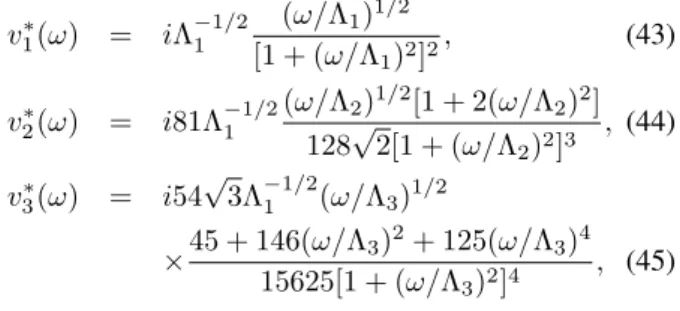
one-photon state respectively. Thus, an initially excited atom makes a transition to the ground state with the emission of a photon. We here choose only three excited levels: the2p state, 3pstate, and4pstate. Then, the form factors corre-sponding to the 2p−1s,3p−1s, and4p−1s transitions become as follows [28, 29],
v∗1(ω) = iΛ
−1/2 1
(ω/Λ1)1/2
[1 + (ω/Λ1)2]2
, (43)
v∗
2(ω) = i81Λ
−1/2 1
(ω/Λ2)1/2[1 + 2(ω/Λ2)2]
128√2[1 + (ω/Λ2)2]3 , (44) v∗
3(ω) = i54 √
3Λ−11/2(ω/Λ3)1/2 ×45 + 146(ω/Λ3)
2+ 125(ω/Λ 3)4
15625[1 + (ω/Λ3)2]4 , (45)
where Λ1 = 8.498 ×10¹⁸ s−1, Λ2 = (8/9)Λ1 s−1, and
Λ3 = (10/12)Λ1 s−1 are the cut-off constants. Note that these form factors have different forms, however they behave in the same way at small energy likeω1/2. The coupling con-stant is also given by λ2 = 6.435×10⁻⁹. The embedded eigenvalues ofH0are defined byωn = 34Ω[1−(n+ 1)−2]
withΩ = 1.55×10¹⁶s−1. To derive these form-factors, we represented|1ωiin the energy-angular momentum basis for
photon [30] as in Ref. [8], incorporating the conservation
of angular momentum and parity in each transition [31]. As was emphasized in Ref. [8], these form-factors are surely an-alytic results without any approximation. The Hamiltonian (1) is then derived within the four-level approximation and the rotating-wave approximation.
In the following, we shall compare the long-time asymptotic-form of A(t) predicted by Eq. (33) and that of Acut(t), which we evaluate numerically. Acut(t)is defined by
Acut(t) =
1 2πi
Z
C
hψ| 1 H−z|ψie
−iztdz.
(46)
The contour C runs clockwise around the half line {re7πi/4|0 ≤ r < ∞} in the complex energy plane. This contour lies on the first Riemann sheet when it goes below the half line, and gets into the second Riemann sheet when it above the half line. Acut(t)is related toA(t)through the equation,
A(t) =Acut(t)− X
zp
Res
µ hψ| 1
H−z|ψie
−izt, z p
¶ , (47)
wherezpis in general the complex pole ofhψ|(H−z)−1|ψi
located in the region between the half lines [0,∞) and {re−πi/4|0 ≤ r < ∞} in the second Riemann sheet. In the weak-coupling case considered here, each ofzpis in the
neighborhood ofωn, and thus the asymptotic form ofAcut(t) and that ofA(t)are expected to exhibit the same behavior at long times, where the power decay dominates over the expo-nential decay [32].
Let us first restrict ourselves to the two initial states: the localized state at the 2plevel |1iand the maximizing state |χi/kχk. Figure 1 shows the time evolution of |Acut(t)|2 and the asymptote of |A(t)|2 for these initial-states. It is clearly seen that|Acut(t)|2’s for these initial states approach to the corresponding asymptotes of |A(t)|2 parallel to t−4, however the difference between them is very small [17]. At t= 105Λ−1
1 , we obtain|Acut(t)/Aasp(t)|2≃0.999for these initial states. Is is worth stressing that this time is very earlier than1/γ1≃1.36×1010Λ−11the lifetime of the2pstate [33], whereγ1= 2πλ2|v1(ω1)|2+O(λ4)≃6.268×10⁸s−1[8].
1 0
5
10
0
10
¡ 1 5
10
¡ 2 0
10
¡ 2 5
jà i=j1i
jà i=jÂi =kÂk
¤ 1
t
j
A
c
u
t
(
t
)
j
2
Figure 1. Square moduli ofAcut(t)’s for initial states|ψi =|1i
and|χi/kχk, and their corresponding asymptotes predicted by Eq. (33) (solid lines). For these initial states,|Acut(t)|
2
shows the same behavior liket−4
We next choose the two special states,|χ⊥
1iand|χ
⊥
2i, as the initial state|ψi. The former is defined by
|χ⊥
1i= f∗
2|1i −f
∗
1|2i p
|f1|2+|f2|2, (48) and the latter is
|χ⊥
2i=
f1f3∗|1i+f2f3∗|2i −(|f1|2+|f2|2)|2i p
|f1f3|2+|f2f3|2+ (|f1|2+|f2|2)2
, (49)
so that they eliminate the factor (31) and satisfy the relations thathχ|χ⊥
1i = 0,hχ|χ
⊥
2i = 0, andhχ
⊥
1|χ
⊥
2i = 0. Figure 2 shows that the time evolution of |Acut(t)|2 for these ini-tial states and for the maximizing iniini-tial state. We clearly find that, as was seen in Fig. 1,|Acut(t)|2for the maximiz-ing initial state (solid curve) asymptotically decays liket−4, whereas |Acut(t)|2 for other initial state (long-dashed and short-dashed curves) follow another decay-law faster than t−4. They seem to be fitted with the power law t−8. For the comparison, we also depict in Fig. 2 the two straight lines
150.0×(Λ1t)−8and30.0×(Λ1t)−8(solid lines), to which |Acut(t)|2for the initial state|χ⊥1iand|χ
⊥
2iapproach respec-tively in this time region.
1 0
5
10
0
¤ 1
t 10
¡ 1 5
10
¡5
j
A
c
u
t
(
t
)
j
2
10
¡ 3 0
4
jà i=jÂi =kÂk
jà i=jÂ
?
1 i
jà i=jÂ
?
2 i
Figure 2. Square moduli of Acut(t)’s for initial states |ψi = |χi/kχk,|χ⊥
1i, and|χ⊥2i. For|χi/kχk,|Acut(t)| 2
shows thet−4
behavior at long times (a solid curve), whereas|Acut(t)|2
for other states exhibit another decay-behavior which is obviously faster than t−4
(long-dashed and short-dashed curves). For the comparison, the two straight lines parallel tot−8
(solid lines) are also depicted.
6
Concluding remarks
We have considered the long-time behavior of the unstable multilevel systems and examined the asymptotic behavior of not only the survivalS(t)but also the totalP(t)probabilities for an arbitrary initial state in the long-time region, where bothS(t)and P(t) obey a power decay law. For the ini-tial state localized at the lowest level, we have found that the SLA results in an underestimation of the asymptotic form of P(t)unlike the result forS(t). We have also discovered two kinds of special initial-state. One of them maximizes the as-ymptotic form ofP(t)at long times, and actually the same state that maximizesS(t). However, for such an initial state,
we only obtain thatP(t)≃S(t)at long times, even though P(t)≥S(t)holds for all timest. The other initial state elim-inates the first term of the asymptotic expansion ofP(t), and also plays the same role forS(t). In addition, we numeri-cally confirm the previous results forS(t)[17] in consider-ation of the spontaneous emission process for the hydrogen atom. Then, we show not only thet−4-decay ofS(t)but also a more faster decay, the latter of which is naively fitted by a power-decay lawt−8. However, we still do not accomplish the derivation of the asymptotic forms for such faster decays. To this end, it will be needed to take into account the zero-energy resonance and the zero-zero-energy eigenstate with an ap-propriate state space [34, 35, 36]. We hope to deal with this issue in the future.
7
Acknowledgments
The author would like to express his gratitude to the organiz-ers of the Second International Workshop DICE2004 Castello di Piombino (Tuscany), September 1-4, 2004,From Decoher-ence and Emergent Classicality to Emergent Quantum Me-chanics. He also would like to thank Professor I. Ohba and Professor H. Nakazato for useful and helpful discussions. This work is partly supported by a Grant for The 21st Cen-tury COE Program at Waseda University from the Ministry of Education, Culture, Sports, Science and Technology, Japan.
References
[1] G. Gamow, Z. Phys.51, 204 (1928).
[2] For a review, see, for example, H. Nakazato, M. Namiki, and S. Pascazio, Int. J. Mod. Phys. B10, 247 (1996).
[3] L. A. Khalfin, Zh. Eksp. Theor. Fiz.33, 1371 (1957) [Sov. Phys. JETP6, 1053 (1958)].
[4] S. R. Wilkinson,et al, Nature (London)387, 575 (1997).
[5] P. T. Greenland, Nature (London)335, 298 (1988).
[6] K. O. Friedrichs, Commun. Pure Appl. Math.1, 361 (1948).
[7] P. Exner,Open Quantum Systems and Feynman Integrals (Rei-del, Doredrecht, 1985).
[8] P. Facchi and S. Pascazio, Phys. Lett. A241, 139 (1998).
[9] I. Antoniou, E. Karpov, G. Pronko, and E. Yarevsky, Phys. Rev. A63, 062110 (2001).
[10] K. Rza¸˙zewski, M. Lewenstein, and J. H. Eberly, J. Phys. B15, L661 (1982).
[11] S. L. Haan and J. Cooper, J. Phys. B17, 3481 (1984).
[12] H. Nakazato, in “Fundamental Aspects of Quantum Physics”, edited by L. Accardi and S. Tasaki (World Scientific, New Jer-sey, 2003).
[13] E. Frishman and M. Shapiro, Phys. Rev. Lett. 87, 253001 (2001); Phys. Rev. A68, 032717 (2003).
[14] I. Antoniou, E. Karpov, G. Pronko, and E. Yarevsky, Int. J. Theor. Phys.42, 2403 (2003).
[16] E. B. Davies, J. Math. Phys.15, 2036 (1974). [17] M. Miyamoto, Phys. Rev. A70, 032108 (2004).
[18] K. Unnikrishnan, Am. J. Phys.65, 526 (1997);66, 632 (1998); F. Lillo and R. N. Mantegna, Phys. Rev. Lett.84, 1061 (2000); 84, 4516 (2000); J. A. Damborenea, I. L. Egusquiza, and J. G. Muga, Am. J. Phys.70, 738 (2002); M. Miyamoto, J. Phys. A35, 7159 (2002); Phys. Rev. A68, 022702 (2003).
[19] M. Miyamoto, Phys. Rev. A69, 042704 (2004).
[20] F. Remacle and R. D. Levine, J. Chem. Phys. 104, 1399 (1996).
[21] E. P. Wigner, Phys. Rev.73, 1002 (1948).
[22] L. P. Horwitz and J.-P. Marchand, Rocky Mountain J. Math. 1, 225 (1971).
[23] A. G. Kofman G. Kurizki and B. Sherman, J Mod Opt.41, 353 (1994).
[24] For the multilevel cases, if all eigenvaluesωnofH0are
posi-tive and non-degenerate, and the coupling constantλis suffi-ciently weak, then we can show that no negative eigenvalues ofHexist.
[25] In fact, by using the technique in the proof of Proposition 3.2.2. in Ref. [7], we can show under our assumption tovn(ω)
that −R0∞dω
′v
n(ω
′)v∗
n′(ω
′)/ω′ = lim
ω↑0snn′(ω) = limω↓0Inn′(ω).
[26] E. T. Copson,Asymptotic Expansions(Cambridge Univ. Press, Cambridge, 1965), Chap. 3.
[27] This interpretation is not necessarily applied to all of the time region. The reason is that such repopulation processes are naively expected to occur under the dominance of the terms ofO(λ2
)for our interaction HamiltonianλV. This does not contradict the behavior ofA(t)(andP(t)) at long times [14].
[28] H. E. Mose, Phys. Rev. A8, 1710 (1973).
[29] J. Seke, Physica A203, 269 (1994).
[30] A. I. Akhiezer and V. B. Berestetskii,Quantum Electrodynam-ics(Interscience, New York, 1965).
[31] Note that the form factors obtained by Ref. [29] are described by the one-photon state with a definite helicity. Thus, to use those results, we need to rewrite such a state in the parity rep-resentation [30]. However, this change makes a difference only in the pre-factor of the results of [29].
[32] The transition time tep from the exponential to the power
decay law is, e.g., approximately 100 lifetimes for the lo-calized state at the2plevel [8, 9]. At this time, we obtain,
|A(tep)|
2
≃4.41×10−55
, an extremely small value [17].
[33] P. Facchi, Ph. D. thesis, Universit`a degli Studi di Bari, 2000.
[34] J. Rauch, Comm. Math. Phys.61, 149 (1978).
[35] A. Jensen and T. Kato, Duke Math. J.46, 583 (1979).