Braz. J. Phys. vol.36 número3A

Determination of Prediction Intervals for a Future Number of Failures: A

Statistical and Monte Carlo Approach

Fortunato S. de Menezes, M´ario J. Ferrua Vivanco,

Departamento de Ciˆencias Exatas, Universidade Federal de Lavras, C.P. 3037, 37200-000, Lavras, MG, Brazil

and Luiz C. Sampaio

Centro Brasileiro de Pesquisas F´ısicas, Rua Dr. Xavier Sigaud, 150, 22290-180, Rio de Janeiro, RJ, Brazil

Received on 7 September, 2005

In this work, we present a new procedure, called sub-sampling, to obtain data concerning time of failure in trials without replacement, (NRT). With this data it is possible to determine the prediction interval (PI) for the future number of failures. We also present analternativeway to evaluate the coverage probability of the prediction interval (PI). The results presented show that the method proposed is reliable and can be useful for the statistical analyses of quality control of processes.

Keywords: Sub-sampling; Weibull Distribution; Prediction Intervals; Coverage Probability; Monte Carlo Simulation

I. INTRODUCTION A. Motivation

The determination of prediction intervals for random quan-tities has been subject of great interest and intensive research for a long time. Its importance is revealed when one addresses the question: If in a system withNcomponents,X quantities failed in the time interval[0,Tc], how many components will

fail in a given future time belonging to the interval[Tc,Tw]? or,

even more, what is the prediction interval(PI)for the number of componentsY that it will fail in the time interval[Tc,Tw]?.

The prediction intervalPI(100(1−α)%)in the time interval

[Tc,Tw]with the confidence level(1−α)is obtained from the

past data of number of componentsXwhich have failed in the time interval[0,Tc]. We illustrate those questions clearly on

Fig. 1.

There are many systems in which the prediction of times of failure of parts is critical, and the implications range from the canonical damage to safety issues. Most of the work which has been developed until now has consideredonlytrials with replacement, namely (RT), where the quantities tested are re-placed in the sample.

Some authors Meeker and Escobar(1998) [5], Ros-tum(1999) [10], Nelson(2000) [7] and Nordman and Meeker(2002) [9] have already discussed this subject. In the last paper, Nordman and Meeker were motivated by the prob-lem of large heat exchangers, that transfer energy to cool down the Nuclear power plants. Due to stress and corrosion the heat exchangers crack over time. Such cracks are detected during planned inspections and the heat exchangers are replaced, or alternatively, isolated from the others. New tubes have to be added then after a given time period, when the number of fail-ures is above a critical value.

It is possible then to measure “ the time until the failure of a component” (e.g., the crack or stress of heat exchangers). The determination of such ”time until the failure of a component” is of great importance to determine prediction intervals (PI).

Usually, the components are replaced in the sample once

they are tested, as long as they have passed in the test. In other words, the components regarded as good according the chosen test are put again the sample. In this way, the good components continues in operation and have a chance to be chosen again in a future time to check its performance and decide whether or not it has failed.

However, there is a class of problems where the replace-ment of good components is not relevant. Suppose we want to acquire a lot ( or sample ) of components, with the previous knowledge that the sample has a certain level of failed com-ponents. Furthermore, we want to acquire the lot as long as the percentage of failure in the sample is less than a given pre-established value. In this work we have developed a method to determine times of failure and, consequently, prediction inter-vals (PI) when the experiments are such that the components used for testing are not replaced in the original sample, even though the result of components tested is negative (e.g., the components tested do not fail). Such method is based upon the measure of “time until the failure of a component” using a new procedure called: sub-sampling.

FIG. 1: Ilustration of the number of components (Y) to fail in the time interval[Tc,Tw]given thatXcomponents failed in the previous time interval[0,Tc]and prediction interval (PI).

replaced in the original sample is a very small fraction of the sample, from where we want to predict something, such that the system as a whole does not change significantly. This is the key point in this procedure and here lies its importance in the prediction intervals (PI).

In the section I.B we present the state of the art concerning the prediction of the future number of failures of components, and the following section I.C shows the purposes to be ful-filled concerning the Non Replacement Trials (NRT) ( or de-structive experiments ). In the section II the Methods are pre-sented, with the sub-sampling strategy (section II.A), the the-ory of prediction intervals (section II.B), the data generation (section II.C) and coverage probability (section II.D). The re-sults and discussion are presented in the section III, along with the probability distribution which best fits the data generated by the sub-sampling procedure (section III.A), the prediction intervals for the problem posed (section III.B) and the alterna-tive coverage probability (ACP) which shows that the method proposed is reliable (section III.C). Finally, the conclusions and the outlook are presented in section IV.

B. State of the art

Results of research about the prediction of random quan-tities have enormous potential for application in engineering and are, indeed, of fundamental importance.

A preliminary study was presented by Nelson(1972) [6]. He established methods to build confidence intervals and hy-pothesis tests for two multinomial proportions. Although the procedures in such work were applied in studies of consumers preferences and election researches, this work was crucial to develop another work published in the year 2000 [7], which has a direct application in engineering.

Meeker and Escobar(1998) [5], developed a method to de-termine the prediction limits (upper and lower) for the future number of fails (Y)in the time interval [Tc,Tw]. Such

pro-cedure is based upon theconditional binomial distributionof Y given that X components have failed in the time interval

[0,Tc].

Rostum(1999) [10], developed statistical models to predict the state of the pipelines in a network of water distribution. Starting from the historical of the past failures in a network of water supply it was possible to predict the future number of failures in each network. These predictions were then used to make decisions about maintenance of the water network. In other words, with his work it may be possible to answer about the following question: Shall we repair points of failure in the network (or sub-network) of water supply, or shall we change anentire pipelinein a given sub-network ?.

Nelson(2000) [7] has established three procedures for the prediction intervals of the number of tubes to fail in compo-nents of heat exchangers, namely (I) the procedure of ratio of probabilities, (II) the procedure of ratio of probabilities sim-plified and (III) the likelihood ratio procedure.

Nordman and Meeker(2002) [9], evaluated the coverage probability for each one of the procedures proposed by Nel-son(2000) [7], concluding that the more appropriate is the

likelihood ratio procedure.

Two aspects must be emphasized in relation to the studies made by Nelson(1972) [6], Nelson(2000) [7] and Nordman and Meeker(2002) [9]:

1. The distribution considered for the variable time until the failure of a component is the Weibull distribution. 2. The tests that evaluatewhether or nota tube is

deterio-rateddoreplace the tube when it is failed.

By contrast, in Agricultural Sciences, particularly in the area of quality control of seeds, we find in the literature some authors Ellis(1984) [1], who suggested the time until a seed has failed follows a Normal distribution. Furthermore, the usual experiments which evaluate whether or not a seed is failed are such that the sub-samples tested are not replaced in the system, Marcos Filho(1987) [4].

Methods to determine the time of failure of a component (and its respective probability distribution) and the prediction interval (PI) of the future number of failures, for experiments in which the components arenotreplaced in the original sam-ple – as the ones done on seeds, were not found in the litera-ture. This research provides a contribution to fill this lack.

C. Purposes

Considering that exist a problematic forNon Replacement Trials (NRT)(e.g., destructive trials), this work has the fol-lowing objectives:

1. Establish a sampling procedure which allows to obtain data for the variable: ”time until the failure of a compo-nent”.

2. Determine the probability distribution for the variable: ”time until the failure of a component”.

3. Determine the prediction interval for the future number of failures.

4. Determine the Coverage Probability (CP) of the predic-tion interval (PI).

II. METHODS

Companies that manufacturefuses(a protection device for safeguarding electric circuits) and the shop dealers, quite of-ten face with the problem for the choice of lots which they intend to acquire. The procedure presented in this section will be related with the problem of the quality control of fuses, where the tests applied to know whether or not a fuse is dete-riorated, are such that the fuses tested are not replaced in the sample which they came from, even though some of the fuses are good (or have passed in the quality test).

Therefore, the goal of this research will be evaluate the vi-ability of acquiring a large lot of fuses, starting from the pre-diction of thenumber of sub-samples of fuses failed in a given time interval(a random quantity). In other words, we start from the test of a small sub-sample of fuses which were taken from a larger sample. With the result which comes up from the test, we can predict what it will be the number of sub-samples of fuses that it will fail in afuturetime interval, thereafter the previous time interval where the test was performed.

The prediction will be made regarding the information ob-tained on the number of sub-samples of fuses which were deteriorated in a time window interval( [0,Tc] )between the

starting of collection of sub-samples tested ( unit of timeT=0 ) until a certain given censured time(T =Tc), which is

pre-established. The study requires the following steps:

(i) the determination of time until a sub-sample of fuses is regarded as deteriorated,

(ii) the determination of a probabilistic distribution of time until the deterioration,

(iii) the determination of the prediction interval ( PI ) for the future number of sub-samples to deteriorate and, (iv) the evaluation of the coverage probability of such prediction interval.

We shall notice thatalthoughthe procedure to be explained will be applied for the case offuses,the method proposed can be applied to any problem in which the sub-samples of components tested are not replaced in the larger sample from where they came from.

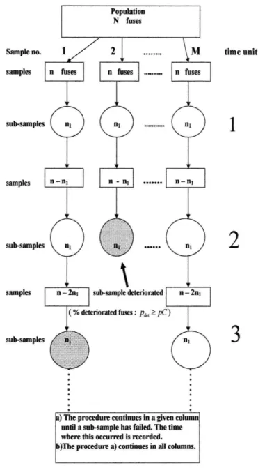
A. Sub-sampling method

As the tests to determine whether or not a fuse is deteri-orated are Non Replacement Trials(NRT), it is not possible to apply directly the methods proposed by the authors men-tioned in the section I B, especially when we wish to know the data related to ”time until the deterioration of a fuse (or sub-sample of fuses)” (and its respective probability distribu-tion). To overcome this problem the following method, called

SUB-SAMPLING, is proposed (see Fig. 2 )

Let us suppose that from a population of N fuses which are packed for sale (illustrated in Fig. 2), we pick upM sam-ples, where each one of them contains n fuses each. From each one of theseM samples, we pickrandomly and system-atically, sub-samples of sizen1. In other words, we now have Msub-samples. In each one of theseMsub-samples we apply the quality test to check the performance of the fuse. Such test is applied in a sub-sample of sizen1( taken from the sam-ple of sizen) to determine the percentage of deteriorated fuses

(pdet). If thepercentage of the deteriorated fuses(pdet)in a

given sub-sample of size (n1) isgreater or equalthan a given valuepC(e.g.,pdet≥pC), which is pre-established, then the

whole sub-sample of sizen is regarded asdeterioratedand we register the time in which the test was performed. From

Fig. 2 we can also see that a sub-sample regarded deterio-rated(e.g., whenpdetin a given sub-sample of sizen1has the value p_det≥pC) implies to stop of picking more sub-samples of sizen1from the respective sample. In other words,the

fail-ure of a given sub-sample of sizen1implies the failure of

the respective sample. A sub-sample regarded not deteri-orated(e.g., when pdet in a given sub-sample of size n1 is

smallerthanpC; pdet<pC) implies in the selection of a new

sub-sample of sizen1, from the sample left. From Fig. 2 it is clear that the sample left now contains n−n1 components, since the firstn1components which were evaluated in the time unit (sayt=1) are set aside oncepdet<pC. Therefore, we

apply the ”fuses quality test” on each new sub-sample of size n1and we check pdet in each new sub-sample of sizen1. In

one hand, for those samples in which the sub-samples presents pdet which DOES overcome the valuepCwe record the time

in which the test was applied and regarded the whole sample as deteriorated for future tests ( for instance, the 2nd sam-ple (column) for the time unitt=2 on Fig. 2). On the other hand, in those samples, in which the pdet DOES NOT

over-come pC, we continue to apply the sub-sampling and there-after the ”fuses quality test”. The procedure continues until the percentage of deterioration in the sub-sample overcomes the valuepC(where the time recorded for the correspondent sample will be the time in which the test was applied and pro-videdpdet≥pC; for instance, the 1st sample (column) at time

unitt =3, see Fig. 2 ) or until we finish with the fuses in a given sample (in such case, the time to be registered will be a censor data).

In this way we can obtain a set ofMdata, correspondent to the set of time units until the deterioration of each one of theM samples (see Fig. 2), from which we will adjust a probability distribution.

B. Prediction Intervals

Once the time until the deterioration of the sub-samples has been obtained as well as its respective probability distribu-tion, the following step will be to determine a prediction in-terval (PI) for the”number of deteriorated sub-samples, in each pack, in a future time interval”. The Fig. 3 illustrates the procedure:

Let us suppose that one package of fuses contains a total of Msamples. It is possible to show that the variablesX,Y and Zfollows a Trinomial Distribution, such thatX+Y+Z=M, with the following probabilities,

• p= probability of occurrence of a failed sub-sample on the time interval[0,Tc].

• q= probability of occurrence of a failed sub-sample on the time interval[Tc,Tw].

• r= probability of occurrence of a failed sub-sample af-terTw.

FIG. 2: Representation of the sub-sampling procedure.

the likelihood ratio procedure in the form described in the fol-lowing:

For the unrestricted model the likelihood function (multinomial) will be,

L(p,q;x,y) = M!

x!y!(M−x−y)! p

x_qy ₍

1−p−q)M−x−y (1)

where the maximum will be given by,

L∗(p,q;x,y) = M! x!y!(M−x−y)!

³x M

´x

׳y

M ´y µ

1−x+y M

¶M−x−y

(2)

The values ofp,qandr, in therestrictedmodel, will de-pend of the data distribution. For instance, the Weibull proba-bility density has the following form,

f(t) = µ_β

η

¶ µ_t

η

¶β−1

FIG. 3: Illustration of the prediction interval ( PI(Y) ) for the time interval[Tc,Tw].

with accumulated distribution function

F(T)≡

Z T

0

f(t)dt =1−exp(−(T/η)β) (4) In other words, if we suppose a Weibull distribution (see Nelson (2000) [7]) with parametersη(scale parameter) and β(shape parameter), for the random variable: time until the deterioration of a sub-sample of fuses, then we have

p≡ Z Tc

0

f(t)dt=1−exp(−(Tc/η)β) (5)

q≡ ZTw

Tc

f(t)dt=exp(−(Tc/η)β)−exp(−(Tw/η)β) (6)

r≡1−p−q=exp(−(Tw/η)β) (7)

Therefore, for aβknown (in whatever way), therestricted

likelihood function to the Weibull distribution will be,

K(η;x,y) =C³1−e(−(Tc/η)β)´x

׳e(−(Tc/η)β)_−e(−(Tw/η)β)´y

׳e(−(Tw/η)β)´M−x−y_{, (8)}

withCgiven by,C= M!

x!y!(M−x−y)!

Since that the value ofY is unknown, in order to maximize K(•)with respect to the scale parameterη, it is needed to run all the values ofY between 0 andM−X. Each value ofY in the interval[0,M−X]will provide a value ofηand, therefore, a maximum value ofK(•), that we will callK∗(•).

It is known that the statistics of likelihood ratio given by,

Q(x,y) =−2 | log(K∗(x,y))−log(L∗(x,y)) | (9) distributes itself as a χ2

(1). Therefore, for any value of the

random variableY, all the values ofQ(X,Y =y)generated, will have identical distributions(χ2

(1gl)). So, it will be possible

to generate a prediction interval(PI)for Y considering the following probability,

P(Q(x,y)≤χ2_(1;α)) =1−α (10) In other words, every value ofY which satisfiesQ(x,y)≤ χ2

(1−α) is contained in the prediction interval with a level of

confidence 100(1−α)%. Consequently, the lowest value of Y(Yin f)and the highest value ofY(Ysup)which satisfy Eq. 10

will be considered the lower and upper limits, respectively, of the prediction interval(PI= [Yin f,Ysup] ).

C. Data generation

The data of the variable time until the deterioration of the sub-samples were generated through Monte Carlo simulation, following the procedure explained in the section II A. For this, it was considered a pack withN=120000 fuses which was di-vided inM=120 samples of sizen=1000. It was considered the values of 1% and 6% for the initial percentages of deteri-oration in each one of theMsamples, since it is supposed that in the beginning of the storage each pack offusescontains a large fraction ofgoodfuses but it may contain a certain frac-tion of failed fuses. The values of 1% and 6% correspond to the fraction of failed fuses in each one of theM=120 ini-tial samples of sizen=1000. Afterwards, it was picked out sub-samples of sizen1=10, in each one of theM samples (see Fig. 2). In the 1st sub-sampling, in each one of theM sub-samples of sizen1 it was made a counting of the num-ber of failed fuses. In the case where the percentage of failed fuses were pdet≥pC, where pC=15% (for 1% and 6% of

initial deterioration of fuses(pini_det)in the sample of sizeM) orpC=50% (for pini_det=6% ), the sub-sample was regarded as failed and it was recorded the value 1 for the respective sample (in other words, the respective sample has failed in the time unitt=1). On the other hand, if the percentage of failed fuses is pdet <pCwe would pass to the 2nd sub-sampling.

Regarding that the percentage of deteriorated fuses increases with time (since we set aside sub-samples of sizen1 which containsgoodfuses and eventually fewfailedfuses) we have to recalculate the percentage of goodfuses, before the 2nd sub-sampling. This new percentage(100p∗%)ofgoodfuses, was obtained subtracting the number of good fuses in 1st sub-sample discarded (of sizen1), from the number of the good fuses existent in the initial sample (of size n) and dividing the result by the number of total fuses in the remained sample (which in the case will be n−n1=990 fuses, see Fig. 2). Fol-lowing this procedure, the percentage ofdeterioratedfuses in the sample left (of sizen−n1) will be(pdet=100(1−p∗)%).

In other words, in the 2nd sub-sampling, the source sample will now haven−n1=990 fuses, with 100p∗% ofgoodfuses and(pdet=100(1−p∗)%)ofdeterioratedfuses. The 2nd

sub-sample of sizen1is taken (see Fig. 2) from the source sample sample (of sizen−n1), and the comparison between pdet (evaluated from this sub-sample size of n1) and pCis

The procedure above was adopted in each sub-sampling un-til a given sub-samplen1has failed. The unit of time in which the sub-sample has failed was regarded as the data for the vari-able ”time until the deterioration of the sample” (the entire column of Fig. 2). At the end of each simulation we end up with a set of 120 data, one for each one of theM=120 sam-ples (or columns of Fig. 2). With this set of 120 data, we have adjusted the probability distribution.

D. Coverage probability

Considering that, givenX=x, the conditional distribution of the random variable Y is binomial with the parameters

³

M−X,π=_q+q_r´,M defined in the section II A and withq andrdefined in Eqs. (5)- (7); we have the value ofπgiven by,

π=1−exp[(Tc/η)β−(Tw/η)β] (11)

In the work of Nordman and Meeker(2002) [9] it was pre-sented a suggestion given by Wayne Nelson in which the cov-erage probability (CP) for the prediction interval (PI) with a nominal level of confidence of 100(1−α)% may be deter-mined by the average of the probabilitiesP(Yin f≤Y≤Ysup|X)

found for each value ofX. In other words,

CP(PI(100(1−α)%)) =Ex[P(Yin f ≤Y ≤Ysup)] (12)

The expression showed on Eq. 12 is true and determine the coverage probability. However, its value is computationally difficulty to obtain for two reasons:

a) The procedure of maximization of Eq. 8 generates a maximum likelihood estimation for the parameterηfor each value ofY. Therefore, as π depends on η (see Eq. 11), we would have a value ofπfor each possible value ofY.

b) The discrete values ofY that are found inside the pre-diction intervalPI(Y) = [Yin f,Ysup], determined

accord-ing to Eq. 10, are not necessarily contiguous. In other words, the prediction intervalPI(Y) = [Yin f,Ysup]may

be composed by sub-intervals not contiguous.

An alternative analysis to evaluate the coverage probabil-ity is presented in this work. Such analysis is based upon the counting of values ofY(obtained through simulation, accord-ing the procedure presented in Section II A and II C) which are inside thetheoreticalprediction intervalPI(Y) = [Yin f,Ysup]

(which was obtained according the procedure showed in the Section II B).

The percentage of values ofY which are inside the predic-tion intervalPI(Y) = [Yin f,Ysup]will be regarded as the

alter-native coverage probability (ACP).

The results of such analysis are presented in Section III C.

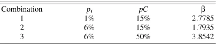
TABLE I: Values ofβ(shape parameter of Weibull distribution) ob-tained from simulations with the number of samplesM=20000. pi denotesinitialpercentage of deterioration in one sample;pCdenotes themaximumallowed deterioration in one sub-sample of sizen1;

andβ, the shape parameter of Weibull distribution. In all calcula-tionsn1=10.

Combination pi pC β

1 1% 15% 2.7785

2 6% 15% 1.7935

3 6% 50% 3.8542

III. RESULTS AND DISCUSSION A. Probability distribution

According the procedures detailed in the Sections II A and II C it was performed 6000 simulations for each pair of combination(pi,pC)(where, pi, is the initial percentage of

deterioration and ,pC, the maximum acceptable percentage of deterioration in each sub-sample of sizen1) (See Table I). Those simulations generate, each one,M =120 data corre-spondent to the variable: ”time until the failure of the sub-sample”( or sample, as it was emphasize in the Section II A ). With those data it was established a probabilistic distribution which offers the best fitting.

From Eq. 4, and using the survival function(S(T) ) esti-mated according to Kaplan and Meier (1958) [11],

S(T)≡1−F(T) =exp(−(T/η)β) (13) we can easily see that,

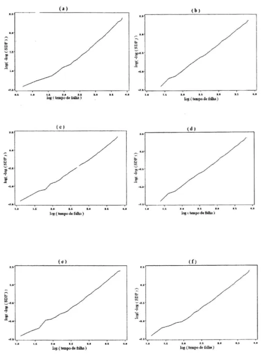
log(−log(S(T))) =βlog(T

η) (14) Fig. 4 presents the illustration of 6 graphs which represents 6 data sets selected randomly among all the simulations per-formed. These graphs clearly show that the data sets can be adjusted by the Weibull distribution, what allows us to use the methodology to estimate the prediction intervals presented in the Section II B.

The linear tendency of the graphs observed in Fig. 4 demon-strates that the Weibull distribution adjusts very well to the variable ”time until the failure of the sub-samples of fuses” in non replacement trials.

Considering now that the distribution which suits best to the simulations performed is the Weibull distribution, it was estimated (through simulation results) the shape parameter(β)

more suitable for each combination of(pi,pC).

FIG. 4: Plots of the Weibull probabilities for the set of data of time until the failure of samples of fuses, for 6 simulations selected among the 6000 simulations. Thehorizontal axisrepresentslog(Tf)and thevertical axisrepresentslog(−log(S(Tf))), whereS(Tf) =1−F(Tf)is the survival function estimated according the Kaplan-Meier (1958) method [11], for the time until the failure,Tf.

in Table 1. Such values will be used to determine the predic-tion intervals.

The values ofβ(the shape parameter of the Weibull distri-bution) used for each combination of(pi,pC)are presented in

Table I. Those values ofβare used to determine the predic-tion intervals (PI) for the number of samplesM=120. The reason for using the values ofβobtained forM=20000 and

nottheβvalues obtained for the number of samplesM=120, is that we are looking for a stable value ofβ. This argument is

inspired onPhysical argumentsofComputational Physics

FIG. 5: Plot of the shape parameter(β), as function of the number of samplesM.

choice made.

Another alternative to obtain approximate values of β is through the determination of the confidence intervals optimal conditioned, discussed by Mahdi (2003) [3].

B. Prediction Intervals

It was determined the prediction intervals for the random variableY: Future number of failures of samples in the time interval[Tc,Tw] = [10,20]units of time, for each combination

(pi,pC), following the procedure detailed in the Section II B.

The nominal level of confidence 1−α used was 0.95 and the number of samples wasM=120.

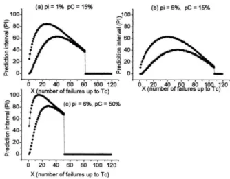
On Fig. 6 it is presented the prediction intervals (PI), ob-tained as a function of the number of sub-samples failed (X) in the time interval [0,Tc) = [0,10), for each set of values

presented on Table I, namely (pi=1%,pC=15%), (pi=

6%,pC=15%)and(pi=6%,pC=50%).

We shall notice that in all 3 cases presented on Fig. 6, we observe that as the number of fails X in the time interval

[0,Tc) = [0,10)increases, thewidthof the prediction

inter-valdecreases. Such behavior is reasonable if we bear in mind that as we havemoreinformation (the number of components failed,X) in the initial time interval ([0,Tc)), the determination

of the prediction interval (PI), which depends on this previous information, will be more precise, and therefore its width de-creases. Following this reasoning we shall believe that for values ofX very close to zero provides prediction intervals (PI) quite wide as shown on Fig. 6. Nevertheless, we shall notice that the level ( 1−α) for all the intervals is the same. We believe that the points of discontinuity observed on Fig. 6 ((a) atX=80, (b) atX=108 and (c) atX=45) should nei-ther be interpreted as prediction intervals of zero width, nor as a pointed prediction ofY. As in the discontinuity points the

FIG. 6: Prediction interval forY: future number samples failed in the time interval[Tc,Tw] = [10,20]units of time, for a nominal level of probability of 0.95.

prediction intervals do not offer any width, there would not be any sense to evaluate the prediction intervals for those points.

C. Alternative Coverage probability

As it was mentioned in Section II D, we will present an

alternative methodto evaluate the coverage probability (CP), hereafter calledACP. Here we propose a simpler method, as we judge, to confirm this. This method require 4 stages:

1. The generation, through Monte Carlo simulation, of 6000 data sets, according the procedure explained in Section II A. Each data set contains M =120 data of time of failure for the M=120 samples used (see Fig. 2).

2. The recording, for each simulation in step (1), ofX: the number of samples failed in the time interval[0,Tc) =

[0,10). As we have usedM=120 samples, obviously X≤M.

3. Afterwards, according the theoretical procedure showed on Section II B, the determination of the pre-diction interval for Y: the future number of failures in the time interval[Tc,Tw] = [10,20]for each possible

value ofX ≤M, regardless this value has (or has not) appeared in the simulation results (step 2).

4. The recording, for each simulation in step (1), the num-ber of failuresY⋆ which have occurred in the time win-dow interval[Tc,Tw] = [10,20]. The Y⋆ is obtained in

the following way. Let beX1 the number of failures in the time interval[0,Tc) = [0,10), and let beY1 the

num-ber of failures in the time interval[0,Tw] = [0,20]. Y⋆is

5. The determination of the percentage (or fraction) of values recorded in step (4) ( The Y⋆ values obtained through simulation results), which are inside the respec-tive theoretical prediction interval (PI) obtained in step (3).

We can notice from Fig. 7, that in the 6000 simulations per-formed for each combination (pi,pC), we did not find

neces-sarily all the possible values ofXwith the value of ACP near the nominal level (95%) or alternatively, 0.95. The reason for that is that Monte Carlo simulations for each pair(pi,pC)

provide an interval of values ofX that is finite and dependent upon the values(pi,pC). This means that in the region where

theACPis null wedo nothave data set and therefore we can-not calculateproperlytheACP. On the other hand, for each value ofXfound in the Monte Carlo simulation, the number of failures occurred in the time interval[Tc,Tw] = [10,20], is

in-side the respective theoretical prediction interval (PI) obtained in the step 3 of this procedure and illustrated on Fig. 6. This result is a good indicator of the reliability of the method.

FIG. 7: Alternative Coverage probability(ACP)for the prediction intervalPI(Y): number of failures in the time interval[10,20]units of time for each combination of values(pi,pC)showed on Table 1.

What Fig. 7 also shows is that for fixedpC(the maximum allowed percentage of deterioration in each sub-sample of size n1=10), the number of failuresX increases for increasing values ofpi(the initial percentage of deterioration in the

sam-ple sizen=1000).

IV. CONCLUSIONS

In this work we have proposed a method called SUB-SAMPLING, to obtain data of the time of failure in trials without replacement, ( NRT ), through Monte Carlo simu-lation. The data set obtained through this method has been showed to be well adjusted by the Weibull distribution for the data of time of failure. It was possible to obtain the prediction interval for afuturenumber of failures with the knowledge

onlyof the number of failures in thepasttime.

The results obtained with the alternative procedure to eval-uate the coverage probability (ACP), indicate that the method, suggested in this work, to determine the prediction intervals in non replacement trials is reliable.

As a forthcoming work is the determination of the pair of probabilities(pi,pC)from the histogram of frequencies ofX

(i.e.,the number of failed components up toTC) by the

simula-tion data for a number of samplesM. Then, through a single real experiment in a single sample, we determine the num-ber of failured components untilTC (e.g., the value of XEX P

); with this date, and in association with the most probable value of the number of failed components for the sameTC

(X_SIM∗ ) from the simulation data for M samples ( which is dependent on the simulated pair of probabilities(pi,pC)), we

obtain through the matching ofXEX PwithXSIM∗ the

correspon-dent pair of probabilities(pi,pC). This is a key point, as we

can determine from a single real experiment the value ofXEX P

for a givenTC and, with the complementary simulation data

through the most probable value ofX_SIM∗ from the histogram of frequency ofX forMsamples, the degree of deterioration pi (for a given cut-off probability pC) for the single sample

where the real experiment was made.

Acknowledgements

We wish to thank Willian Q. Meeker and Daniel J. Nord-man for clarifying us on the subtle points regarding the Cover-age Probability and the reliability of the method in their paper Nordman and Meeker (2002) [9].

[1] R.H. Ellis, The meaning of viability,Hortsience,26,9 (1984). [2] D.P. Landau and K. Binder,A Guide to Monte Carlo Simulation

in Statistical PhysicsCambridge: Cambridge University Press (2000).

[3] S. Mahdi, Optimal conditional interval for the shape paramenter of a Weibull distribution,Brazilian Journal of Probability and Statistics,17, 57-74 (2003).

Departamento de Agricultura e Horticultura, ESALQ/USP (1987).

[5] W. Meeker and L. Escobar,Statistical Methods for Reliability Data, John Wiley: New York (1998).

[6] W. Nelson, Statistical methods for the ratio of two multinomial proportions,The American Statisticiam,26, 22-27 (1972). [7] W. Nelson, Weibull prediction of a future number of

fail-ures, Quality Reliability Engennering International,16, 23-26 (2000).

[8] M. Newman and G. Bakerma,Monte Carlo Methods in Statis-tical Physics, Oxford: Orford University Press (1999).

[9] D.J. Nordman and W.Q. Meeker, Weibull prediction for a future number of failures,Technometrics,44, no.1, 15-23 (2002). [10] J. Rostum Decision Support Tools for Sustainable Water

Net-work Management, A research project supported by the Eu-ropean Commission under the fifth framework program, bf http://www.unife.it/care-w (1999).