Artigo
A MODEL OF FUZZY TOPOLOGICAL RELATIONS FOR SIMPLE
SPATIAL OBJECTS IN GIS
Um modelo de relações topológicas fuzzy para objetos espaciais em GIS
BO LIU1,2,3
DAJUN LI2
JIAN RUAN2
LIBO ZHANG4
LAN YOU5,1*
HUAYI WU1
1 State Key Laboratory of Information Engineering in Surveying, Mapping and Remote Sensing, Wuhan
University, 129 Luoyu Road, Wuhan 430079, China
2 Faculty of Geomatics, East China Institute of Technology, 418#Guanglan Road, Nanchang 330013, PR,
China
3 Key laboratory of watershed ecology and geographical environment monitoring, National
Administration of Surveying, Mapping and Geoinformation, 418#Guanglan Road, Nanchang 330013, PR, China
4 National Quality Inspection and Testing Center for Surveying and Mapping Products, 28Lianhuachi West
Road, Hai dian District, Beijing 100830, PR, China
5 Faculty of Computer Science and Information Engineering, Hubei University,
368Youyi Avenue, Wuhan 430062, PR, China
[email protected]; [email protected]; [email protected]; [email protected]; [email protected];[email protected]
Abstract:
Bol. Ciênc. Geod., sec. Artigos, Curitiba, v. 21, no 2, p.389-408, abr-jun, 2015. models.
Keyword:Topological Relation; Simple Spatial Objects; Fuzzy Topology; Model; GIS. Resumo:
O objetivo deste artigo é apresentar um novo modelo de relações topológicas fuzzy para objetos espaciais simples em Sistemas de Informações Geográficas (SIG). Aplica-se o conceito de espaço topológico fuzzy a objetos fuzzy simples para resolver as relações topológicas de modo mais eficiente e acurado. Inicialmente é proposta uma nova definição para segmentos de linha fuzzy e para regiões fuzzy com base na topologia computacional. Em seguida propõe-se um novo modelo para calcular as relações topológicas fuzzy entre os objetos espaciais. A análise do
novo modelo aponta: (1) relações topológicas de dois objetos “crisp”; (2) relações topológicas entre um objeto “crisp” e um objeto fuzzy; (3) relações topológicas entre dois objetos “crisp”.
Finalmente, discutem-se alguns exemplos para demonstrar a validade do modelo, por meio de um experimento e comparações entre modelos existentes. É possível demonstrar que o método proposto pode realizar distinções mais precisas e á mais expressivo do que os modelos fuzzy existentes.
Palavras-chave:Relações Topológicas; Objetos Espaciais Simples; Topologia Fuzzy; Modelo; GIS.
1. Introduction
Geographical information sciences (GIS) commonly deal with geographical phenomena modeled by crisp points, lines, and regions, features which are clearly defined or have crisp boundaries. However, geospatial data are always uncertain or fuzzy due to inaccurate data acquisition, incomplete representation, dynamic change, and the inherent fuzziness of geographical phenomena itself. In GIS, many studies have been devoted to modeling topological relations, specifically the modeling of fuzzy topological relations between simple spatial objects. Topology is a fundamental challenge when modeling the spatial relations in geospatial data that includes a mix of crisp, fuzzy and complex objects. Two mechanisms, the formalization and reasoning of topological relations, have become popular in recent years to gain knowledge about the relations between these objects at the conceptual and geometrical levels. These mechanisms have been widely used in spatial data query (Egenhofer, 1997, Clementini et al., 1994), spatial data mining (Clementini et al., 2000), evaluation of equivalence and similarity in a spatial scene (Paiva, 1998), and for consistency assessment of the topological relations of multi-resolution spatial databases (Egenhofer et al., 1994, 1995; Du et al., 2008a, b). Diloet al. (2007) defined several types and operators for modeling spatial data systems to handle fuzzy information. Shi et al. (2010) and Liu et al. (2011) developed a new object extraction and classification method based on fuzzy topology.
relations between two regions and can be considered as an extension of the crisp case. They can be implemented on spatial databases at less cost than other uncertainty models and are useful when managing, storing, querying, and analyzing uncertain data. For example, Egenhofer and Franzosa (1991a, 1994, 1995) and Winter (2000) modeled the topological relations between two spatial regions in two dimensional space (2-D) based on the 4-intersection model and ordinary point set theory. Li et al. (1999), Long and Li (2013) produced a Voronoi-based 9-intersection model based on Voronoi diagrams. Cohn et al. (1996, 1997) discovered forty-six topological relations between two regions with indeterminate boundaries based on Region Connection Calculus (RCC) theory (Randell et al., 1992). Clementini and Di Felice (1996a, b, 1997) used extended 9-intersection model to classify forty-four topological relations between simple regions with broad boundaries. The extended 9-intersection model substantially agrees with the RCC model, though the former removes two relations considered as invalid in the geographical environment. The extended 9-intersection model can be extended to represent topological relations between objects with different dimensions, like regions and lines, while the RCC model can only be applied to relations between regions. Tang and Kainz (2002), Tang et al. (2005), Tang (2004) applied fuzzy theory and a 9-intersection matrix and discovered forty-four topological relations between two simple fuzzy regions. Shi and Liu (2004) discussed fuzzy topological relations between fuzzy spatial objects based on the theory of fuzzy topology. Du et al. (2005a, b) proposed computational methods for fuzzy topological relations description, as well as a new fuzzy 9-intersection model. Liu and Shi (2006, 2009), Shi and Liu(2007) defined a computational fuzzy topology to compute the interior, boundary, and exterior parts of spatial objects, and based on the definition, Liu and Shi(2009) proposed a computational 9-intersection model to compute the topological relations between simple fuzzy region, line segment and fuzzy points, but the model did not give the topological relations between two simple fuzzy regions, and did not compute the topological relations between one simple fuzzy spatial object and one simple crisp spatial object.
To further investigate the application of fuzzy topological relations in GIS, on the basis of previous researches, this study develops a new model of describing the fuzzy topological relations for simple fuzzy objects. The new model not only computes the topological relations between simple crisp spatial objects, but also computes the topological relations between simple fuzzy spatial objects.
The remainder of this paper is organized as follows. In section 2, some basic concepts of fuzzy topology, computational fuzzy topology and the definitions of simple fuzzy spatial objects in GIS are detailed; In the Section 3, the new definition of simple fuzzy spatial objects is presented, and a new model of fuzzy topological relations for simple fuzzy spatial objects is proposed; In Section 4, some examples are discussed to validate the proposed method. Finally, some conclusions are drawn in Section 5.
2.
A Brief Summary of Computational Fuzzy Topology
Bol. Ciênc. Geod., sec. Artigos, Curitiba, v. 21, no 2, p.389-408, abr-jun, 2015.
topology is the fundamental theory for modeling topological relations between simple crisp spatial objects in GIS. By extension, fuzzy topology is a generalization of ordinary topology that introduces the concept of membership value and can be adopted for modeling topological relations between spatial objects with uncertainties. Zadeh (1965) introduced the concept of fuzzy sets, and fuzzy set theory. Fuzzy topology was further developed based on the fuzzy sets (Chang, 1968; Wong, 1974; Wu and Zheng, 1991; Liu and Luo, 1997).Liu and Shi (2006, 2009), and Shi and Liu (2007) defined a computational fuzzy topology to compute the interior, boundary and exterior of spatial objects. The computation is based on two operators, the interior operator and the closure operator. Each interior operator corresponds to one fuzzy topology and that each closure operator also corresponds to one fuzzy topology (Liu and Luo, 1997). The research detailed in this paper extends this work by defining fuzzy spatial objects. However, it is important to review basic concepts in fuzzy set theory as well as simple fuzzy objects in GIS.
2.1 Basic Concepts
We focus on the two-dimensional Euclidean plane R2, with the usual distance and topology.
Fuzzy topology is an extension of ordinary topology that fuses two structures, the order and topological structures. Fuzzy interiors, boundaries, and exteriors play an important role in the uncertain relations between GIS objects. In this section we first present the basic definitions for fuzzy sets, and then the definitions for fuzzy mapping.
Definition 2.1 (Fuzzy subset). Let X be a non-empty ordinary set and I be the closed interval [0,
1].
An I-fuzzy subset on X is a mappingA:X I, i.e., the family of all the [0,1]-fuzzy or I-fuzzy
subsets on X is just IX; consisting of all the mappings from X to I. Here, IX is called an I-fuzzy
space. X is called the carrier domain of each I-fuzzy subset in it, and I is called the value domain
of each I-fuzzy subset on X. AIXis called a crisp subset on X, if the image of the mapping is
the subset of
0,1 I .Definition 2.2 (Rules of set relations). Let A and B be fuzzy sets in X with membership
functions A(x) andB(x), respectively. Then, 1) A=B, iff A(x)=B(x) for all x in X;
2) AB, iff A(x)B(x) for all x in X;
3) C=AB, iff C(x)=max [A(x),B(x)] for all x in X;
4) D=AB, iff D(x)=min [A(x),B(x)] for all x in X;
5) E=X\A, iff E(x)=1-A(x) for all x in X.
X
I
. is called an I-fuzzy topology on X, and (IX, ) is called an I-fuzzy topological space
(I-fts), if satisfies the following conditions:
1) 0,1 ,2) If A, B , then AB , then 3) Let
Ai:iJ
,where J is an index set,and iJ Ai.
Where, 0 means the empty set and 1 means the whole set X. The elements in are called
open elements and the elements in the complement of are called closed elements, and the set of the complement of an open set is denoted by.
Definition 2.4 (Interior and closure). For any fuzzy setAIX , the interior of A is defined as
the join of all the open subsets contained in A, denoted by o
A . The closure of A is defined as the
meeting of all the closed subsets containing A; denoted byA.
Definition 2.5 (Fuzzy complement). For any fuzzy set A, we defined the complements of AbyAC(x)1A(x); denoted by AC.
Definition 2.6 (Fuzzy boundary). The boundary of a fuzzy set A is defined as: AAAC.
Definition 2.7 (Closure operator). An operator X X
I I
:
is a fuzzy closure operator if the following conditions are satisfied:
1)(0)0; 2)(A)A, for allAIX ; 3)(AB)(A)(B); 4)((A))(A), for all X
I A .
Definition 2.8 (Interior operator). An operator :IX IXis a fuzzy interior operator if the following conditions are satisfied:
1)(1)1; 2)A(A), for allAIX ; 3)(AB)(A)(B); 4)((A))(A), for all X
I A .
Definition 2.9 (Interior and closure operators). For any fixed[0,1], both operators, interior
and closure, are defined as
0 ( )
) ( )
( ) (
x A if
x A if x A x
A and
1 ) ( )
(
1 ) ( 1
) (
1
x A if x
A
x A if x
A respectively, and
can induce an I-fuzzy topology (X,,1)in X, where
A :AIX
are the open sets and
X
I A
A
1 :
1
are the closed sets. The elements in and 1 satisfy the
relations( )C ( C)1 A
A , for all fuzzy sets A, i.e., the complement of the elements in the
Bol. Ciênc. Geod., sec. Artigos, Curitiba, v. 21, no 2, p.389-408, abr-jun, 2015. given in Liu and Shi (2006).
To study topological relations, it is essential to first understand the properties of fuzzy mapping, especially homeomorphic mapping since topological relations are invariant in homeomorphic mappings. The following section presents a number of definitions related to fuzzy mapping. Let X Y
I
I , be I-fuzzy spaces, f :X Y an ordinary mapping. Based on f :X Y , define
I-fuzzy mapping f:IX IYand its I-fuzzy reverse mapping f:IX IYby
Y X
I I
f: ,
otherwise y f x if x A V y A f
, 0
) ( ,
) ( )
)( (
1
,AIX,yY
X Y
I I
f: ,f(B)(x)B(f(x)),BIY,xX
WhileI [0,1].
Let( X,)
I , (IY,)be I-fts’s, f:(IX,)(IY,)is called I-fuzzy homeomorphism, if it is
bijective, continuous, and open (Liu and Luo, 1997). One important theorem to check an I-fuzzy
homeomorphism is that, as proved by Shi and Liu (2007). Let X Y
I B I
A , ,
let( X,)
I ,(IY,)be I-fts’s induced by an interior operator and closure operators. Then
) , ( ) , (
: X Y
I I
f is an I-fuzzy homeomorphism if and only if f :X Y is a bijective mapping. Meanwhile, for the topology induced by these two operators, when checking a homeomorphic map, we only have to check whether there is a one-to-one correspondence between the domain and range.
2.2 Fuzzy Simple Spatial Objects in GIS
Based on the definitions presented in section 2.1, Liu and Shi developed fuzzy definitions for the basic elements in GIS (Liu and Shi, 2006, 2009; Shi and Liu, 2007), summarized here as follows:
Definition 2.10 (fuzzy point, Figure 1(a)). An I-fuzzy point on X is an I-fuzzy subsetXIX,
defined as:
otherwise x y if y
x
0 )
(
.
Definition 2.11 (Simple fuzzy line, Figure 1(b)). A fuzzy subset in X is called a simple fuzzy
line (L) if L is a supported connected line in the background topology (i.e., a crisp line in the
background topology).
Definition 2.12 (Simple fuzzy line segment, Figure 1(b)). The simple fuzzy line segment (L) is
segment (i.e., a crisp line segment in the background topology) in the background topology and 2) (( ) 1
L L
L C ) has at most two supported connected components.
Definition 2.13 (Simple fuzzy region, Figure 1(c)). A simple fuzzy region is a fuzzy region in
X where: 1) for any(0,1), the fuzzy setAandA(A)C A1are two supported connected
regular bounded open sets in the background topological space. And, 2) in the background topological space, any outward normal from Supp (A) must meet Supp (A) and have only one
component.
Interior
Boundary
Interior Boundary
(a)Fuzzy point (b) Fuzzy line segment (c) Fuzzy region
Figure1: (a) Fuzzy point for a given ; (b) Fuzzy line segment for a given ; (c) Fuzzy region
for a given (Liu and Shi 2009)
On the basis of definitions for simple fuzzy points, line segments and regions, Shi and Liu (2007) provide an example of computing the interior, boundary, and exterior of spatial objects for differentvalues, and the interior, boundary, and exterior of spatial objects were confirmed for each givenvalue. Based on the fuzzy definitions, Liu and Shi (2009) proposed a new3 3
integration model to compute the topological relations between simple fuzzy region, line segment and fuzzy points. The element ( fXABdV) of the new3 3 integration model is the ratio of the area( or volume) of the meet of two fuzzy spatial objects in a join of two simple
spatial object(here a join of two fuzzy objects means “union” of two fuzzy objects; a meet of two fuzzy objects means “intersection” of two fuzzy objects(Liu and Shi, 2009)). And it was difficult
to change or transform the new3 3 integration model to describe the topological relations between one simple crisp spatial object and one simple fuzzy spatial object.
Based on existing related studies, in the next section, we will discuss the method of fuzzy topological relations for simple spatial objects.
3. Modeling Fuzzy Topological Relations for Simple Spatial Objects
in GIS
3.1 A New Definition for Simple Fuzzy Spatial Objects
Bol. Ciênc. Geod., sec. Artigos, Curitiba, v. 21, no 2, p.389-408, abr-jun, 2015. 1968), the fuzzy point definition remains the same as Definition 2.10.
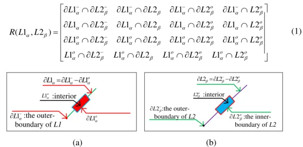
Definition 2.14 (inner and outer boundary of simple fuzzy line segment, Figure 2(a)), for
given , the interior and boundary of simple line segment L(as shown in figure1(b)) are
confirmed, separately, can be regarded as a simple crisp line segment. Therefore, we defineLas the outer-boundary of L, andLoas the inner-boundary of L,Loas the interior of L,
andLas the boundary of L(as shown in figure4(a)):L L Lo. So, a simple fuzzy line
segment L for given can be written as: L L L Lo Lo .
Definition 2.15 (inner and outer boundary of simple fuzzy region, Figure 2(b)), for a
given, the interior and boundary of fuzzy region A (as shown in figure1(c)) is confirmed,
separately, can be regarded as a simple crisp region. Therefore, we defined A as the
outer-boundary of A, andAoas the inner-boundary of A, Aoas the interior of A andAas the
boundary of A (as shown in figure4 (b)): A AAo. So the fuzzy region A for givencan
be expressed as: o o
A A A A
A . Meanwhile, AandAocan be considered as two
simple crisp regions.
:the inner-boundary of L :the
outer-boundary of L
L o
L
o
L L
L
:interior
o
L
:the outer-boundary of A
:the inner-boundary of A
o
A
A
o
A A A
:interior
o A
(a) Fuzzy line segment L (b) Fuzzy region A
Figure 2: (a) The inner-outer boundary of simple fuzzy line segment L for given ; (b) The
inner-outer boundary of simple fuzzy region A for given
Based on the above definitions, (1) to a simple fuzzy line segment L for given, ifL Lo,
that isL 0, andLL L Lo, it means L is a simple crisp line segment; (2) to a fuzzy
region A for given, ifA Ao, that isA 0,AA AAo, it means A is a simple
crisp region.
3.2 A New Model of the Fuzzy Topological Relations for Simple Spatial
Objects
In this paper, we just discussed the topological relations between two simple fuzzy line segments, the topological relations one simple fuzzy line segment and one simple fuzzy region, and the topological relations between two simple fuzzy regions, as follows.
(I) Topological relations between two simple fuzzy line segments
For one simple fuzzy line segment L1 for given (figure3 (a)), and the other simple fuzzy line
segment L2 for given (figure3 (b)). The topological relations between L1 and L2 can be
computed by4 4 intersection model as equation (1).
o o o o o o o o o o o o o o o o L L L L L L L L L L L L L L L L L L L L L L L L L L L L L L L L L L R 2 1 2 1 2 1 2 1 2 1 2 1 2 1 2 1 2 1 2 1 2 1 2 1 2 1 2 1 2 1 2 1 ) 2 , 1
( (1)
:the outer-boundary of L1
L1 o
L1
o
L L L111
:interior o
L1
:the inner-boundary of L2 :the
outer-boundary of L2
L2
o
L2
o
L L L2 22
:interior
o
L2
(a) (b)
Figure 3: (a) A simple fuzzy line segment L1 for given; (b) A simple fuzzy line segmentL2
for given
There are three different topological relations between L1 and L2, as follows:
1) if o
L L1 1
,that is 1 0
L , L1L1 L1 L1o ; if o
L L2 2
,that
isL2 0, o
L L L
L2 2 2 2. Thus, L1 and L2 are crisp line segments, the equation (1)
can be turned into 4-Intersection Model (4IM) (Egenhofer and Franzosa, 1991a) or 9-Intersection Model (9IM) (Egenhofer and Franzosa, 1991b), the topological relations between L1 and L2 are
computed by 4IM or 9IM. 2) If o
L L1 1
, that isL1 0, L1L1 L1L1o, L1 is a simple crisp line segment.
If o
L L2 2
, that is 2 0
L , o o
L L L
L L
L2 2 2 2 2 2, L2 is a simple fuzzy
line segment, and comprised of four components 2
L , L2 , L o
2
and L o
Bol. Ciênc. Geod., sec. Artigos, Curitiba, v. 21, no 2, p.389-408, abr-jun, 2015.
while o
L L
L2 2 2
. The equation (1) can be turned into24intersection model as
equation (2). o o o o o o o o L L L L L L L L L L L L L L L L L L R 2 1 2 1 2 1 2 1 2 1 2 1 2 1 2 1 ) 2 , 1
( (2)
3) If o
L L1 1
, that is 1 0
L ,L1L1 L1L1 L1o L1o,L1 is a simple fuzzy
line segment, and comprised of four components L1 , L1 , L1o and L1 , in o
addition, o
L L
L1 1 1
. If o
L L2 2
, that is 2 0 L , o o L L L L L
L2 2 2 2 2 2, L2 is a simple fuzzy line segment too, comprised of
four components 2
L ,L2 ,L2o and L2 , in addition,o o
L L
L2 2 2
. Thus, the
topological relations between L1 and L2 can be computed by44intersection model as equation
(1).
(II)Topological relations between one simple fuzzy line segment and one simple fuzzy region
For one simple fuzzy line segment L1 for a given (figure4 (a)), there is one simple fuzzy
region A1 for given (figure4 (b)).The topological relations between L1 and A1 can be
computed by4 4 intersection model as equation (3).
o o o o o o o o o o o o o o o o A L A L A L A L A L A L A L A L A L A L A L A L A L A L A L A L A L R , )
( (3)
:the
inner-boundary of L
:the
outer-boundary of L
L o
L
o
L L
L
:interior o L :the outer-boundary of A
o
A
:the inner-boundary of A
A
o
A A A
:interior
o
A
(a) (b)
Figure 4: (a) A simple fuzzy line segment L for given ; (b)A simple fuzzy region A for
given
There are four different topological relations between L1 and A1, as follows:
1) If o
L L
, that isL 0,LL L Lo , L is a simple crisp line segment. If o
A A
that isA 0, o
A A A
A , and A is a simple crisp region. The equation (3) can be
turned into 4-Intersection Model (4IM) (Egenhofer and Franzosa, 1991a) or 9-Intersection Model (9IM) (Egenhofer and Franzosa, 1991b), the topological relations between L and A are
computed by 4IM or 9IM. 2) If o
L L
, that isL 0,LL L Lo , L is a simple crisp line segment. If o
A A
,
that isA 0, o o
A A A A A
A , A is a simple fuzzy region, comprised of
four components
A ,A,AoandAo, in addition, o
A A A
. The equation (3) can be
turned into24intersection model as equation (4).
o o o o o o o o A L A L A L A L A L A L A L A L A L R , )
( (4)
3) If L Lo
, that is 0
L ,LL L L Lo Lo, L is a simple fuzzy line segment,
comprised of four componentsL ,L,LoandLo , in addition, L L Lo .If o
A A
,
that isA 0, o
A A A
A , A is a simple crisp region. The equation (3) can be turned
into24intersection model too, as equation (5).
o o o o o o o o L A L A L A L A L A L A L A L A A L R , )
( (5)
4) If L Lo
, that is 0
L , LL LL Lo Lo , L is a simple fuzzy line
segment, comprised of four components L , L , Lo and Lo , in addition,
o
L L L
.If o
A A
, that is 0
A , o o
A A A A A
A , A is a simple
fuzzy region, comprised of four components
A ,A,AoandAo, in addition, o
A A A
.
The topological relations between L and A can be computed by44intersection model as equation (3).
(III) Topological relations between two simple fuzzy regions
For one simple fuzzy region A1 for given (figure5 (a)), the other simple fuzzy region A2 for
given (figure5 (b)). The topological relations betweenA1 and A2 can be computed
Bol. Ciênc. Geod., sec. Artigos, Curitiba, v. 21, no 2, p.389-408, abr-jun, 2015. o o o o o o o o o o o o o o o o A A A A A A A A A A A A A A A A A A A A A A A A A A A A A A A A A A R 2 1 2 1 2 1 2 1 2 1 2 1 2 1 2 1 2 1 2 1 2 1 2 1 2 1 2 1 2 1 2 1 ) 2 , 1
( (6)
o
A1
:the inner-boundary of A1
A1
o
A A A111
:interior
o A1
:the outer-boundary of A2
o
A2
:the inner-boundary of A2
A2
o
A A A2 2 2
:interior
o
A2
(a) (b)
Figure 5: (a) A simple fuzzy region A1 for given; (b) A simple fuzzy region A2 for given
There are three different topological relations between A1 and A2, as follows:
1) if o
A A1 1
, that is 1 0
A , A1A1 A1A1o , A1 is a simple crisp region.
If o
A A2 2
, that is 2 0
A , o
A A
A
A2 2 2 2, A2 is a simple crisp region too.
Therefore, the equation (6) can be turned into 4-Intersection Model (4IM) (Egenhofer and Franzosa, 1991a) or 9-Intersection Model (9IM) (Egenhofer and Franzosa, 1991b), the topological relations between A1 and A2 are computed by 4IM or 9IM.
2) If o
A A1 1
, that isA1 0, A1A1 A1A1o, A1 is a simple crisp region. If
o
A A2 2
, that is 2 0
A , o o
A A
A A
A
A2 2 2 2 2 2, A2 is a simple fuzzy
region, comprised of four components 2
A , A2 , A o
2
and A o
2 , in
addition, o
A A
A2 2 2
.The equation (6) can be turned into24intersection model as
equation(7). o o o o o o o o A A A A A A A A A A A A A A A A A A R 2 1 2 1 2 1 2 1 2 1 2 1 2 1 2 1 ) 2 , 1
( (7)
3) If A A o
1
1
, that is 1 0
A , andA1A1 A1 A1A1o A1o, A1 is a simple
fuzzy region, comprised of four components A1 , A1 , A1o and A1 , in addition, o
o
A A
A1 1 1
. If o
A A2 2
, that is 2 0
A , o o
A A
A A
A
A2 2 2 2 2 2,
A2 is a simple fuzzy region, comprised of four componentsA2,A2,A2oandA2 , in o
addition, o
A A
A2 2 2
.The topological relations between
by4 4 intersection model as equation (6).
Through the above description, the equation(1), (3) and (6)are equivalent, only replacing the elements of the44intersection model, the 4IM or 9IM, equation(2), (4) ,(5), (7) are only the new44intersection models’(equation(1), (3), (6)) exception, and all the equation can describe the topological relations respectively.
In this section, we develop a new44intersection model to compute the fuzzy topological relations between simple spatial objects. An analysis of the new model exposes: (1) the topological relations between two simple crisp line segments; (2) the topological relations between two simple fuzzy line segments; (3) the topological relations between one simple crisp line segment and one simple fuzzy line segment; (4) the topological relations between one simple crisp line segment and one simple crisp region; (5) the topological relations between one simple crisp line segment and one simple fuzzy region; (6) the topological relations between one simple fuzzy line segment and one simple crisp region; (7) the topological relations between one simple fuzzy line segment and one simple fuzzy region; (8) the topological relations between one simple crisp region and one simple fuzzy region; (9) the topological relations between two simple crisp regions; (10) the topological relations between two simple fuzzy regions.
In the next section, we will focus on taking some examples to demonstrate the validity of the new model by comparing with existing models.
4. Experiment and Comparison
The new4 4 intersection model can identify the topological relations between two simple spatial objects. The following content will take some examples to demonstrate the validity of the new model, and compare with the existing fuzzy models.
4.1 Experiment Results
In this section, we will take some examples to demonstrate the validity of the new model. 1) A simple crisp line segment L1 (figure6 (a)), a simple fuzzy line segment L2 for given=0.4
(figure6 (b)).The topological relation between them was shown in figure 6(c). Since the intersection of two sets can be either 0 or 1, the topological relation between L1 and L2 can be
computed by equation (2) as:
1 1 0 0
0 0 0 0 ) 2 , 1 (L L
Bol. Ciênc. Geod., sec. Artigos, Curitiba, v. 21, no 2, p.389-408, abr-jun, 2015.
:the inner-boundary of L2
:the outer-boundary of L2
L2
o
L2
o L L L222
:interior
o
L2
:the outer-boundary of L1
L1
:interior
o
L1
(a) (b) (c)
Figure 6: (a) Simple crisp line segment L1; (b) Simple fuzzy line segment L2 for given=0.4;
(c) The topological relation between L1 and L2
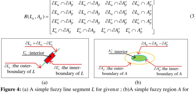
2) A simple fuzzy line segment L1 for given =0.5(figure7 (a)), a simple fuzzy line segment L2
for given =0.3 (figure7 (b)).The topological relation between them was shown in figure7(c).Since the intersection of two sets can be either 0 or 1, the topological relation between
L1 and L2 can be computed by equation (1) as:
0 0 1 0
0 0 1 0
1 1 1 0
1 0 1 0 )
2 , 1 (L L
R .
:the inner-boundary of L1
:the outer-boundary of L1
L1 Lo
1
o L L L111
:the inner-boundary of L2
:the outer-boundary of L2
L2
o L2
o L L L222
:interior :interior
o L1
o L2
(a) (b) (c)
Figure 7: (a) Simple fuzzy line segment L1 for given =0.5; (b) Simple fuzzy line segment L2
for given=0.3; (c) The topological relation between L1 and L2
3) A simple fuzzy line segment L1 for given =0.5 (figure8 (a)), a simple fuzzy region A1 for
given=0.4 (figure8 (b)). The topological relation between them was shown in figure8(c). Since the intersection of two sets can be either 0 or 1, the topological relation between L1 and A1 can
be computed by equation (3) as:
0 0 1 1
0 0 1 1
1 1 1 0
:the outer-boundary of A1 :the
inner-boundary of L1 :the
outer-boundary of L1
L1 o
L1
o
L L L111
:interior
o L1
o
A1
:the inner-boundary of A1
A1
o
A A A111
:interior o
A1
(a) (b) (c)
Figure 8: (a) Simple fuzzy line segment L1 for given =0.5; (b) Simple fuzzy region A1 for
given=0.4; (c) The topological relation between L1 and A1
4) A simple crisp line segment L1 (figure9 (a)), a simple fuzzy region A1 for given=0.4 (figure
9(b)). The topological relation between them was shown in figure9(c). Since the intersection of two sets can be either 0 or 1, the topological relation between L1 and A1 can be computed by
equation (4) as:
1 1 1 1
1 0 0 0 ) 1 , 1 (L A R
o
A1
:the inner-boundary of A1
A1
o
A A A111
:interior o
A1
:the outer-boundary of L1
L1
:interior
o L1
:the outer-boundary of A1
(a) (b) (c)
Figure 9: (a) Simple crisp line segment L1; (b) Simple fuzzy regionA1 for given=0.4; (c) The
topological relation between L1 and A1
5) A simple fuzzy line segment L1 for given =0.5 (figure10 (a)), a simple crisp region A1
(figure10 (b)). The topological relation between them was shown in figure10(c). Since the intersection of two sets can be either 0 or 1, the topological relation between L1 and A1 can be
computed by equation (5) as:
1 1 1 1
1 1 0 0 ) 1 , 1 (L A
R .
:the inner-boundary of L1 :the
outer-boundary of L1
L1 o
L1
o
L L L111
:interior
o
L1
1 A
:interior o
A1
:the outer-boundary of A1
(a) (b) (c)
Figure 10: (a) Simple fuzzy line segment L1 for given=0.5; (b) Simple crisp region A1; (c)
The topological relation between L1 and A1
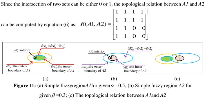
6) A simple fuzzy regionA1 for given =0.5 (figure11 (a)), a simple fuzzy region A2 for
Bol. Ciênc. Geod., sec. Artigos, Curitiba, v. 21, no 2, p.389-408, abr-jun, 2015.
Since the intersection of two sets can be either 0 or 1, the topological relation between A1 and A2
can be computed by equation (6) as:
0 0 1 1
0 0 1 1
1 1 1 1
1 1 1 1 ) 2 , 1 (A A
R .
o
A1
:the inner-boundary of A1
A1
o A A A111
:the outer-boundary of A2
o A2
:the inner-boundary of A2
A2
o A A A2 2 2
:the outer-boundary of A1
:interior :interior
o
A1 o
A2
(a) (b) (c)
Figure 11: (a) Simple fuzzyregionA1for given=0.5; (b) Simple fuzzy region A2 for
given=0.3; (c) The topological relation between A1and A2
7) A simple fuzzy region A1 for given =0.5 (figure12 (a)), a simple crisp region A2 (figure12
(b)), the topological relation between them was shown in figure12(c). Since the intersection of two sets can be either 0 or 1, the topological relation between A1 and A2 can be computed by
equation (7) as:
1 1 1 1
1 1 1 1 ) 2 , 1 (A A
R .
o
A1
:the inner-boundary of A1
A1
o
A A A111
:the outer-boundary of A2
2
A
:interior :interior
o
A1 o
A2
(a) (b) (c)
Figure 12: (a) Simple fuzzyregionA1 for given=0.5; (b) Simple crisp region A2; (c) the
topological relation between A1 and A2
4.2 Comparison with Existing Models
In dealing with fuzzy spatial objects, Cohn and Gotts (1996) proposed the ‘egg-yolk’ model with
model
B A B A B A B A B A B A B A B A B A B AR9 , , which was proposed by Egenhofer and Franzosa
(1991b), Clementini and Di Felice defined a region with a broad boundary, by using two simple regions (Clementini and Di Felice, 1996, 1997). This broad boundary is denoted byA. More precisely, a broad boundary is a simple connected subset of R2 with a hole. Based on empty and
non-empty invariance, Clementini and Di Felice’s Algebraic
model,
B A B A B A B A B A B A B A B A B A B A
R9 , , gave a total of 44 relations between two spatial
regions with a broad boundary.
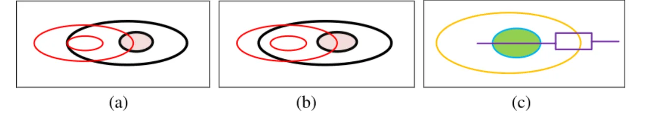
For example, as shown in figure13(a, b), the extended 9-Intersection model proposed by
Clementini and Di Felice (1996,1997) yielded the same matrix,
1 1 0 1 1 1 1 1 0 ) , ( 9 A B
R , that is to
say, the topological relations are same, but they are obviously different from each other as shown in figure13(a, b) . Meanwhile, Liu and Shi (2009) proposed a 33 integration model to compute the topological relations between fuzzy line segments, and discovered sixteen topological relations between simple fuzzy region and simple fuzzy line segment. However, the33integration model could not get the topological relation as shown in figure 13(c). Then, we will discuss the topological relation as shown in figure 13 of using the new44intersection model (equation (1), (6)) in this paper.
We use the new44intersection model to obtain the44matrix, as follows:
For figure13 (a), the topological relation matrix is:
0 0 1 0 0 0 1 1 1 1 1 1 1 1 1 1 ) 2 , 1 (A A
R ;
For figure13 (b), the topological relation matrix is:
0 0 1 0 0 0 1 0 1 1 1 1 1 1 1 1 ) 2 , 1 (A A
R ;
For figure13 (c), the topological relation matrix is:
0 0 1 1 0 0 1 1 1 1 1 0 0 0 1 0 ) 1 , 1 (L A
Bol. Ciênc. Geod., sec. Artigos, Curitiba, v. 21, no 2, p.389-408, abr-jun, 2015.
(a) (b) (c)
Figure 13: (a), (b) Two different topological relations between region A1 and A2; (c) Topological
relation between a simple fuzzy line segment L1 and a simple fuzzy region A1
Through the above comparison analysis, the new proposed model (when taking different values ofand) not only can compute the topological relations as listed in existing studies (Liu and Shi, 2009; Cohn et al. , 1996, 1997;Clementini and Di Felice,1996,1997), but also the topological relations not currently listed.
5. Conclusion and Discussion
Fuzzy topological relations between simple spatial objects can be used for fuzzy spatial queries and spatial analyses. This paper presented a model of fuzzy topological relations for simple spatial objects in GIS. Based on the research of Liu and Shi, we propose a new definition for simple fuzzy line segments and simple fuzzy regions based on the computational fuzzy topology. We also propose a new44intersection models to compute the fuzzy topological relations between simple spatial objects, as follows: (1) the topological relations of two simple crisp objects; (2) the topological relations between one simple crisp object and one simple fuzzy object; (3) the topological relations between two simple fuzzy objects. We have discussed some examples to demonstrate the validity of the new model. Through an experiment and comparisons of results, we showed that the proposed method can make finer distinctions, as it is more expressive than the existing fuzzy models.
In this study, fuzzy topology is dependent on the values of andused in leveling cuts, and different values of and generate different fuzzy topologies and may have different topological structures. When some applications of fuzzy spatial analyses, an optimal value ofandcan be obtained by investigating these fuzzy topologies (Liu and Shi, 2006, Shi and Liu, 2007).
ACKNOWLEDGEMENTS
The authors would like to thank the Editor and the two anonymous reviewers whose insightful suggestions have significantly improved this letter.
REFERENCES
Chang, C.L. “Fuzzy topological spaces.” Journal of Mathematical Analysis and Applications,
(24), 182-190, 1968.
Clementini, E., Di Felice, D.P. “An algebraic model for spatial objects with indeterminate boundaries.” In: Burrough, P.A., Frank, A.U. (Eds.), Geographic Objects with Indeterminate Boundaries. Taylor & Francis, London and Bristol, 155-169, 1996a.
Clementini, E., Sharma, J., Egenhofer, M.J. “Modeling topological spatial relations: Strategies for query processing.”Computers and Graphics, 18(6), 815-822, 1994.
Clementini, E., Di Felice, P. “A model for representing topological relationships between complex geometric features in spatial databases.” Information Sciences, 90(1), 121-136,
1996b.
Clementini, E., Di Felice, P. “Approximate topological relations.” International Journal of Approximate Reasoning, 16(2), 173-204, 1997.
Clementini, E., Di Felice, P., Koperski, K. “Mining multiplelevel spatial association rules for objects with a broad boundary.”Data & Knowledge Engineering, 34(3), 251-270, 2000. Cohn, A.G., Gotts, N.M. “The ‘egg-yolk’ representation of regions with indeterminate
boundaries.” In: Burrough, P.A., Frank, A.U. (Eds.), Geographic Objects with Indeterminate Boundaries, Taylor & Francis, London and Bristol, 171-187, 1996.
Cohn, A.G., Bennett, B., Gooday, J., Gotts, N.M. “Qualitative spatial representation and reasoning with the region connection calculus.”GeoInformatica, 1(1), 1-44, 1997.
Dilo, A., de By, R.A., Stein, A. “A system of types and operators for handling vague spatial
objects.”International Journal of Geographical Information Systems, 21(4), 397-426, 2007. Du, S.H., Qin, Q.M., Wang, Q., Ma, H. “Evaluating structural and topological consistency of
complex regions with broad boundaries in multi-resolution spatial databases.” Information Sciences, 178(1), 52-68, 2008a.
Du, S.H., Guo,L., Wang, Q., Qin, Q.M. “Efficiently computing and deriving topological relation matrices between complex regions with broad boundaries.” ISPRS Journal of Photogrammetry & Remote Sensing, (63), 593-609, 2008b.
Du, S.H., Qin, Q.M., Wang, Q. “Fuzzy description of topological relations I: a unified fuzzy
9-intersection model.” In: Wang, L., Chen, K., Ong, Y.S. (Eds.), Advances in Natural Computation, Lecture Notes in Computer Science, 3612, 1260-1273, 2005a.
Du, S.H., Qin, Q.M., Wang, Q. “Fuzzy description of topological relations II: computation methods and examples.” In: Wang, L., Chen, K., Ong, Y.S. (Eds.), Advances in Natural Computation, Lecture Notes in Computer Science, 3612, 1274-1279, 2005b.
Egenhofer, M., Franzosa, R. “Point-set topological spatial relations.” International Journal of Geographical Information Systems, 5(2), 161-174, 1991a.
Egenhofer M, Herring J. “Categorizing Binary Topological Relationships between Regions,
Lines, Points in Geographic Databases.” Oronoi: Technical Report, Department of
Surveying Engineering, University of Maine, Oronoi, ME, 1991b.
Egenhofer, M., Franzosa, R. “On the equivalence of topological relations.”International Journal of Geographical Information Systems, 8(6), 133-152, 1994.
Egenhofer, M., Mark, D. “Modeling Conceptual Neighborhoods of Topological Line-Region
Bol. Ciênc. Geod., sec. Artigos, Curitiba, v. 21, no 2, p.389-408, abr-jun, 2015.
Egenhofer, M.J. “Query processing in spatial-query-by-sketch.” Journal of Visual Languages and Computing, 8(4), 403-424, 1997.
Li, C.M., Chen, J., Li, Z.L. “Raster-based method or the generation of Voronoi diagrams for
spatial entities.” International Journal of Geographical Information Systems, 13(3), 209,
1999.
Long Z.G, Li S.Q. “A complete classification of spatial relations using the Voronoi-based nine-intersection model.” International Journal of Geographical Information Science,
27(10), 2006-2025, 2013.
Liu, K.F., Shi, W.Z. “Computation of fuzzy topological relations of spatial objects based on
induced fuzzy topology.” International Journal of Geographical Information Systems, 20(8),
857-883, 2006.
Liu, K.F., Shi, W.Z. “Quantitative fuzzy topological relations of spatial objects by induced fuzzy
topology.” International Journal of Applied Earth Observation and Geoinformation, (11),
38-45, 2009.
Liu, K.F., Shi, W.Z., Zhang H. “A fuzzy topology-based maximum likelihood classification.” ISPRS Journal of Photogrammetry and Remote Sensing, (66), 103-114, 2011.
Liu, Y.M., Luo, M.K. “Fuzzy Topology.”Singapore: World Scientific, 1997.
Paiva, J.A.C. “Topological equivalence and similarity in multi-representation geographic
databases.”Ph.D. Dissertation. Department of Surveying Engineering, University of Maine,
1998.
Randell D.A., Cui Z., Cohn A.G. “A spatial logic based on regions and connection.” In Proceedings 3rd International Conference on Knowledge Representation and Reasoning,
25–29 October 1992, San Mate, M. Kaufmann, California, 165-176, 1992.
Shi, W.Z., Liu, K.F. “Modelling fuzzy topological relations between uncertain objects in GIS. “Photogrammetric Engineering and Remote Sensing, 70(8), 921-930, 2004.
Shi, W.Z., Liu, K.F. “A fuzzy topology for computing the interior, boundary, and exterior of
spatial objects quantitatively in GIS.”Computer and Geoscience, 33(7), 898-915, 2007. Shi, W.Z., Liu, K.F., Huang C.Q. “A Fuzzy-Topology-Based Area Object Extraction Method.”
IEEE Transactions on Geoscience and Remote Sensing, 48(1), 147-154, 2010.
Tang, X.M., Kainz, W. “Analysis of topological relations between fuzzy regions in general fuzzy topological space.” In: Proceedings of Spatial Data Handling Conference, Ottawa, Canada,
2002.
Tang, X.M., Kainz, W., Yu F. “Reasoning about changes of land covers with fuzzy settings.” International Journal of Remote Sensing, 26(14), 3025-3046, 2005.
Tang, X.M. “Spatial object modeling in fuzzy topological spaces: with applications to land cover change.”Ph.D. Dissertation. University of Twente, 2004.
Winter, S. “Uncertain topological relations between imprecise regions.” International Journal of Geographical Information Science, 14(5), 411-430, 2000.
Wong, C.K. “Fuzzy points and local properties of fuzzy topology.” Journal of Mathematical Analysis and Applications, (46), 316-328, 1974.
Wu, G., Zheng, C. “Fuzzy boundary and characteristic properties of order homomorphisms.” Fuzzy Sets and Systems, (39), 329-337, 1991.