Empirical analysis of Brazilian banks’ capital buffers during the period
2001-2011*
Vinícius Cintra Belém Banco do Brasil, Brasília, DF, Brazil
Ivan Ricardo Gartner
Universidade de Brasília, Programa de Pós-Graduação em Administração, Brasília, DF, Brazil
Received on 12.16.2013 – Desk acceptance on 01.27.2014 – 4th version accepted on 12.29.2015.
ABSTRACT
International literature indicates that the capital buffers held by banks result notably from the trade-off that exists between the cost of hol-ding capital, adjustment costs, and bankruptcy costs, which all have a direct impact on banks’ capital structures. The aim of this paper is to study the degree of sensitivity of Brazilian banks’ capital buffers to the determining factors established in the literature, by using a sample of 121 banks, covering the period from 2001 to 2011. The empirical analysis that was carried out found that there was a significant cost of adjusting capital buffers for the Brazilian banks. At the same time, bankruptcy cost indicated a positive relationship between risk profile and capital buffers, while the cost of holding capital did not exhibit statistical significance in the analysis.
Keywords: banking institutions, banking risk, regulatory capital buffers, dynamic panel data.
1 INTRODUCTION
will not be remunerated, thus penalizing the opportuni-ty cost of shareholders’ financial resources. Therefore, the higher the cost to banks of holding this capital, the smaller the capital buffer to be held should be.
To these two costs can be added bankruptcy cost, which refers to the cost that an extrapolation of the mi-nimum capital ratio can result in from regulators, or to the cost of not returning credit loaned by banks to their clients.
As well as these three main factors, various others discussed in the literature can affect a bank’s decisions to hold capital above the regulatory minimum required, such as the size of the bank, the country’s economic cycles, the demand for credit, merger and acquisitions operations, and banking regulation, among others. Thus, banks, at the time they outline their capital struc-ture policies, aim to maximize the return on existing ca-pital, considering the trade-off between the three main types of costs mentioned previously and other factors that can affect their capital structures.
Fonseca and González (2010) analyzed whether the-se three costs, as well as other variables, determined banks’ capital buffers in around 70 countries, including 56 Brazilian banks, between 1995 and 2001. After this period, there have been few studies focused on the Bra-zilian case, which motivated the development of this paper. Thus, this study aims to contribute to the state of current knowledge regarding the factors that have in-fluenced Brazilian banks’ decisions when defining their capital structures, and, consequently, in determining capital buffer amounts, given that this is a relevant issue due to it involving an economic sector that is more and more competitive in a more intense regulatory environ-ment. The study analyzed the behavior of 121 Brazilian banks between 2001 and 2011, a period in which there was great change in the architecture of the international financial system, above all after the crisis triggered in July 2007 in the United States.
The article is organized in the following way: the first section presents the motivation and reason for the study; the second presents a brief breakdown of banking regulations and the state of current knowledge from the literature on capital buffers. In section 3, the methodo-logical procedures for the study are described, notably the variables used, and specification of the econometric model. In section 4, an empirical analysis is carried out, and section 5 presents the article’s conclusions.
Banking institutions play a fundamental part in how economic systems operate, especially due to their role as financial intermediaries. In this role, banking insti-tutions capture the resources of agents with surpluses (investors) in order to subsequently transfer them to agents with deficits (assignees of credit). In exercising this role of intermediation between investors and re-ceivers of credit, banks are exposed to various types of risks, which can weaken their financial situation. In or-der to avoid one bank’s financial problems compromi-sing the whole system of financial intermediation in a market, regulatory bodies require banks to hold capital reserves in order to face the risks inherent to their bu-siness, aiming to maintain a safe environment for the financial system.
Studies carried out in the international field, among which those of Jokipli and Milne (2008, 2011), and Stolz and Wedow (2011) stand out, have found empirical evi-dence that most banks have held levels of capital in re-serves above the minimum amount required by regula-tory bodies. This difference between the capital reserve held by banks and the level of regulatory capital, which is called the regulatory capital buffer, constitutes the fo-cus of this study. It aims, specifically, to analyze whether the factors proposed by the literature as determinants for holding regulatory capital buffers are also relevant in the area of Brazilian banking institutions.
According to Alencar (2011), capital buffer theory, which favors holding capital above the minimum level required by regulators, has gained popularity among theories which study capital requirements and the ad-justment of banks’ portfolios.
Estrella (2004) and Ayuso, Perez, and Saurina (2004) propose that the amounts of capital buffers to be held by banks are given by the trade-off between three main factors: the cost of adjusting capital; the cost of holding capital; and the cost of bankruptcy.
The cost of adjusting capital derives from the costs generated by raising new funds to recompose capital le-vels. For Rime (2001), if banks fall below the regulatory minimum, they can suffer penalties imposed by regula-tory agencies, or they might even have to cease opera-tions. Gropp and Heider (2010) state that, as a result of this risk and the high cost of raising capital in the short run, banks opt for holding capital buffers.
The cost of holding capital affects decisions regar-ding the amount to be held by banks, since such capital
2 BANKING REGULATION AND REGULATORY CAPITAL
In 1988, the Bank of International Settlements (BIS) met to create an agreement (Basel I) that set the mini-mum amount of capital that banks should hold, aiming to stabilize the international financial system.
were exposed to (Pillar II).
In order to verify banks’ solvency levels, regulatory bodies use the Basel ratio, which is an indicator that ve-rifies whether banks capital (Reference Equity) is suffi-cient to cope with the risks that are inherent to their operations, which are shown in the form of Required Reference Equity (RRE). This verification is related to the context of Pillar I of Basel II, which determines ins-titutions’ minimum capital requirements. The Basel ra-tio defined by the Basel Committee is 8% and that adop-ted by the Brazilian Central Bank (BACEN) since 1997 has been 11%.
For regulatory purposes, during the period covered by the study, bank capital was divided into two levels. Level I capital is where banks’ base capital lies. For Glantz (2007, p. 338), level I capital is the most valuable to banks. The main components that can be classified into this level are ordinary shares, perpetual preferred shares, characterized as non cumulative, and retained earnings, where the majority of reserves and the pre-miums paid in the acquisition of investments should be excluded.
As well as level I capital, regulators also consider other instruments as being capital for coping with the risks banks face, known as level II capital. Some sha-reholder equity accounts that have not composed level I capital are included in this capital, as well as debt ins-truments that do not form part of shareholder equity, such as hybrid capital and debt instruments, and subor-dinated debt instruments.
According to Vallascas and Hagendorff (2013), the regulatory capital required by banks serves to increase certainty and solidity, holding sufficient capital to cope with the risks that their assets might be exposed to.
2.1 Capital Buffers
For Peura and Keppo (2006), the capital structure chosen by banks is, in essence, defined by their risk ma-nagement decisions, since banks do not use capital as a form of financing, but rather, as a buffer against their assets exposed to risk, which need to be managed in or-der to satisfy a minimum capital required with relation to possible future adversities. According to the authors, it is implicit that violation of this minimum capital value results in costs for banks, or a need for restrictions on their portfolios of assets, or new capitalization. Elizalde and Repullo (2007) also add support to this idea, clai-ming that the non observation of a regulatory minimum could even result in banks closing, prompting capital levels to be held that are above the minimum required.
Shrieves and Dahl (1992) relate some factors that affect the capital held by banks, such as bankruptcy costs, caused by the exposure of their assets to risk, and management aversion to risk, originating from sha-reholder pressure over managers to hold lower leverage. The authors also mention the need to observe the mini-mum capital level required by regulators and regulatory costs as factors that affect capital held.
As well as the risks and costs that banks can incur in not managing to hold the minimum capital required, they also need to uphold a capital structure compatible with market expectations and which allows them to ex-ploit future investment opportunities, having sufficient capital available to grant new loans and carry out the in-vestments demanded by the market (Berger, Herring, & Szegö, 1995; Jokipii & Milne, 2008). Moreover, Estrella (2004) highlights that banks’ capital structures should take optimization of their capital into account, conside-ring all costs and expected returns.
Estrella (2004) and Ayuso et al. (2004) stress that banks’ decision models with regards to their capital is the result of the trade-off of three different types of costs – the cost of holding capital, the cost of bankruptcy, and the cost of adjustment – and, as they are obliged to hold the minimum capital determined by regulators, their decisions can only occur in relation to the size of the buffer to be held.
For Ayuso et al. (2004), holding capital has a direct cost for banks, because, given information asymmetry, this source of funds is more expensive than other finan-cing options. In the pecking order theory described by Myers (1984), retention of earnings by companies is the first option for financing, since funds generated inter-nally do not have transaction costs.
Given these factors, retention of earnings is one of the ways that banks use most to increase their capital buffers, implying that returns have a positive impact on them. On the other hand, Stolz and Wedow (2011) claim that high returns can also be interpreted as the abili-ty of a bank to maintain this level of profitabiliabili-ty, me-aning these returns are subsequently incorporated into the bank’s capital, sustaining the growth of their assets weighted by risk. Thus, a negative impact of returns on capital buffers can also be expected.
In relation to bankruptcy cost, holding a capital bu-ffer reduces the likelihood of bank failure, loss of repu-tation, and the costs of resulting legal action (Ayuso et al., 2004). In the concept of bankruptcy cost, the cost of failure is also considered, which contemplates the li-kelihood of losses resulting from the investments made by banks. For Bikker and Metzmakers (2004), this cost depends specifically on the risk profile of each bank.
The concept of bankruptcy cost also considers risks of non compliance with the regulatory minimum requi-red and the costs resulting from this, such as restrictions that can be imposed by regulators (Ayuso et al., 2004).
The risks a bank is exposed to can be measured in different ways, but, according to Jokipii & Milne (2011), this measurement is not simple and each proxy used exhibits a limitation. Basically, an ex ante measurement of risks can be considered, anticipating their effects, or an ex post one, observing the effects after their occur-rence.
bank’s capital and the risk from its portfolio of invest-ments is expected, given that banks with greater risk should hold more capital. For Ayuso et al. (2004), and Boucinha and Ribeiro (2007), ex post measurement of risk exhibits a negative relationship between a bank’s ca-pital and the risk from its portfolio of investments. This negative relationship can be explained by the consump-tion of capital that will occur when risk materializes, in the form of losses or through provisions that affect bank capital. For Jokipii and Milne (2008), risk measured ex post should also exhibit a positive relationship between a bank’s capital and the risk from its portfolio of invest-ments, since ex post risk also demonstrates the risk pro-file of banks.
In relation to adjustment cost, Ayuso et al. (2004) ar-gue that changes in bank capital levels incur costs, and the main cost of adjustment is related to the problem of information asymmetry. As banks have a greater level of information than the market, they require higher re-muneration to make recomposing their capital possible. Stolz and Wedow (2011) also argue that banks cannot make instantaneous adjustments in their capital or in their risk (portfolio of investments). As capital rearran-gements or sales of or changes in investments require some time to be carried out, banks need to hold capital buffers. Thus, adjustment cost should exhibit a positive relationship with bank capital.
Jokipii and Milne (2008) argue that, among the fac-tors that affect capital buffers, the one that stands out most is bank size. Stolz and Wedow (2011) show some cases in which the size of banks can affect capital buffers. Larger banks can have greater investment and diversifi-cation opportunities, thus presenting a lower likelihood of suffering a negative shock in their capital, with them being able to hold smaller buffers as insurance for this risk. For Tabak, Li, Vasconcelos, and Cajueiro (2013),
the use of this variable in studies regarding financial institutions is important given economies of scale, and can explain the individual characteristics of each bank.
Another reason is that in the case of financial crises, there is a greater likelihood that large banks would be rescued by governments, avoiding a potential systemic effect. This rescue of large banks by governments is cal-led “too big to fail” (Berger et al., 1995; Rime, 2001; Ayu-so et al., 2004; Lindquist, 2004; Jokipii & Milne, 2008; Araújo, Jorge & Linhares, 2008).
A great amount of the literature regarding capital buffers addresses the influence of the economic cycle on the behavior of banks’ capital buffers (Ayuso et al., 2004; Lindquist, 2004; Ferreira, Noronha, Tabak & Ca-juerio, 2010; Stolz & Wedow, 2011). Such studies have aimed to observe whether the behavior of capital bu-ffers was pro-cyclical or counter-cyclical. If the beha-vior was pro-cyclical, it is expected that during econo-mic growth there would be an increase in the volume of loans, without sufficient funds being raised to counter the risks on them, causing reductions in capital buffers. If the behavior was counter-cyclical, it is expected that, during economic growth, there would be an increase in the volume of loans, with more, or at least enough, fun-ds being raised to counter the risks on the loans, causing an increase or maintenance of capital buffers.
In a way, one of the reasons for seeking the rela-tionship between the economic cycle and capital buffers lies in that fact that, with growth in the economy, banks grant more credit, possibly affecting their capital bu-ffers. Thus, another variable that can have an influence over banks’ capital buffers is borrowers’ demand for cre-dit. When this demand for credit increases, and banks supply it through loans, assets exposed to risk increase, thus resulting in the consumption of banks’ capital bu-ffers.
3 STUDY METHODOLOGY
3.1 Population and Sample
he period covered in this study was from the 1st quarter of 2001 to the 4th quarter of 2011, amounting to 44 quarters in total. Some ilters were used in order to improve the qua-lity of the data, such as using banks that presented a greater historic series than 15 months and excluding those that alrea-dy sufered intervention or liquidation by BACEN, those that were under investigation for indications of fraud in their i-nancial statements, and those that exhibited volatility in their capital bufer volatility coeicients greater or equal to 2. hus, the sample used in this study comprised 121 banks.
he data employed for calculating the dependent varia-ble and the majority of explanatory variavaria-bles was obtained
from the “50 Biggest Banks and the Brazilian Financial Sys-tem Consolidated Report” (2012), available from the BACEN
website. he explanatory variable Variation in GDP, used as a proxy for the economic cycle, was obtained from the Bra-zilian Institute of Geography and Statistics (IBGE) website. he dummy variable Mergers and Acquisitions was obtained from the Mergers and Acquisitions report from the company RISKbank, which carried out a survey of these operations over the period from 1998 to 2012, based on information di-vulged in the press.
3.2 Variables Used in the Study
the factors that influence the capital buffers held by banks, and by means of analysis of the variables used in studies related with the issue, we selected variables related to the three main costs that affect capital bu-ffers, which are the cost of holding capital, the cost of bankruptcy, and the cost of adjustment, as well as other control variables that can alter their behavior.
3.2.1 Capital buffers
The dependent variable in the study is the additio-nal value of capital that banks hold above the
regu-latory minimum required by BACEN. As seen in
pre-vious sections, during the period covered by the study, from 2001 to 2011, the Basel ratio (BR) required of Brazilian banks was 11%.
Thus, capital buffers were defined as the excess ca-pital from the period, calculated by the BR presented by banks in the period, minus the regulatory BR (11%), and divided by the regulatory BR (11%), thus resulting in the percentage of excess capital over the regulatory minimum required. This capital buffer calculation was also used in studies by Ayuso et al. (2004), Fonseca and González (2010), and Tabak, Noronha, and Cajueiro (2011).
3.2.2 Adjustment cost
Adjustment cost is represented by the speed with which banks adjust their capital between two periods. Thus, adjustment cost is represented by banks’ capital buffers in the previous period (t-1). For this variable a positive sign is expected, and that its coefficient would be greater than zero. Other studies also used this same proxy, such as those by Ayuso et al. (2004), Boucinha and Ribeiro (2007), Jokipii and Milne (2008), Fonseca and González (2010), and Silva and Divino (2012).
When the coefficient approaches zero, this means that banks have a low adjustment cost, and consequen-tly, capital buffers in period t depends little on capital buffers in period t-1, showing that banks have the agi-lity or abiagi-lity to make large changes in their capital bu-ffers. When the coefficient moves away from zero, this means that banks have a higher adjustment cost, and consequently, capital buffers in period t depend a lot on capital buffers in period t-1, meaning banks having little agility or a lack of ability to make large changes to their capital buffers.
3.2.3 Cost of holding capital
As discussed in section 2.1, one of the ways that banks use most in order to increase their capital buffers is the retention of earnings. There is demand on the part of bank owners for remuneration on the capital they hold, with the RoE (Return on Equity) variable being used as a proxy for the cost of holding equity, which is calculated as the ratio between net profit and avera-ge net equity. Other studies also use this proxy, such as Ayuso et al. (2004), and Jokipii and Milne (2008).
If the RoE variable represents a good proxy for the
cost of holding shareholder capital, a negative sign should be found. A negative sign can also be found if banks consider higher returns to mean an ability to con-tinue generating high returns, thus allowing a lower ca-pital buffer to be held. According to Merhan and Thakor (2011), banks may prefer to use earnings to recompose their capital; thus, a positive result for the RoE variable may also be expected. Thus, in the study an ambiguous sign for the RoE variable was expected.
Another variable that is used to express earnings re-tention by banks in order to increase capital buffers is Volatility of Results. Lindquist (2004) argues that banks can increase their capital buffers by means of retained earnings, but this option becomes uncertain when re-sults exhibit high variations. Thus, it is expected that the Volatility of Results variable would exhibit a positi-ve sign in relation to capital buffers. The variable con-sists of the natural logarithm of the standard deviation in net profit from the past 12 periods, in a similar way to that used by Lindquist (2004).
3.2.4 Bankruptcy cost
According to Rime (2001), the definition and me-asurement of banking risk is quite problematic, with the literature making various different suggestions. For Stolz and Wedow (2011), the main determinant of risk for traditional banks is credit risk. According to
BACEN’s Financial Stability Report (2012), the main component of RRE risk in the Brazilian Financial Sys-tem is the amount of credit risk, which represented 91% of RRE in December 2011. Thus, the variables used as a proxy for bankruptcy cost are related to cre-dit risk, such as Risk, Weight of Crecre-dit Portfolio, and Liquidity.
The Risk variable is defined as the amount of allo-wance for loan and lease losses (ALLL) on a total cre-dit portfolio. The amount of ALLL represents the va-lues already accounted for, according to the criteria of Resolution 2.682/1999 of the Brazilian Monetary Council. According to this resolution, the risk of ope-rations should be calculated taking into account client and operation characteristics, and the length of delay, among other factors. Thus, as this variable represents the credit risk profile of a bank’s credit portfolio, a po-sitive sign was expected, given that banks with worse risk profiles (higher provisions) should hold higher ca-pital buffers. This variable is proposed by the authors, adapting the NPL (non performance loan) risk/credit portfolio proxy used in papers by Ayuso et al. (2004), Stolz and Wedow (2005), and Ferreira et al. (2010).
and configuring an ex ante measurement of risk. Given this, a positive sign was expected for the variable.
The Liquidity variable is defined as total funds available, plus interbank investments, plus bonds and securities, and derivative financial instruments, over total bank assets. With this, the variable expresses the proportion of total assets that are invested in securi-ties, which mostly have higher liquidity than banks’ credit operations. As these assets have very low expo-sure to risk, regulators require that little or no capital be held, which results in lower consumption of banks’ capital buffers, and a positive sign for this variable is thus expected. It was also used in studies by Stolz and Wedow (2011), Tabak et al. (2011), and Silva and Di-vino (2012).
3.2.5 Size
As a proxy for bank size the Size variable was used and two dummy variables, Large Banks and Small Banks.
The Size variable is defined by the natural logari-thm of total bank assets. For this variable a negative sign was expected, since the bigger a bank, the lower its capital buffer should be. This variable was also used in studies by Stolz and Wedow (2011), Tabak, Fazio, and Cajueiro (2011), and Silva and Divino (2012).
The dummy variable Large Banks is defined by va-lue 1 when a bank belongs to the largest 10% (ten per-cent), in terms of total assets, included in the sample for the period, and zero if it does not belong to this group. For this variable a negative sign was expected.
The dummy variable Small Banks is defined by the value 1 when a bank belongs to the smallest 30% (thir-ty per cent), in terms of total assets, belonging to the sample for the period, and zero if it does not belong to this group. For this variable a positive sign was expec-ted. These dummy variables were also used in studies by Ayuso et al. (2004) (originally, Ayuso et al. used 10% for the small banks), and Jokipii and Milne (2008).
3.2.6 Economic cycle/demand for credit
The economic cycle can affect capital buffers in two ways, with there being a positive impact when their behavior is counter-cyclical, and a negative impact when their behavior is pro-cyclical.
The variable used as a proxy for the economic cycle was Variation in GDP, calculated by the variation in nominal GDP for a period in relation to the previous one, with an ambiguous sign being expected. This va-riable was also used in studies by Ayuso et al. (2004), Lindquist (2004), and Stolz and Wedow (2011).
The demand for credit, when met by banks, results in a greater number of loans being granted, causing an increase in their assets weighted by risk. Thus, the de-mand for credit consumes capital buffers, causing their decrease. The variable used as a proxy for the demand for credit was Variation in Credit, defined by the varia-tion of total credit operavaria-tions and leasing operavaria-tions
for a period in relation to the previous one. For this variable a negative sign was expected, and it was also used in studies by Ayuso et al. (2004), and Jokipii and Milne (2008).
3.2.7 Control variables
Other variables were used in the study to verify whether they affect the capital buffers held by banks. These were the dummy variables Control, Origin, Small Portfolio, Mergers, and Basel II.
The dummy variable Control is defined by the va-lue 1 when a bank is controlled by public federal or state institutions and zero if it is controlled by pri-vate institutions. According to Medeiros and Pandi-ni (2008), the nature of the shareholder control of a banking institution causes implications with regards to strategic decisions, management style, and accoun-tability, among other aspects. As a result of this, this variable was used to verify the influence bank control has over capital buffers, with an ambiguous sign being expected.
The dummy variable Origin is defined by the value 1 when a bank is controlled by foreign institutions and zero if it is controlled by Brazilian institutions. As the Basel II principles were implemented in other coun-tries before BACEN adopting them, it was expected that banks under foreign control would have a more active behavior with regards to managing their risks and their capital. Thus, a positive sign was expected for this variable. No other studies were found which have used this variable.
The dummy variable Small Portfolio is defined by the value 1 when a bank has less than 20% (twenty percent) of its total assets composed of credit portfo-lio, and zero is it has more than 20% (twenty percent). According to Silva and Divino (2012), banks with this characteristic exhibit a low level of financial interme-diation activity, basically operating as a treasurer to their economic conglomerates and having higher ca-pital buffers. Thus, a positive sign for this variable was expected.
The dummy variable Mergers is defined by the va-lue 1 in a period in which a bank actively participated in a merger and/or acquisition process, and zero in other periods. When a bank leads a merger and/or ac-quisition it incorporates all of the assets and liabilities of the other institution into its consolidated balance sheet. Thus, in the merger and/or acquisition period, a bank’s risk-weighted assets will be high, causing a re-duction in its capital buffer. Thus, a negative sign was expected for this variable. It was also used in studies by Stolz and Wedow (2005), and Boucinha and Ribeiro (2007).
ex-pected that, since BACEN’s adoption of the Basel II ac-cord, banks would hold greater capital buffers, with a positive sign thus being expected for this variable. No
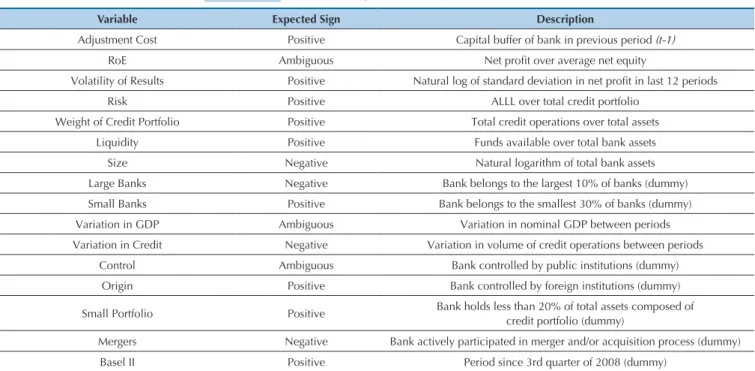
other studies were found that have used this variable. The set of variables described is detailed in Table 1, which also contains the respective signs expected.
Table 1 Expected signs for the dependent variables
Table 2 Descriptive Statistic for Variables Used in the Study
Variable Expected Sign Description
Adjustment Cost Positive Capital buffer of bank in previous period (t-1)
RoE Ambiguous Net proit over average net equity
Volatility of Results Positive Natural log of standard deviation in net proit in last 12 periods
Risk Positive ALLL over total credit portfolio
Weight of Credit Portfolio Positive Total credit operations over total assets
Liquidity Positive Funds available over total bank assets
Size Negative Natural logarithm of total bank assets
Large Banks Negative Bank belongs to the largest 10% of banks (dummy)
Small Banks Positive Bank belongs to the smallest 30% of banks (dummy)
Variation in GDP Ambiguous Variation in nominal GDP between periods
Variation in Credit Negative Variation in volume of credit operations between periods
Control Ambiguous Bank controlled by public institutions (dummy)
Origin Positive Bank controlled by foreign institutions (dummy)
Small Portfolio Positive Bank holds less than 20% of total assets composed ofcredit portfolio (dummy)
Mergers Negative Bank actively participated in merger and/or acquisition process (dummy)
Basel II Positive Period since 3rd quarter of 2008 (dummy)
Variables Frequency Average Standard Deviation VC Minimum Maximum
Buffer 4,670 2.5212 6.1603 2.4434 -2.1309 112.0055
RoE 4,653 0.0289 0.1163 4.0173 -3.1761 2.2325
Risk 4,670 0.0612 0.0963 1.5732 0.0000 1.0000
Size (Assets in R$1,000) 4,670 19,067,706 74,457,786 3,9049 12,424 935,009,463
GDP Growth 4,670 2.8231 15.4400 5.4691 -0.9908 107.0289
Portfolio Growth 4,653 0.1136 1.6023 14.1003 -1.0000 97.5100
Volatility 4,670 9.0960 2.0265 0.2228 0.0000 14.6346
Liquidity 4,670 0.4141 0.2425 0.5856 0.0001 0.9921
Weight of Portfolio 4,670 0.3885 0.2693 0.6932 0.0000 1.0344
Source: Developed by the authors.
Note. VC is the variation coefficient (standard deviation/average). Source: Developed by the authors.
In Table 2, the descriptive statistic for each of the variables used in the study can be observed.
Table 2 contains the descriptive statistics for the beha-vior of the variables in the study, with the exception of the dummy variables, in the sample of 121 in the period from 2001 to 2011.
he most dispersed behavior variables in the sample were portfolio growth, GDP growth, RoE, size (assets me-asured in monetary units), the regulatory capital bufer itself, and risk, which exhibited higher variation
3.3 Econometric Modeling
The econometric model used to analyze the beha-vior of banks’ capital buffers during the period analyzed was one with dynamic panel data, given the presence of a lagged dependent variable being an explanatory va-riable.
The estimation for the model was carried out as de-fined in Equation 1, based on the study carried out by Ayuso et al. (2004), in which capital buffers are deter-mined by the trade-off between the costs of holding ca-pital, bankruptcy, adjustment, and other variables that may have an influence over them.
where BUFi,t represents the capital bufer, BUFi,t-1 re-presents the adjustment cost, ROEi,t represents the cost of holding capital, RISKi,t represents the cost of bankruptcy, ωi,t represents other factors that may afect the capital bu-fer, as mentioned previously, and εi,t represents the
com-posed error term.
he parameters in Equation 1 were estimated by the Generalized Method of Moments (GMM), in accordance with the procedures from Arellano and Bover (1995), and Blundell and Bond (1998).
1
BUF
i,t= β
0BUF
i, t-1+ β
1ROE
i, t+ β
2RISK
i, t+ β
3ω
i, t+
ε
i, t4 RESULTS AND ANALYSES
4.1 Econometric Models Analyzed
The estimation of the econometric model represen-ted in Equation 1 was carried out in four models, each using a different set of variables, but all of which conver-ge with the support theory arguments. This procedure was adopted as a way of verifying the general model’s (Equation 1) degree of robustness with regard to the se-lected variables. The result found for the four models can be observed in Table 4.
Model 1 was based on the theoretical model from Ayuso et al. (2004), in which capital buffers are deter-mined by adjustment cost, the cost of holding capital, bankruptcy cost, bank size, and the economic cycle.
In Model 2, the economic cycle, represented by the Variation in GDP variable, is substituted by the demand for credit in the economy, represented by the Variation in Credit variable. As the use of the economic cycle se-eks to capture the behavior of capital buffers for all of the banks in the sample, without considering their par-ticular features, given that the Variation in GDP varia-ble only changes with time and not for individuals (time series), the demand for credit in the economy was used, represented by the Variation in Credit variable, which considers the particular features of a bank during the whole process.
In Model 3, the proxy used to verify the influence of bank size on capital buffers changed, with the Size varia-ble substituted by the dummy variavaria-bles Large Bank and Small Bank. The intention behind this alteration in the model was to observe the specific behavior of these two bank characteristics.
Model 4 used Model 2 as a base, adding the other variables presented previously, to observe the results al-together, and not using only the dummy variables Large
Bank and Small Bank.
4.2 Estimating Procedures and Tests
The estimation of the parameters used in the dy-namic panel model determined by the GMM System method in two stages, based on Arellano and Bover (1995), and Blundell and Bond (1998), which is an ex-tension of the original model from Arellano and Bond (1991). Estimation of the model in two stages is asymp-totically more efficient that in one stage, but can cau-se bias in the standard errors in small samples (Stolz & Wedow, 2011; Silva & Divino, 2012). To correct this bias in the standard errors the correction matrix pro-posed by Windmeijer (2005), known as the robust WC estimation, was used.
The autocorrelation test for the error terms indi-cated a first order autocorrelation, rejecting the null hypothesis of absence of autocorrelation for all of the models used, and indicated non rejection of the null hypothesis for second order autocorrelation for all of the models. The Sargan test, used to test the validity of the variables used as instruments (BUFt-1, RoE, and RISK), did not allow for rejection of the null hypothe-sis that all of the instruments are valid, thus indicating that the instrumental variables used are valid. The re-sults of the two tests demonstrated the validity of the specification and of the instruments used.
indi-viduals by means of a procedure based on the unitary root test for the individual average. The IPS considers it a null hypothesis that all of the panel set has a unita-ry root, with H0:ρi=0 for all of the individuals and, as an alternative hypothesis, that at least some individual does not have a unitary root, with Ha:ρi<0. In order to determine the numbers of lags in the test, the
proce-dure used by Ng and Perron (1995) was used, and an upper limit of four lags was adopted.
The IPS test was carried out in two functional ways, with a constant and without a trend, and with a cons-tant and with a trend, showing that the null hypothesis that all of the data series are not stationary was rejected with a 99% degree of certainty, as shown in Table 3.
Table 3 Unitary Root Test IPS
Variable With constant and without trend With constant and with trend Lags
Buffer -6.7307 -4.3452 4
(0.0000) (0.0000)
Note. p-value in brackets.
Source: Developed by the authors.
4.3 Analysis of the Results
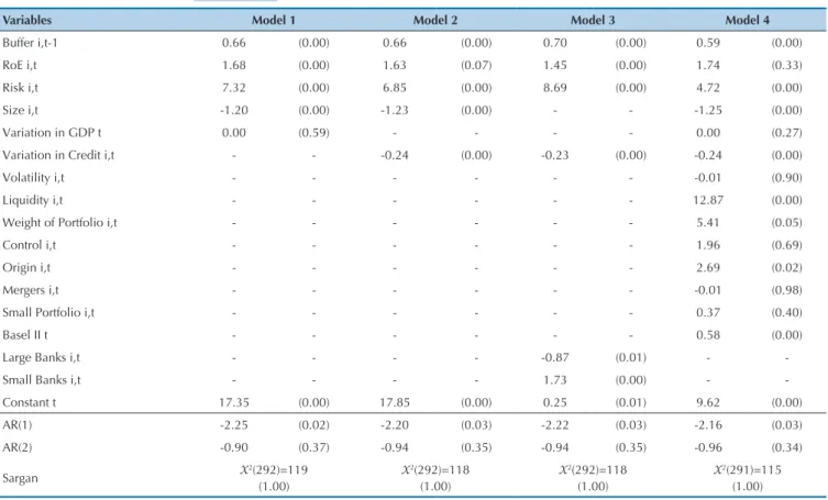
he results found for the four models can be observed in Table 4. he cost of bankruptcy, represented by the Risk variable, exhibited a positive sign and a 1% degree of signi-icance for all of the models. Its coeicient exhibited a small
variation in models 1, 2, and 3, and a greater variation in model 4, probably caused by the inclusion of more variables with bank risk proile characteristics. Based on the results found, it can be inferred that the Risk variable moved in the same direction as the capital bufers held by the banks.
Table 4 Estimation of GMM system model for capital buffers
Variables Model 1 Model 2 Model 3 Model 4
Buffer i,t-1 0.66 (0.00) 0.66 (0.00) 0.70 (0.00) 0.59 (0.00)
RoE i,t 1.68 (0.00) 1.63 (0.07) 1.45 (0.00) 1.74 (0.33)
Risk i,t 7.32 (0.00) 6.85 (0.00) 8.69 (0.00) 4.72 (0.00)
Size i,t -1.20 (0.00) -1.23 (0.00) - - -1.25 (0.00)
Variation in GDP t 0.00 (0.59) - - - - 0.00 (0.27)
Variation in Credit i,t - - -0.24 (0.00) -0.23 (0.00) -0.24 (0.00)
Volatility i,t - - - -0.01 (0.90)
Liquidity i,t - - - 12.87 (0.00)
Weight of Portfolio i,t - - - 5.41 (0.05)
Control i,t - - - 1.96 (0.69)
Origin i,t - - - 2.69 (0.02)
Mergers i,t - - - -0.01 (0.98)
Small Portfolio i,t - - - 0.37 (0.40)
Basel II t - - - 0.58 (0.00)
Large Banks i,t - - - - -0.87 (0.01) -
-Small Banks i,t - - - - 1.73 (0.00) -
-Constant t 17.35 (0.00) 17.85 (0.00) 0.25 (0.01) 9.62 (0.00)
AR(1) -2.25 (0.02) -2.20 (0.03) -2.22 (0.03) -2.16 (0.03)
AR(2) -0.90 (0.37) -0.94 (0.35) -0.94 (0.35) -0.96 (0.34)
Sargan X
2(292)=119
(1.00)
X2(292)=118
(1.00)
X2(292)=118
(1.00)
X2(291)=115
(1.00) Note. p-value in brackets.
Source: Developed by the authors.
he size of banks, represented by the Size variable, exhibited a negative sign and a 1% degree of signiicance for all of the models. For this variable, there was
he dummy variable Large Bank exhibited a negati-ve sign and a 1% degree of signiicance. he dummy va-riable Small Bank exhibited a positive sign and was also signiicant to a degree of 1%. he negative sign found for the dummy variable Large Bank is consistent with the sign found for the Size variable in models 1, 2, and 3, showing that the banks which comprised the largest 10% in terms of total assets held smaller capital bufers. he result found for the dummy variable Small Bank shows a complementary characteristic to the result found for the Size variable in models 1, 2, and 3, in which the small banks held larger capital bufers during the period.
he economic cycle, represented by the Variation in GDP variable, exhibited a positive sign, but was not sig-niicant for all of the models. Analyzing its sign alone, a positive sign would show that the economic cycle has a counter-cyclical behavior, and that an increase in capi-tal bufers is to be expected during economic growth, or oppositely, a reduction in capital bufers during an eco-nomic recession. As the coeicient found for the varia-ble was very close to zero, its 95% conidence interval varied between positive and negative values. hus, the results analysis for this variable was inconclusive, mea-ning it was not possible to make any inferences regarding the behavior of the economic cycle being pro-cyclical or counter-cyclical.
he Variation in Credit variable exhibited a negative sign and a 1% degree of signiicance in all of the models, and its estimated coeicients remained practically unal-tered. he result was as expected, given that an increase in the number of credit operations causes an increase in bank assets weighted by risk, providing evidence of movement in the opposite direction to the capital bufer variable.
he Volatility variable exhibited a negative sign, but was not signiicant to a 5% level of conidence. he sign found for this variable was the opposite to that expected, since it foresees that banks increase their capital bufers through retained earnings, given that the existence of high volatility in results would mean they were unable to rely on this source of funds, and need to hold larger capital bufers. he result found can be interpreted as the efect of volatility on banks’ ability to retain earnin-gs, given that volatility in results does not allow for the incorporation of earnings into the composition of their capital bufers. As the result for the variable was highly non signiicant (0,90), the analysis of its results was in-conclusive.
he Liquidity variable exhibited a positive sign and was signiicant to a degree of 1%. he sign found for this
variable was as expected, since the assets that compose it have little or no risk weighting. Another conclusion that can be inferred is that the fund raising carried out by banks, as a way of anticipating their capital needs, should have been applied in these liquid assets, given the impos-sibility of investing these funds in credit operations, at the time they are raised.
he Weight of Portfolio variable exhibited a positive sign and was signiicant to a degree of 5%. his variable is related to cost of bankruptcy for banks, demonstrating their risk proile. From the result found, it is inferred that the banks that apply a higher percentage of their assets in credit operations held larger capital bufers to cope with the underlying risk of their operations, with this variable being an ex ante measure of risk for Brazilian banks.
he dummy variable Control exhibited a positive sign, but was not signiicant to a degree of 10%. he sign exhibited by the variable shows that the banks controlled by public federal and state institutions held larger capital bufers than the banks controlled by private institutions. Given the non signiicance of the variable, the analysis of it was inconclusive.
he dummy variable Origin exhibited a positive sign and was signiicant to a degree of 5%. he sign of the va-riable was the result that was expected. his result makes it possible to infer that, as the Basel II principles were implemented by foreign countries a longer time ago, their managers behaved more actively with regards to risk and capital management, in adherence to the Pillar II concepts of Basel II.
he dummy variable Mergers exhibited a negative sign, but was not signiicant to a degree of 10%. he sign of the variable was compatible with what was expected, since it is assumed that the banks that took part in mer-ger and/or acquisition processes had an increase in their assets weighted by risk, thus consuming their capital bu-fers. As the result was highly non signiicant, the analy-sis of the variable was inconclusive.
he dummy variable Small Portfolio exhibited a posi-tive sign, but was not signiicant to a degree of 10%. he sign of the variable was as expected, but its analysis was inconclusive.
he dummy variable Basel II exhibited a positive sign and was signiicant to a degree of 1%. he sign of the variable was as predicted. his result allows it to be inferred that, with the adoption of the Basel II accord in Brazil, the banks implemented and streamlined their risk and capital management models, resulting in higher solvency monitoring, and, consequently, higher capital bufers being held.
5 FINAL REMARKS
This study sought to analyze the adequacy of the determining factors, proposed by the international li-terature, for holding regulatory capital buffers, for the
Alencar, L. S. (2011). Um exame sobre como os bancos ajustam seu Índice de Basileia no Brasil [Trabalho para discussão nº 251, p.
1-22]. Banco Central, Brasília, DF.
Araújo, L. A. D., Jorge, P. M., Neto, & Linhares, F. (2008). Capital,
risco e regulação dos bancos no Brasil. Pesquisa e Planejamento
Econômico, 38(3), 459-486.
Arellano, M., & Bond, S. (1991). Some tests of specification for panel data: Monte Carlo evidence and an application to employment
equations. The Review of Economic Studies, 58(2), 277-297.
Arellano, M., & Bover, O. (1995). Another look at the instrumental
variable estimation of error-components models. Journal of
econometrics, 68(1), 29-51.
Ayuso, J., Perez, D., & Saurina, J. (2004). Are capital buffers
pro-cyclical? Evidence from Spanish panel data. Journal of Financial
Intermediation, 13(2), 249–264.
Banco Central do Brasil (2012). Relatório de Estabilidade Financeira,
11(1). Retrieved on July 01, 2012, from http://www.bcb.gov.
br/?RELESTAB201203.
Baltagi, H. B. (2008). Econometric Analysis of Panel Data (4th ed.).
Chichester, West Sussex: John Wiley & Sons Ltd.
References
The international literature indicates adjustment cost, cost of holding capital, and bankruptcy cost as the main factors that determine capital buffers held. As well as these factors, the literature also mentions secondary factors such as size, economic cycle, and certain control variables.
With an aim to investigating whether such factors would be related to capital buffers being held in the case of Brazilian banks, an econometric model was formulated that was tested in four different ways, all composing dynamic data panels.
The result for the Adjustment Cost variable in-dicated a positive sign and significance in all of the models. The result found shows that, for the period analyzed, Brazilian banks exhibited high capital ad-justment costs, with no great variations in capital be-tween periods.
The RoE variable, describing the cost of holding capital, exhibited a positive sign, despite not being significant in all of the models, indicating that higher returns on capital can be used to increase banks’ capi-tal buffers. As the sign exhibited by the variable was positive in this study, it was not a good proxy for re-presenting the cost of holding capital, which should exhibit a negative sign.
Cost of bankruptcy also exhibited statistical signi-ficance for the Brazilian banks through the variables that were used as proxies – Risk (ALLL/credit portfo-lio), Liquidity (financial investments/total assets), and Weight of Portfolio (credit portfolio/total assets). The result showed that the Brazilian banks’ capital buffers moved in the same direction as the risk profile of their operations, increasing capital buffers when there is a greater risk profile, as expected.
With regards to size, it can be observed that the bigger the bank, the smaller its capital buffer, as was expected and consistent with the better investments and portfolio diversification hypothesis, and with the “too big to fail” hypothesis. The dummy variables Lar-ge Bank and Small Bank also showed that the larLar-gest banks held lower capital buffers and the small banks held larger capital buffers.
With relation to the economic cycle (variation in GDP), the results did not allow it to be stated whether behavior was pro-cyclical or counter-cyclical, given
the non significance of the results. With relation to demand for credit (Variation in Credit Portfolio), an inverse relationship was observed, indicating that the more credit was granted, the lower the buffer was, as was expected. This showed that the banks did not rai-se sufficient funds to cope with the risks of therai-se new operations, which caused a reduction in their capital buffers.
For the qualitative variables Control and Small Portfolio, it was not possible to draw any conclusions regarding their results, due to the non significance of them. With relation to the Origin variable, it was sho-wn that the foreign banks held larger capital buffers than the Brazilian banks, as was expected, suggesting the possibility of foreign managers behaving more ac-tively with regards to managing their capital.
With relation to the occurrence of mergers and ac-quisitions, a reduction in capital buffers was expected. The sign found was consistent with that expected, but without it being conclusive, given the non significance of the Mergers variable.
For the Basel II variable it is inferred that with the implementation of the Basel II accord, the banks came to hold a higher level of capital buffers, verified by the implementation and streamlining of risk and capital management models, resulting in greater monitoring of their solvency.
This paper contributes to studies of factors that in-fluence the determining of banks’ capital buffers, seen to be a poorly studied issue, mainly with regards to Brazilian banks. Moreover, the study also contributes to the field of Accounting and financial markets, assis-ting in understanding the structure of capital held by the banking sector, a segment that is generally exclu-ded from studies focused on capital structure.
Correspondence Address:
Vinícius Cintra Belém Banco do Brasil
SBS Ed. Sede III – 17º andar – CEP: 70.073-901 Brasília – DF – Brasil
Email: [email protected]
Berger, A. N., Herring, R. J., & Szegö, G. P. (1995). The role of capital
in financial institutions. Journal of Banking & Finance, 19(3),
393–430.
Bikker, J. A., & Metzemakers, P. A. J. (2007). Is bank capital
procyclical? A cross-country analysis. Kredit und Kapital, 40(2),
225–264.
Blundell, R. W., & Bond, S. R. (1998). Initial conditions and moment
restrictions in dynamic panel data Models. Journal of Econometrics,
87(1), 115-143.
Boucinha, M., & Ribeiro, N. (2007). Determinantes do excesso
de capital dos bancos portugueses. Relatório de Estabilidade
Financeira, Banco de Portugal. Lisboa.
Conselho Monetário Nacional (1999). Resolução nº 2.682, de 21 de dezembro de 1999. Retrieved on June 9, 2012 from http://www. bcb.gov.br/pre/normativos/busca/normativo.asp?tipo=res&ano=19 99&numero=2682.
Elizalde, A., & Repullo, R. (2007). Economic and regulatory capital in
banking: What is the difference? International Journal of Central
Banking, 3(3), 87-117.
Estrella, A. (2004). The cyclical behavior of optimal bank capital.
Journal of Banking & Finance, 28(6), 1469–1498.
Ferreira, R. A., Noronha, A. C., Tabak, B. M., & Cajueiro, D. O. (2010).
O comportamento cíclico do capital dos bancos brasileiros. Revista
Economia, 11(3), 671-690.
Fonseca, A. R., & González, F. (2010). How bank capital buffers vary across countries: The influence of cost of deposits, market power
and bank regulation. Journal of Banking & Finance, 34(4), 892-902.
Glantz, M (2007). Gerenciamento de riscos bancários: introdução a uma
ampla engenharia de crédito. Rio de Janeiro: Elsevier. Gropp, R., & Heider, F. (2010). The determinants of bank capital
structure. Review of Finance, 14(4), 587-622.
Im, K. S., Pesaran, M. H., & Shin, Y. (2003). Testing for unit roots in
heterogeneous panels. Journal of econometrics, 115(1), 53-74.
Jokipii, T., & Milne, A. (2008). The cyclical behaviour of European
bank capital buffers. Journal of Banking & Finance, 32(8),
1440–1451.
Jokipii, T., & Milne, A. (2011). Bank capital buffer and risk adjustment
decisions. Journal of Financial Stability, 7(3), 165-178.
Lindquist, K. G. (2004). Banks’ buffer capital: how important is risk.
Journal of International Money and Finance, 23(3), 493–513. Medeiros, O. R., & Pandini, E. J. (2007). Índice de Basileia no Brasil:
bancos públicos x privados. Revista de Educação e Pesquisa em
Contabilidade (REPeC), 1(2), 22-42.
Mehran, H., & Thakor, A. (2011). Bank capital and value in the
cross-section. Review of Financial Studies, 24 (4), 1019-1067.
Myers, S. C. (1984). The capital structure puzzle. Journal of Finance,
39(3), 575-592.
Ng, S., & Perron, P. (1995). Unit root tests in ARMA models with
data-dependent methods for the selection of the truncation lag. Journal
of the American Statistical Association, 90(429), 268-281. Peura, S., & Keppo, J. (2006). Optimal bank capital with costly
recapitalization. The Journal of Business, 79(4), 2163-2201.
Rime, B. (2001). Capital requirements and bank behaviour: Empirical
evidence for Switzerland. Journal of Banking & Finance, 25(4),
789-805.
Shrieves, R. E., & Dahl, D. (1992). The relationship between risk and
capital in comercial banks. Journal of Banking & Finance, 16(2),
439-457.
Silva, M. S. da, & Divino, J. A. (2012). Determinantes do capital
excedente na indústria bancária brasileira. Pesquisa e Planejamento
Econômico, 42(2), 261-293.
Stolz, S., & Wedow, M. (2011). Banks’ regulatory capital buffer and
the business cycle: Evidence for Germany. Journal of Financial
Stability, 7(2), 98–110.
Tabak, B. M., Fazio, D. M., & Cajueiro, D. O. (2011). The relationship between banking market competition and risk-taking: do size and capitalization matter? [Trabalho para discussão nº 261, p. 1-42].
Banco Central, Brasília, DF.
Tabak, B. M., Li, D. L., Vasconcelos, J. V. L., & Cajueiro, D. O. (2013). Do capital buffers matter? A study on the profitability and funding costs determinants of the Brazilian banking system [Trabalho para
discussão nº 333, p. 1-36]. Banco Central, Brasília, DF.
Tabak, B. M., Noronha, A. C., & Cajueiro, D. O. (2011). Bank capital buffers, lending growth and economic cycle: empirical evidence for
Brazil [Working Paper nº 4]. Banking for International Settlements,
Basel, Switzerland.
Vallascas, F., & Hagendorff, J. (2013). The risk sensitivity of capital requirements: evidence from an international sample of large
banks. Review of Finance, 17(6), 1947-1988.
Windmeijer, Frank. (2005). A finite sample correction for the
variance of linear efficient two-Step GMM estimators. Journal of