DISSERTATION DOUBLE UNIT TESTS IN THE PRESENCE OF STRUCTURAL BREAKS FRANCISCO ANTÓNIO TEIXEIRA MENDONÇA

MASTER OF SCIENCE IN

APPLIED ECONOMETRICS AND FORECASTING

MASTERS FINAL WORK

DISSERTATION

DOUBLE UNIT TESTS IN THE PRESENCE OF

STRUCTURAL BREAKS

FRANCISCO ANTÓNIO TEIXEIRA MENDONÇA

MASTER OF SCIENCE IN

APPLIED ECONOMETRICS AND FORECASTING

MASTERS FINAL WORK

DISSERTATION

DOUBLE UNIT TESTS IN THE PRESENCE OF

STRUCTURAL BREAKS

FRANCISCO ANTÓNIO TEIXEIRA MENDONÇA

Supervisor:

Professor Nuno Sobreira

i

DOUBLE UNIT TESTS IN THE PRESENCE OF

STRUCTURAL BREAKS

By Francisco Mendonça

We develop new statistical procedures aiming at accessing

the presence of exactly two unit roots in a time series, that may

have a single shift in its trend function, at a known or unknown

date. The test statistics have a non-standard distribution based on

ii

iii

Acknowledgments

I am grateful to Professor Nuno Sobreira for continuously challenging me to go further,

and for sharing his knowledge with me. Without him, this work would not be possible.

I also appreciate the valuable inputs from Professor João Nicolau, which helped to

iv

Abstract

The work presented concerns the field of unit root testing, allowing for the

possibility of changes in the trend function of a time series. Two tests were designed for

the null hypothesis of exactly two-unit roots, one for the case of a known change date,

and another for the more likely case of an unknown changepoint. Each test statistic

follows a non-standard distribution, which are based on functions of Wiener processes.

The percentiles for both distributions were obtained via Monte Carlo simulation. Both

tests were applied to several economic variables, and the results suggest that the double

unit root hypothesis is a suitable candidate to explain the persistence of the innovations

guiding many of those variables.

v

JEL: C12, C22.

Resumo

O trabalho que se apresenta, centra-se no campo dos testes de raiz unitária,

permitindo a existência de alterações na função de tendência de uma série temporal.

Foram construídos dois testes para a hipótese nula de exatamente duas raízes unitárias,

um para o caso de data de quebra conhecida, e outro para o cenário mais provável de

uma data de quebra desconhecida. Ambas as estatísticas de teste seguem uma

distribuição não convencional, baseada em processos de Wiener. Os percentis destas

distribuições foram obtidos via simulação de Monte Carlo. Ambos os testes foram

aplicados a várias variáveis económicas e os resultados sugerem que a hipótese de duas

raízes unitárias é uma boa candidata para explicar a persistência das inovações em

algumas destas séries.

Palavras-Chave:

Contents

Acknowledgments ... iii

Abstract ... iv

Resumo ... v

List of Tables ... vi

List of Figures ... vii

1 Introduction ... 1

2 Literature Review... 3

3 The Double-Unit Root Process and its Characteristics ... 5

4 The Trend Break Model ... 7

5 Conventional double unit root tests under a break in trend ... 9

6 Double unit root tests in the presence of a trend break ... 14

6.1 Known Break Date ... 14

6.2 Unknown Break Date ... 18

6.3 Rejecting the Null Hypothesis ... 22

7 Size and Power Simulations ... 22

8 Empirical Applications ... 27

9 Conclusions ... 33

References ... 35

A Data Appendix ... 38

vi

List of Tables

Table I: Null Rejection Probabilities. Hasza-Fuller Test ... 10

Table II: Selected Percentiles of the Asymptotic Distribution of _{𝐹𝝆𝑖𝜆} ... 18

Table III: Selected percentiles of the distribution of _{𝑠𝑢𝑝𝜆 ∈ 𝛬𝐹𝝆𝑖𝜆} ... 21

Table IV: Null Rejection Probabilities – Known Changepoint Test ... 23

Table V: Null Rejection Probabilities – Unknown Changepoint Test ... 24

Table VI: Tests for the Double Unit Root Null Hypothesis ... 29

Table VII: Tests for the Double Unit Root Null Hypothesis - Revised ... 31

vii

List of Figures

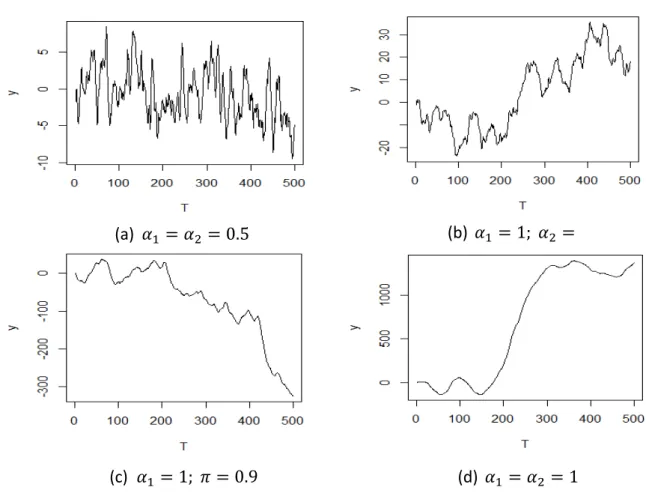
Figure 1 – Simulated paths for the process given in equation (1) with _{et~iid N0, 1} ... 7

Figure 2 Size (left) and Power (right) as a function of the number of changepoints for Model A ... 25

Figure 3 - Size as a function of the break parameters. Model A (left) and Model B (right) ... 25

1

1 Introduction

Testing for unit roots has received great attention over the latest decades, and

has now become a standard procedure in time series analysis. Some of the most

important consequences of the unit root hypothesis are the permanent effect of shocks

on the long-run behaviour of a time series, its disruptive effect on conventional

statistical inference, forecasting and properties of estimators, namely the Ordinary Least

Squares (OLS) estimator.

Perron (1989) made a very important contribution to the unit root literature as he

emphasized the empirical relevance of breaks in the trend function of economic and

financial data, and its effect on the OLS estimators and unit root tests. Perron proved

that the presence of structural breaks dramatically decreased the power of the Dickey

Fuller (DF) and Augmented Dickey Fuller (ADF) test statistics. However, Perron’s

proposed test statistic requires a priori knowledge of the eventual date at which the break occurs. This was considered an important limitation and several authors sought to

develop unit root tests that do not assume a known break date (Zivot & Andrews, 1992,

and Perron, 1997, for example). Others, developed unit root test statistics which allow

more than one changepoint in the trend, such as Lumsdaine & Papell (1997).

However, the focus remained on testing for exactly one unit root, and rule out

the possibility of more unit roots. In applied work, there have been cases of series which

seem to behave according to a double unit root process such as price series, wages,

stock variables and population (see, Haldrup, 1998, for example). The conventional

2

(1987) and Sen & Dickey (1987). These authors propose tests for the null hypothesis of

two-unit roots but without permitting structural breaks in the deterministic components.

The purpose of this thesis is to extend double unit root testing procedures

allowing for the presence of breaks in the data. Instead of assuming exactly one unit

root under the null hypothesis, it will be assumed two unit roots. Two test statistics are

considered. One is valid under the assumption of a known break date and is shown to

have a non-standard limiting distribution and its percentiles are obtained through Monte

Carlo simulations and provided in this thesis. The second statistic relaxes the known

break date assumption and follows the method of Zivot & Andrews (1992) to propose

an endogenous change point version of the test. The hypothesis of an unknown break

date implies the need for an estimate for the break date, which is taken to be the one that

gives the strongest evidence against the null hypothesis. It is shown that the asymptotic

distribution of the test statistic is non-standard and again its percentiles are obtained

through Monte Carlo simulations and provided in this thesis.

The dissertation is organized as follows. Section 2 reviews the existing literature

on the topic of unit root testing with structural changes in the deterministic component.

Section 3 briefly addresses double-unit root processes and its characteristics, as well as

some important limiting results. Section 4 addresses the trend break model. Section 5

explores the effect of structural breaks on the Hasza & Fuller test and derives the

limiting distribution of the OLS estimator under the hypothesis of stationarity and

exactly one-unit root, when structural changes are present, but ignored. In Section 6 the

test statistics are presented and motivated, and its limiting distributions are derived as

well as the simulated percentiles. Section 7 analyses empirical power and size through

3

alternatives, including different pairs of autoregressive roots and more complex

deterministic functions. In Section 8, the tests are applied to several time series, where

we explore and comment on the results. Section 9 is reserved for the concluding

remarks and suggestions for future research. The proofs of the theorems can be found in

the Mathematical Appendix.

2 Literature Review

This dissertation develops tests for two unit roots in an univariate time series that

can be used when there are structural breaks in the trend function.

After the seminal paper of Nelson & Plosser (1982), it was believed that many

macroeconomic time series were well described by a unit root process. However, at the

time, the existing tests for the null hypothesis of exactly one unit root were based on

strict assumptions, namely, parameter constancy of the deterministic components. Yet,

we can identify a number of significant events that seem to have altered the path of

several economic variables, such as the Great Crash (1929), the First and Second World

Wars (1914-1919 and 1939-1945, respectively), the Oil Price Shock (1973), and more

recently, the Financial Crisis (2007) that started with the bankruptcy of Lehman

Brothers. These events, if not modelled, can potentially invalidate any inference based

on unit root tests.

This means that unit roots and structural breaks cannot be treated independently.

Perron (1989) made the first breakthrough, showing how structural changes impacted

unit root tests. He proposed a test based on an augmented Dickey-Fuller regression that

sought to eliminate the effect of the structural change. However, the test was based on

4

many time series, studied by Nelson & Plosser (1982), that were first taught to exhibit a

unit root, could instead be described by an I(0) process around a changing trend

function.

The paper of Perron (1989) marked the beginning of a new strand in the

literature of unit root testing. From that point onwards many authors worked to develop

new tests which allowed for an unknown changepoint, whilst other studied the effect of

using wrong break dates. For example, Zivot & Andrews (1992) developed the widely

used _{inf 𝑡} test, which searches for the break date that maximizes the likelihood of

observing the alternative hypothesis. Perron (1997) presents a more complete test that

allows for a breakpoint under the null and alternative hypothesis. Other authors opted to

explore the behaviour of Perron’s (1989) test, such as Montañés (1997), which revealed

that an erroneous choice of the changepoint used in Perron’s 𝑡 test caused a significant

loss in power in small samples

More recent examples of robust unit root tests include Carrion-i-Silvestre, Kim

& Perron (2009) for their GLS-based unit root test that allows for multiple breaks both

under the null and alternative hypothesis; Harvey, Leybourne & Taylor (2013) which

propose minimum DF statistics in the possible presence of multiple breaks; Cavaliere et

al. (2011) present a robust unit root test under multiple possible changepoints and non-stationary volatility, using bootstrapped minimum DF test statistics.

Nevertheless, robust tests that allow for more than one unit root under the null

hypothesis have not been developed. Since the existing tests allow for exactly one unit

root under the null hypothesis, if a time series process exhibits more roots equal to

5

The literature for two unit roots is scarcer. Nonetheless, there are some

important contributions, namely Hasza & Fuller (1979) for an F-test which allows to

test the restrictions imposed by the two unit roots; Dickey & Pantula (1987) for a

sequential procedure based on 𝑡-statistics which allows for testing multiple unit roots,

starting from the highest number of roots and testing down; Sen & Dickey (1987)

proposed a _𝑡 test based on a symmetric OLS estimator. More recently, Haldrup (1994)

and Shin & Kim (1999) develop semi-parametric tests for two unit roots. However,

double unit root tests carry additional complexity, particularly when concerning the

initial conditions. Rodrigues & Taylor (2003) explore the role of the initial conditions

on the double unit roots tests, and find that the Hasza-Fuller F test and Sen-Dickey t

test, are not invariant to the starting values and that the limit distributions depend on the

demeaning method used.

Although tests for two unit roots have been developed, none is robust to

structural changes in the deterministic function, thus, this dissertation seeks to address

this issue, and proposes two tests that allow for that possibility.

3 The Double-Unit Root Process and its Characteristics

Consider the following dynamic process for _{𝑦𝑡}, without any type of

deterministic component:

(1 − 𝛼1𝐿)(1 − 𝛼2𝐿)𝑦𝑡 = 𝑒𝑡, 𝑒𝑡~𝑖𝑖𝑑 (0, 𝜎2_{) (1)}

It is well known that when _{𝛼1 = 1} (or _{𝛼2 = 1)} and _{|𝛼2| < 1} (or _{|𝛼1| < 1)} we have that

{𝑦𝑡} has one unit root. The idea of the DF and ADF type of statistics is to test this

6

roots. However, when a second unit root is allowed, the statistical framework is more

complex. In particular, when a test for two unit roots is performed in _{𝑦𝑡}, the

alternative hypothesis is not necessarily a stationary process as in DF and ADF, because

under the alternative hypothesis, the process can either be a unit root process (_{𝛼1 = 1,}

|𝛼2| < 1 or _{|𝛼1| < 1, 𝛼2 = 1}), or I(0) (_{|𝛼1| < 1, |𝛼2| < 1)} process. Naturally it can

also be an explosive process (_{|𝛼2| > 1} or _{|𝛼1| > 1} or both) but we do not consider this

possibility in this thesis. A second source of additional complexity is the effect of the

starting values. To see this, take equation ₍₁₎ with _{𝛼1 = 𝛼2 = 1} and solve recursively,

denoting the starting values by 𝑦0 and 𝑦−1, yielding:

𝑦𝑡 = 𝑦0+ (𝑦0− 𝑦−1)𝑡 + ∑𝑡𝑗=1∑𝑗𝑘=1𝑒𝑘 (2)

This equation explicitly shows that, even without adding any deterministic component

to the right-hand side of equation ₍₁₎, the starting values generate a linear trend if

𝑦−1 ≠ 𝑦0. Thus, in order for our tests to be invariant to these starting values we must

introduce a linear trend to the test equations.

Another characteristic of double integrated processes is its smoothness, when

compared to I(0) and one-unit root processes as it can be observed in Figure 1. This is a

7

4 The Trend Break Model

In this thesis, we assume that the time series under analysis, denoted as _𝑦𝑡, is a

realization of the following time series process (DGP):

𝑦𝑡 = 𝜷𝒊′𝒛𝒕𝒊(𝜆) + 𝑥𝑡, 𝑡 = 1, … , 𝑇, 𝑖 = 𝐴, 𝐵, 𝐶 (3)

where

𝒛𝒕𝑨(𝜆) = (1, 𝑡, 𝐷𝑈𝑡(𝜆))′, 𝒛𝒕𝑩(𝜆) = (1, 𝑡, 𝐷𝑇𝑡(𝜆))′, 𝒛𝒕𝑪(𝜆) = (1, 𝑡, 𝐷𝑈𝑡(𝜆), 𝐷𝑇𝑡(𝜆))′ (4)

and

𝜷𝑨′_{= (𝜇}𝐴_{, 𝛿}𝐴_{, 𝜇}

𝑏𝐴)′, 𝜷𝑩′ = (𝜇𝐵, 𝛿𝐵, 𝛿𝑏𝐵)′, 𝜷𝑪′ = (𝜇𝐶, 𝛿𝐶, 𝜇𝑏𝐶, 𝛿𝑏𝐶)′

(a) 𝛼1 = 𝛼2 = 0.5 (b) 𝛼₁ = 1; 𝛼₂ =

0.5

(c) 𝛼1 = 1; 𝜋 = 0.9 (d) 𝛼1 = 𝛼2 = 1

8

with _{𝐷𝑈𝑡(𝜆) = 1(𝑡 > 𝑇𝑏)} and _{𝐷𝑇𝑡(𝜆) =1(𝑡 > 𝑇𝑏)(𝑡 − 𝑇𝑏)}. Here ₁₍ . _{) is the indicator}

function and _{𝑇𝑏= ⌊𝜆𝑇⌋} the break date with _{⌊. ⌋} denoting the integer part.

In words, the underlying process is generated as the sum of a deterministic

(_𝜷𝒊′_𝒛 𝒕

𝒊_{(𝜆), 𝑖 = 𝐴, 𝐵, 𝐶) and a stochastic component (𝑥}

𝑡). We allow the deterministic

component to contain a linear trend and we assume that an exogenous shock may occur

at period _𝑇𝑏 and cause a structural break in the process. In general, such a break is

modelled as a permanent change in the parameters of the trend function after its

occurrence. This justifies the functional form of the deterministic part of (3) and the fact

that equation (3) is referred in the literature as the “trend break model” (see, for

example, Harvey et al., 2009). In particular, we consider three possible formulations of

the trend break model: under Model A (i=A) and Model B (i=B) the exogenous shock may cause either a level shift or a slope shift, respectively. Under Model C (i=C), we allow for a simultaneous level and slope shift as a consequence of the break.

The stochastic component is assumed to follow an _𝐴𝑅(2) process for simplicity:

(1 − 𝛼1𝐿)(1 − 𝛼2𝐿)𝑥𝑡 = 𝑒𝑡, 𝑒𝑡~𝑖. 𝑖. 𝑑 (0, 𝜎2_{) (5)}

The purpose of this thesis is to propose statistical procedures to test the presence of two

unit roots in the process generating _𝑦𝑡. Here the relevant null hypothesis is _{𝐻0: 𝛼1 =}

𝛼2 = 1 and the alternatives may be either one-unit root

(𝛼𝑗 = 1 ∧ |𝛼𝑠| < 1, 𝑗 = 1,2; 𝑠 = 1,2; 𝑗 ≠ 𝑠) or no unit roots (|𝛼1| < 1 ∧ |𝛼2| < 1).

We highlight that, to our knowledge, this is the first statistical testing procedure for the

9

5 Conventional double unit root tests under a break in trend

As remarked in the previous section, the interest of this thesis lies in testing the

null hypothesis of I(2)ness in _𝑦𝑡. A number of statistical procedures have been proposed

in the literature to test for the presence of two unit roots as mentioned in Section 2.

However, all of these tests ignore the problem of structural breaks in the trend. Hence,

to motivate this thesis a natural question to ask is: what are the consequences for

conventional double unit root tests in terms of size and power when breaks in trend are

present in the DGP?

For illustration, we study the behaviour of the Hasza & Fuller test (henceforth

HF). Consider the auxiliary regression of the HF test:

∆2_{𝑦𝑡 = 𝜇}∗_{+ 𝛿}∗_{𝑡 + 𝜌1𝑦𝑡−1+ 𝜌2∆𝑦𝑡−1+ 𝑒𝑡 (6)}

Notice that this equation is nested in the statistical framework described by equations

(3) and (5) with _{𝜇𝑏 = 𝛿𝑏 = 0}, i.e., without a break in trend. In particular, _𝜇∗ ₌ (1 − 𝛼1)(1 − 𝛼2)𝜇 + (𝛼1+𝛼2)𝛿 − 2𝛼1𝛼2𝛿, _𝛿∗ _{= (1 − 𝛼1)(1 − 𝛼2)𝛿}, _{𝜌1 =}

−(1 − 𝛼1)(1 − 𝛼2), _{𝜌2 = 𝛼1𝛼2− 1.} Given that _{𝑦𝑡~𝐼(2)} iff _{𝛼1 = 𝛼2 = 1}, the double

unit root null hypothesis is _{𝜌1 = 𝜌2 = 0}. According to HF, such restrictions are tested

with an F-type statistic which follows a non-standard asymptotic distribution under the

null. The critical values are well known and can be obtained, for example, from Table

10.2 of Patterson (2011).

To assess the small sample effect of structural breaks on the properties of the HF

test, a Monte Carlo experiment is presented. First, 5.000 replications of _{𝑦𝑡𝑖_} for _{𝑖 =}

𝐴, 𝐵 of length 150 are generated, setting _{𝜆 = 1/2}, then the empirical size and power of

10

𝛼1 = 1, 𝛼2 = 0.8, empirical power is computed. For the case 𝛼1 = 𝛼2 = 1, empirical

test size is computed. In all calculations, the test equation is (6), and the null hypothesis

tested is _{𝜌1 = 𝜌2 = 0}.

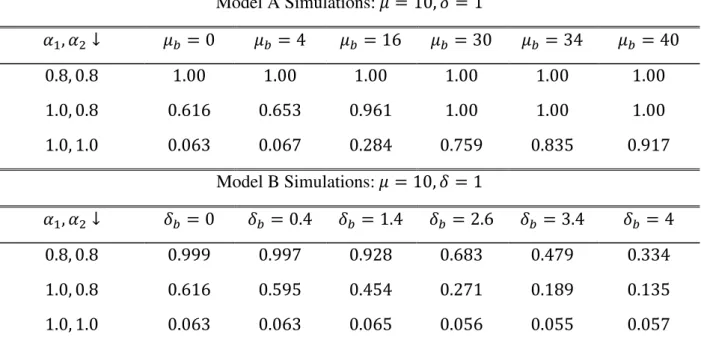
Table I: Null Rejection Probabilities. Hasza-Fuller Test

Model A Simulations: _{𝜇 = 10, 𝛿 = 1}

𝛼1, 𝛼2 ↓ 𝜇𝑏= 0 𝜇𝑏= 4 𝜇𝑏= 16 𝜇𝑏= 30 𝜇𝑏= 34 𝜇𝑏 = 40

0.8, 0.8 _{1.00 1.00 1.00 1.00 1.00 1.00}

1.0, 0.8 0.616 0.653 0.961 1.00 1.00 1.00

1.0, 1.0 0.063 0.067 0.284 0.759 0.835 0.917

Model B Simulations: 𝜇 = 10, 𝛿 = 1

𝛼1, 𝛼2 ↓ 𝛿𝑏 = 0 𝛿𝑏 = 0.4 𝛿𝑏 = 1.4 𝛿𝑏 = 2.6 𝛿𝑏= 3.4 𝛿𝑏 = 4

0.8, 0.8 _{0.999 0.997 0.928 0.683 0.479 0.334}

1.0, 0.8 0.616 0.595 0.454 0.271 0.189 0.135

1.0, 1.0 0.063 0.063 0.065 0.056 0.055 0.057

Table I shows that when the true process has solely a level shift (Model A), the

HF test becomes oversized and such an effect becomes more severe with the magnitude

of the break. The empirical power of the test also increases apparently as a result of the

size distortion. When the true process is Model B (only a break in the slope of the

trend), the opposite happens, power is significantly reduced for higher values of _𝛿𝑏 but

the size remains almost unchanged and close to the 5% level. Lastly, the simulations for

Model C (simultaneous level and slope shift) were not presented because the pattern

followed by power and size depend on which effect dominates the other. If _𝜇𝑏 is

significantly higher relative to _𝛿𝑏, then results from Model A apply, whilst the opposite

11

OLS estimators _𝝆̂𝑖 _{= (𝜌̂1}𝑖_{, 𝜌̂2}𝑖₎′_{𝑓𝑜𝑟 𝑖 = 𝐴, 𝐵, 𝐶} in equation (6), under the alternative

hypotheses that _{𝑥𝑡} is stationary and I(1).

Theorem 1: Let _{𝑦𝑡} be generated by model _{𝑖 = 𝐴, 𝐵, 𝐶,} according to equation (3).

Suppose we estimate equation (6), neglecting the level/slope shift. Then, as _{𝑇 → ∞}:

(1) Under the alternative hypothesis that _{|𝛼𝑠| < 1 , 𝑠 = 1,2}:

(a) Under Model A

(𝑎. 1) √𝑇(𝜌̂1− 𝜌1) →𝑑 𝑁[0, 2𝜎2𝜏] (𝑎. 2) √𝑇(𝜌̂2− 𝜌2) →𝑑 _{𝑁[0, 𝜎}2_𝜏]

Where

𝜏 = (−3𝜆4+ 6𝜆3− 4𝜆2+ 𝜆)𝜇𝑏2+ 𝛾0

(𝛾02− 𝛾12) + ((12𝜆3− 6𝜆4− 8𝜆2+ 2𝜆)𝛾0+ (6𝜆4− 12𝜆3+ 8𝜆2 − 2𝜆)𝛾1)𝜇𝑏2

(b) Under Models B and C

(𝑏. 1) 𝑇32(𝜌̂₁− 𝜌₁) →𝒅 𝑁[0, 𝜎2𝜃₁]

(𝑏. 2) √𝑇(𝜌̂2− 𝜌2) →𝒅 𝑁[0, 𝜎2𝜃2]

Where 𝜃1 = [𝑽]−1

3,3 𝜃2 = [𝑽]−1

4,4

Where _[𝑽]−1 is the inverse of the matrix _𝑽given by:

𝐕 =

[

1 1₂ 1_{2 𝛿}𝑏(1 − 𝜆)2 _{𝛿𝑏(1 − 𝜆)}

1 2

1 3

1

6 (1 − 𝜆)(2𝜆2𝛿𝑏− 4𝜆𝛿 + 2𝜆)

1

2 𝛿𝑏(1 − 𝜆)2 1

2 𝛿𝑏(1 − 𝜆)2 1

6 (1 − 𝜆)(2𝜆2𝛿𝑏− 4𝜆𝛿 + 2𝜆) 1

6(1 − 𝜆)(2𝜆2𝛿𝑏− 4𝜆𝛿 + 2𝜆)

1

12 (2)

(3) Under the hypothesis of exactly one-unit root in _{𝑦𝑡}

(c) Under Model A

Since the stochastic trend dominates the level shift, the asymptotic distributions are invariant to the break.

(d) Under Models B and C

(𝑑. 1) 𝑇32(𝜌̂1𝑖 − 𝜌₁𝑖) →𝑝 𝜃−1(𝐺1− 𝐺2) (𝑑. 2) √𝑇(𝜌̂2𝑖 − 𝜌2𝑖) →𝑝 𝜃−1(𝐺3− 𝐺4)

For 𝑖 = 𝐵 𝑜𝑟 𝐶

Where:

(1) 𝜃 =_{12 𝛿}1 𝑏2(𝜆 − 1)3(4𝛾0− 𝜆𝛿𝑏2(12𝜆6− 24𝜆5+ 15𝜆4− 15𝜆3 + 24𝜆2− 16𝜆 + 4))

(2) G1 = (𝛾0−𝜆𝛿𝑏2(3𝜆3− 6𝜆2+ 4𝜆 − 1))

× (𝜎𝛿𝑏(𝜆3_{− 𝜆}2_{− 2𝜆 + 2)𝑊(1) − 𝜎𝛿𝑏(1 − 𝜆)𝑊(𝜆)}

− 𝜎𝛿𝑏(∫ 𝑊(𝑟)𝑑𝑟 1

𝜆 + (𝜆 − 1)

2_{(1 + 2𝜆) ∫ 𝑊(𝑟)𝑑𝑟}1

0 ))

(3) G2 =1_{2 𝜆}2_𝛿

𝑏2(𝜆 − 1)2(2𝜆 − 1)

× (𝜎(𝛿𝑏(2 + 2𝜆 − 3𝜆2_{) − √𝛾0 )𝑊(1) − 𝛿𝑏𝜎𝑊(𝜆) − 6𝜆(1 − 𝜆)𝛿𝑏𝜎 ∫ 𝑊(𝑟)𝑑𝑟}1

0 )

(4) G3 =1_{6 𝛿}𝑏2(𝜆 − 1)2(3𝜆2− 6𝜆3)

× (𝜎𝛿𝑏(𝜆3_{− 𝜆}2_{− 2𝜆 + 2)𝑊(1) − 𝜎𝛿𝑏(1 − 𝜆)𝑊(𝜆)}

− 𝜎𝛿𝑏(∫ 𝑊(𝑟)𝑑𝑟 1

𝜆 + (𝜆 − 1)

2_{(1 + 2𝜆) ∫ 𝑊(𝑟)𝑑𝑟}1

0 ))

(5) G4 =1_{6 𝛿}𝑏2(𝜆 − 1)2(3𝜆2− 6𝜆3)

× (𝜎(𝛿𝑏(2 + 2𝜆 − 3𝜆2) − √𝛾0 )𝑊(1) − 𝛿𝑏𝜎𝑊(𝜆) − 6𝜆(1 − 𝜆)𝛿𝑏𝜎 ∫ 𝑊(𝑟)𝑑𝑟 1

0 )

13

Part (1) of Theorem 1 establishes that, under Model A, both estimators are

normally distributed, with asymptotic variance depending on the parameters _𝜇𝑏 and

𝜆. However, in small samples, the estimators are increasingly biased as _𝜇𝑏 grows, as can

be inferred from Table I. For Models B and C, the limiting distribution is also Normal,

with asymptotic variance as a function of _𝛿𝑏. From Table I, we find that in small

samples both estimators are biased towards zero zero, when _𝛿𝑏 grows. For models B

and C, the rate of converge of _𝜌̂1(_𝑇32) is higher than the common √𝑇, due to the fact

that the slope change _{(𝐷𝑇𝑡)} is present in the DGP but neglected in the test regression.

For the second part of the theorem, for Models B and C, the limiting distribution

of the OLS estimator depend on the slope shift parameter and the break fraction.

According to the simulations in Table I, for a given break fraction, both distributions

concentrate around zero when the slope shift parameter increases. The result for Model

A is not presented because the limiting distribution is not affected by the break

parameters, since the stochastic trend asymptotically dominates a level shift. However,

the small sample distribution clearly depends on these parameters, as can be seen from

Table I.

To sum up, changes in the deterministic component affect the outcome of the HF

test. The need for a consistent testing strategy follows from the results so far. For

Models B and C, the problem is the low power against stationary, and single unit root

alternatives, whilst for Model A it is a size problem. In fact, considering Model A, the

test will always reject the null hypothesis for a sufficiently large shift, thus leading to

the conclusion that the underlying process has less than two unit roots, when in fact it

14

shift in its level. Therefore, inference based on the simple Hasza-Fuller test cannot lead

to any valid conclusion. A similar argument holds for Models B and C.

6 Double unit root tests in the presence of a trend break

In this section, we present alternative testing procedures aimed at solving the

problems considered in the previous section. First, the Hasza-Fuller test is extended to

the case of a known break date. The methodology is similar to Perron (1989). Then a

test allowing for a break at an unknown date is devised. This test is closely related to the

𝑖𝑛𝑓 − 𝑡 test of Zivot & Andrews (1992).

6.1 Known Break Date

In this section we closely follow Perron (1989).

Consider the following modified test regression for Model C, where the dummy

variables are included:

𝑦𝑡 = 𝜇 + 𝛿𝑡 + 𝜇𝑏𝐷𝑈𝑡+ 𝛿𝑏𝐷𝑇𝑡+ 𝑥𝑡

(1 − 𝛼1𝐿)(1 − 𝛼2𝐿)𝑥𝑡 = 𝑒𝑡~𝑖. 𝑖. 𝑑 (0, 𝜎2)

These equations can be combined, and after suitable transformations we arrive to:

∆2_{𝑦𝑡 = 𝜇}∗_{+ 𝛿}∗_{𝑡 + 𝜃1𝐷𝑇}

𝑡+ 𝜃2𝐷𝑈𝑡+ 𝜃3∆𝐷𝑈𝑡+ 𝜃4∆2𝐷𝑈𝑡+ 𝜌1𝑦𝑡−1+ 𝜌2∆𝑦𝑡−1+ 𝑒𝑡

(7)

Where, _𝜇∗ _{= (1 − 𝛼1)(1 − 𝛼2)𝜇 + (𝛼1+𝛼2)𝛿 − 2𝛼1𝛼2𝛿}, _𝛿∗ _{= (1 − 𝛼1)(1 − 𝛼2)𝛿},

𝜃1 = (1 − 𝛼1)(1 − 𝛼2)𝛿𝑏, _{𝜃2 = (1 − 𝛼1)(1 − 𝛼2)𝜇𝑏+ (2 − 𝛼1 − 𝛼2)𝛿𝑏}, _{𝜃3 =}

(2 − 𝛼1− 𝛼2)𝜇𝑏+ 𝛼1𝛼2𝛿𝑏, 𝜃4 = 𝛼1𝛼2𝜇𝑏, 𝜌1 = −(1 − 𝛼1)(1 − 𝛼2), 𝜌2 = 𝛼1𝛼2− 1.

15

The OLS estimator of equation (7) attains exact invariance to the break parameters,

thus, that equation should be used to test the null hypothesis _{𝜌1 = 𝜌2 = 0}. However, the

following regression is asymptotically equivalent to (7):

∆2_{𝑦𝑡 = 𝜇}∗_{+ 𝛿}∗_{𝑡 + 𝜃1𝐷𝑇}

𝑡+ 𝜃2𝐷𝑈𝑡+ 𝜌1𝑦𝑡−1+ 𝜌2∆𝑦𝑡−1+ 𝑒𝑡

This is because _{∆𝐷𝑈𝑡} and _∆2_𝐷𝑈𝑡 are pulse dummies, and thus, _𝑜𝑝(1).

Hence, we can derive the limiting distribution of the test statistic with the reduced

equation.

Additionally, in empirical applications it might be needed to include lagged

second differences to equation (7) to account for the presence of serial correlation in the

error term _𝑒𝑡.

In the following theorem, we study the limit distributions of the test statistic

𝐹_𝝆̂𝑖_{(𝜆) from equation (7):}

Theorem 2: Let _{𝑦𝑡} be generated according to equation (3). Additionally, let 𝐹_𝝆̂𝑖_(𝜆)

denote the statistic used for testing the nullity of both _𝜌1𝑖 and _𝜌2𝑖 in equations ₍₇₎ for _{𝑖 =}

𝐴, 𝐵, 𝐶. Then, under the null hypothesis that 𝜌1 = 𝜌2 = 0, as 𝑇 → ∞:

(𝑎) 𝐹𝜌̂𝑖(𝜆) →𝑑 (2𝑆𝑖)−1𝐴𝑖

Where

𝐴𝑖 = (𝜂2𝑖(𝜆)[𝜉1𝑖(𝜆)]2− 2𝜂3𝑖(𝜆)𝜉1𝑖(𝜆)𝜉2𝑖(𝜆) + 𝜂1𝑖(𝜆)[𝜉2𝑖(𝜆)]2)

𝑆𝑖 = (𝜂1𝑖(𝜆)𝜂2𝑖(𝜆) − [𝜂3𝑖(𝜆)]2)

16

Where:

𝜉1𝑖(𝜆) = {∫ Υ1𝑑𝑊(𝑟)

1

0 − ∫ 𝒁

𝒊_{(𝜆, 𝑟)}′_{𝑑𝑊(𝑟) (∫ 𝒁}1 𝒊_{(𝜆, 𝑟)𝒁}𝒊_{(𝜆, 𝑟)}′_𝑑𝑟

0 )

−1

∫ 𝒁1 𝒊_{(𝜆, 𝑟)} 0

1

0 Υ1𝑑𝑟}

𝜉2𝑖(𝜆) = {∫ Υ2𝑑𝑊(𝑟) 1

0 − ∫ 𝒁

𝒊_{(𝜆, 𝑟)}′_{𝑑𝑊(𝑟) (∫ 𝒁}1 𝒊_{(𝜆, 𝑟)𝒁}𝒊_{(𝜆, 𝑟)}′_𝑑𝑟

0 )

−1

∫ 𝒁1 𝒊_{(𝜆, 𝑟)} 0

1

0 Υ2𝑑𝑟}

𝜂1𝑖(𝜆) = ∫ {Υ1− 𝒁𝒊(𝜆, 𝑟)′(∫ 𝒁𝒊(𝜆, 𝑟)𝒁𝒊(𝜆, 𝑟)′𝑑𝑟 1

0 )

−1

∫ 𝒁1 𝒊_{(𝜆, 𝑟)}

0 Υ1𝑑𝑟}

2 𝑑𝑟 1

0

𝜂2𝑖(𝜆) = ∫ {Υ2− 𝒁𝒊(𝜆, 𝑟)′(∫ 𝒁𝒊(𝜆, 𝑟)𝒁𝒊(𝜆, 𝑟)′𝑑𝑟 1

0 )

−1

∫ 𝒁1 𝒊_{(𝜆, 𝑟)}

0 Υ2𝑑𝑟}

2 𝑑𝑟 1

0

𝜂3𝑖(𝜆) = ∫ {Υ1− 𝒁𝒊(𝜆, 𝑟)′(∫ 𝒁𝒊(𝜆, 𝑟)𝒁𝒊(𝜆, 𝑟)′𝑑𝑟 1

0 )

−1

∫ 𝒁1 𝒊_{(𝜆, 𝑟)}

0 Υ1𝑑𝑟}

1

0

× {Υ2− 𝒁𝒊(𝜆, 𝑟)′(∫ 𝒁𝒊(𝜆, 𝑟)𝒁𝒊(𝜆, 𝑟)′𝑑𝑟 1

0 )

−1

∫ 𝒁1 𝒊_{(𝜆, 𝑟)}

0 Υ2𝑑𝑟} 𝑑𝑟

Υ1 = [𝑟𝑉(𝑟) + 𝑉𝑟(𝑟) + 𝑊𝑟(𝑟)]

Υ2 = [𝑉(𝑟) + 𝑊(𝑟)]

Where 𝑉(𝑟) and 𝑊(𝑟) are two independent standard Brownian motions and 𝑉𝑟(𝑟) =

∫ 𝑉(𝑠)𝑑𝑠₀𝑟 and _{𝑊𝑟(𝑟) = ∫ 𝑊(𝑢)𝑑𝑢0}𝑟 .

The representation of the limit distribution of _𝐹𝜌̂𝑖_(𝜆) is free of nuisance

parameters and it is only a function of _𝜆. In particular, it does not depend on the

magnitude of the break, thus allowing for hypothesis testing under the assumption of a

known break date. Table II presents the selected simulated percentiles of the asymptotic

distribution of _𝐹𝜌̂𝑖_(𝜆) for _{𝑖 = 𝐴, 𝐵, 𝐶}. These critical values were obtained through

Monte Carlo simulations. First we simulate _{𝑇 = 1000} random _𝑁(0,1) variates, and

17

𝐴, 𝐵, 𝐶, the value of _𝜆 is fixed, as shown in each column entry of Table II, _𝑦𝑡 is

generated as in (3) and the test regressions ₍₇₎ are estimated. Finally, we calculate the

value of the test statistic. We repeat this process 5000 times for each _𝜆 from 0.1 to 0.9,

and obtain the desired percentiles with the 5000 obtained test statistics.

Some key features are worth mention regarding these critical values. First, for

all values of _𝜆, the critical values are greater than those of the conventional HF test.

Moreover, the critical values are clearly influenced by _𝜆, exhibiting a symmetric

behaviour around _{𝜆 = 0.5}, and achieving its maximum around that same value.

Secondly, as _{𝜆 → 0} or ₁, the critical values get closer to those tabulated by Hasza &

Fuller (1989), which is also to be expected from the asymptotic derivations.

Table II: Selected Percentiles of the Asymptotic Distribution of _𝐹𝝆̂𝑖_(𝜆)

𝑀𝑜𝑑𝑒𝑙 𝐴

𝜆 → 0.1 0.2 0.3 0.4 0.5 0.6 0.7 0.8 0.9

90% 8.212 9.952 9.073 9.103 9.019 9.186 9.094 8.917 8.188

95% 9.288 10.269 10.379 10.367 10.205 10.397 10.412 10.196 9.327

99% 11.537 12.648 12.922 12.830 12.559 12.509 13.060 12.501 11.731

𝑀𝑜𝑑𝑒𝑙 𝐵

𝜆 → 0.1 0.2 0.3 0.4 0.5 0.6 0.7 0.8 0.9

90% 8.201 9.422 10.761 11.602 11.841 11.523 10.765 9.427 8.194

95% 9.295 10.784 12.054 12.915 13.136 13.014 12.110 10.819 9.297

99% 11.509 13.145 14.599 15.672 15.816 15.789 15.167 13.592 11.705

18

𝜆 → 0.1 0.2 0.3 0.4 0.5 0.6 0.7 0.8 0.9

90% 8.189 9.465 10.797 11.573 11.873 11.531 10.744 9.435 8.175

95% 9.275 10.724 12.019 12.949 13.163 12.937 12.108 10.841 9.321

99% 11.466 13.158 14.818 15.688 15.669 15.747 15.145 13.553 11.705

6.2 Unknown Break Date

The first part of the text is concerned with testing for two unit roots allowing for

the possibility of a single break in trend at a known date. However, in practice, we

seldom know the true break date, whether that’s caused by lagged decisions made by

the agents, which not always coincide with the announcement of economic events or

simply because the investigator does not have any a priori information about a possible

shift in the trend function. Therefore, if parameters change at an unknown date, the

empirical researcher either ignores it or chooses a date which will likely be wrong. In

those two cases, statistical inference will be misleading. A third choice is to search for

the break date. Whenever a systematic search is made, the test presented in section 6.1

is no longer valid, because it treats the break date as exogenous, and thus, the test is

likely to indicate the rejection of the null hypothesis, when in fact it is true.

Therefore, we propose an alternative test procedure, which is an extension of

Zivot & Andrews (1992) to the case of two unit roots. The first step is to reformulate

our null hypothesis. In what follows, we will no longer consider that the null hypothesis

is a double unit root process with a break in the deterministic trend. Under the null

hypothesis, we will assume a pure double unit root process.

(1 − 𝐿)2_𝑦

𝑡 = 𝑒𝑡 (8)

Because the null hypothesis implicit in Equation ₍₈₎ is different, the new test

19

∆2_{𝑦𝑡 = 𝜇}∗_{+ 𝛿}∗_{𝑡 + 𝜃1𝐷𝑇}

𝑡+ 𝜃2𝐷𝑈𝑡+ 𝜌1𝑦𝑡−1+ 𝜌2∆𝑦𝑡−1+ 𝑒𝑡 (9) The key difference is that we now treat _𝜆 as unknown, thus _{𝐷𝑈𝑡(𝜆)} and _{𝐷𝑇𝑡(𝜆)} are also

unknown.

To proceed with the test, we need an estimate of _𝜆, denoted by _𝜆̂. Under our

maintained hypothesis, _𝜆̂ is such that the evidence for a process with a trend shift is

greatest. Thus, if we construct an algorithm that searches across every possible _𝜆, for the

greatest evidence in favour of the alternative hypothesis, and compare the value of the

test statistic computed with _𝜆̂ with a threshold mark, and then we will be able to test our

null hypothesis.

Since we are dealing with an _𝐹 test, the scheme consistent with the argument

above is to choose the greatest value of the sequence of test statistics, computed across

every _{𝜆 ∈ (0,1).} The next theorem provides the limiting distribution for the test statistic

of interest.

Theorem 3: Let _{𝑦𝑡} be generated according to Equation (8), with the error sequence

{𝑒𝑡} i.i.d, with 𝐸(𝑒𝑡) = 0 and 𝐸(𝑒𝑡2) = 𝜎2 > 0. Additionally, let 𝐹𝝆̂𝑖(𝜆) be the test

statistic computed for equations ₍₉₎ for 𝑖 = 𝐴, 𝐵, 𝐶, for a given 𝜆 ∈ (0,1). Then, as 𝑇 → ∞:

(𝑎) sup𝜆∈Λ𝐹𝝆̂𝑖(𝜆) →𝑑 sup𝜆∈Λ((2𝑆𝑖)−1𝐴𝑖) (𝑖 = 𝐴, 𝐵, 𝐶)

Where _𝑆𝑖 and _𝐴𝑖 have the same expressions as in Theorem 2.

The proof is given in Appendix B.

Theorem 3 provides the limiting distribution of the test statistics used to test the

20

Additionally, these distributions are valid only when the error term {𝑒𝑡} in equation (9)

is _{𝑖. 𝑖. 𝑑}. The percentiles for these distributions were obtained through Monte Carlo

simulation and are presented in Table III. For each test statistic, we construct a sequence

of _𝑁(0,1) random variables _{𝑒𝑡}_𝑡=1𝑇 _{with 𝑇 given in each row of Table III. Then, we}

construct the process _{𝑦𝑡}_𝑡=1𝑇 _{based on equation (8). Next, we run 𝑇 − 2 regressions (9),}

one for each 𝜆, from 𝜆 = 2 𝑇⁄ to 𝜆 = (𝑇 − 1) 𝑇⁄ , and calculate the test statistic 𝐹_𝜌̂𝑖_(𝜆)

for each. Finally, we take the supremum of the _{𝑇 − 2} test statistics. We repeat this

process 5000 times to obtain the percentiles of the distribution of _{sup𝜆∈Λ𝐹𝝆̂}𝑖_(𝜆).

The results in Theorem 3 also show that the test statistic is asymptotically

invariant to the magnitude of the break. However, in small samples, the distribution will

depend on these parameters. This is a direct consequence of the asymmetry imposed

under the null and alternative hypothesis, that is, under the null hypothesis, changes in

the level or slope of the series can only be explained by exogenous shocks coming from

the error distribution. This problem does not arise in the test for a known break date

because a level (slope) shift is allowed both under the null and the alternative

hypotheses. This is clearly one of the limitations of the proposed test for an unknown

changepoint. However, the effect of structural breaks on test size and power vanish

asymptotically.

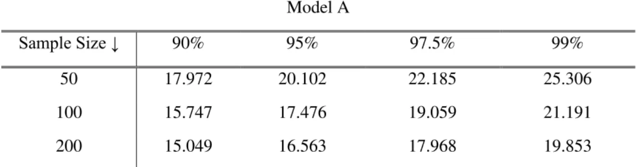
Table III: Selected percentiles of the distribution of _{𝑠𝑢𝑝𝜆∈𝛬𝐹𝝆̂}𝑖_(𝜆) Model A

Sample Size ↓ 90% 95% 97.5% 99%

50 17.972 20.102 22.185 25.306

100 15.747 17.476 19.059 21.191

21

>500 14.712 15.943 17.122 18.408

Model B

Sample Size ↓ 90% 95% 97.5% 99%

50 19.052 21.764 24.073 26.377

100 16.032 17.719 19.554 21.596

200 14.953 16.645 17.817 19.117

>500 14.019 15.367 16.622 18.183

Model C

Sample Size ↓ 90% 95% 97.5% 99%

50 21.950 24.388 26.556 30.175

100 18.712 20.585 22.253 24.619

200 17.601 18.691 20.339 22.383

>500 16.761 18.049 19.299 20.861

Testing for the null hypothesis goes as follows: Choose the Model (A, B or C)

that best describe the data from ₍₉₎, and estimate it by OLS for break fractions, _𝜆, going

from _{𝑗 = 2 𝑇}⁄ until _{𝑗 = (𝑇 − 1) 𝑇}⁄ . For each possible break fraction, it might be needed

to augment the test regression with lagged second differences of _𝑦𝑡 to remove the effect

of autocorrelated errors on the properties of the test statistics. The number 𝑘 of lags can

be determined with the GTS (General-to-Specific) methodology with the usual p-value

of 10% starting from _{𝑘 = 𝑘𝑚𝑎𝑥}. Then compute _𝐹𝝆̂𝑖_(𝜆) for each _𝜆, and choose the

greatest entry of the sequence of test statistics, and compare it with the respective

critical value presented in Table III. Reject the null hypothesis if the value of the test

22

6.3 Rejecting the Null Hypothesis

One key issue when testing for two unit roots is how to proceed when the test

leads to the rejection of the null hypothesis. In this case, the series can either be I(0) or

have a unit root. Several tests have been devised to test the null of exactly one unit root

when there is a break in the deterministic trend, such as Perron (1989), Zivot &

Andrews (1992) and more recently Perron (1997). Therefore, when rejecting the null

hypothesis of two unit roots, one natural suggestion is to proceed sequentially and in a

second step apply one of these tests for one unit root and conclude whether the series is

I(0) or I(1). Caution should be taken when a second test is performed sequentially,

because the overall test size increases with the application of a new individual test. The

difference between the significance level defined for each individual test and the

probability of Type I error of the sequential procedure is lwft for future research.

7 Size and Power Simulations

We now assess the finite sample power and size of the proposed tests. The data

generating processes for the Monte Carlo simulations are given by equations _{(3) 𝑖 =}

𝐴, 𝐵, 𝐶 and (5) with _{𝑒𝑡~𝑖. 𝑖. 𝑑 𝑁(0,1)}. The number of replications is set to 2500, and the

sample size is 50, 100, 200, 300, 400 and 500. The nominal size was fixed at _5% and

the asymptotic critical values from Table II were used for the test with a known break

date. The reported results are for Model A only, but Monte Carlo simulations for

Models B and C undertaken by the author of this thesis1 _{show identical outcomes. For}

the test with unknown break date the critical values from the Model A entry in Table III

were used. Because the null hypothesis assumes that no change occurs in the

deterministic function, we also investigate the robustness of the test to structural

23

changes under the null. In those simulations, the sample size is fixed in T=150 and _{𝜆 =}

1

2, while varying the break magnitude. Lastly, we inspect the behaviour of the test for an

unknown changepoint when multiple breaks occur, both under the null, and under

different alternatives, for Models A and B. In this case the sample size is also T=150.

Table IV: Null Rejection Probabilities – Known Changepoint Test

𝛼1, 𝛼2 ↓ 50 100 200 300 400 500

1.0, 1.0 0.046 0.018 0.021 0.034 0.033 0.041

1.0, 0.9 0.112 0.067 0.128 0.305 0.577 0.818

1.0, 0.7 0.287 0.249 0.434 0.782 0.960 0.998

0.9, 0.9 0.188 0.199 0.567 0.922 0.995 1.000

0.9, 0.8 0.315 0.427 0.861 0.966 0.999 1.000

0.99, 0.99 0.066 0.033 0.040 0.055 0.082 0.108

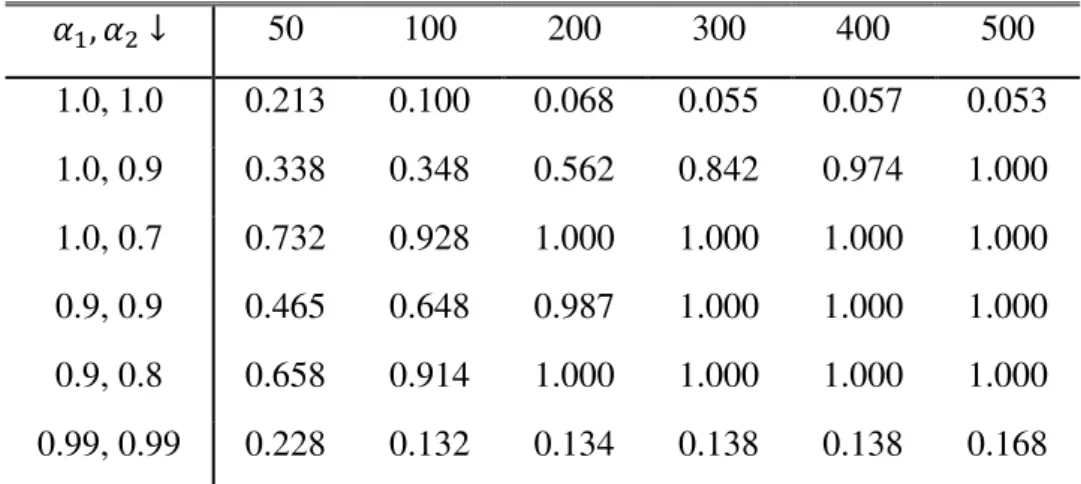
Table V: Null Rejection Probabilities – Unknown Changepoint Test

𝛼1, 𝛼2 ↓ 50 100 200 300 400 500

1.0, 1.0 0.213 0.100 0.068 0.055 0.057 0.053

1.0, 0.9 0.338 0.348 0.562 0.842 0.974 1.000

1.0, 0.7 0.732 0.928 1.000 1.000 1.000 1.000

0.9, 0.9 0.465 0.648 0.987 1.000 1.000 1.000

0.9, 0.8 0.658 0.914 1.000 1.000 1.000 1.000

0.99, 0.99 0.228 0.132 0.134 0.138 0.138 0.168

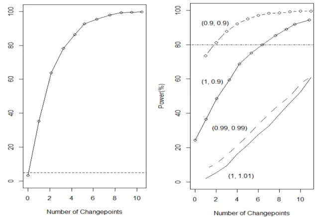
Starting with the test for a known breakpoint (Table IV), the empirical size is

very close to nominal 5%, even when the sample includes only 50 observations. When

the sample grows larger, the simulated size draws a U-shaped trajectory, with a

minimum close to 2% when the sample size is around 100 observations. However, it

24

The test also displays decent power to reject the null in finite samples against

several configurations of the alternative hypothesis. In the somewhat extreme case of

both roots equal to 0.99, the test presents very low power, close to the nominal size.

However, even in this case, we notice that power tends to increase with the sample size,

albeit at a very slow rate.

For the test with an unknown changepoint (Table V), there is a modest size

distortion in small samples. The test has finite sample power to reject the null, and lacks

power only in the extreme cases of both inverse roots equal to 0.99, although in the

25

Figure 2 - Size as a function of the break parameters. Model A (left) and Model B (right)

26

Figures 2-4 show the behaviour of the test for an unknown break date, under

different configurations. Figure 2 shows that a level shift (Model A) under the null

hypothesis leads to an oversized test, which is aggravated when the break parameter

grows larger. However, from Theorem 3, this problem disappears when the sample size

grows large. If instead of a level shift, we have a slope change (Model B) the effect is

almost negligible. The test becomes oversized, but the size distortion increases very

slowly with the magnitude of the break. Again, Theorem 3 ensures that this problem

does not exist in large samples.

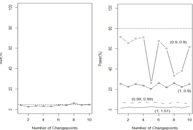
Figure 3 shows a similar exercise; however, this time it is the number of

breakpoints that changes. Here, both size and power increase with the number of breaks.

27

Figure 4 shows the effect of multiple changepoints, but for Model B. Here, the test size

and power remain almost unchanged.

8 Empirical Applications

We now apply the previous tests to a dataset composed of monthly, quarterly

and annual series. Information about the complete dataset can be found in the Data

Appendix. One relevant aspect to the application of the proposed tests is the choice of _𝑘,

i.e., the number of lagged second-differences, _Δ2_{𝑦𝑡−𝑖, 𝑖 = 1, … , 𝑘}, to be added in

equation _{(7. 𝑖)}. We opted to use a conventional GTS strategy with p-value=0.1, starting

from _{𝑘 = 𝑘𝑚𝑎𝑥}. The _{𝑘𝑚𝑎𝑥} chosen depended on the frequency of each time series. For

the annual series we used _{𝑘𝑚𝑎𝑥 = 4} or ₆, for the quarterly series we used _{𝑘𝑚𝑎𝑥 = 8} and

for the monthly series we used _{𝑘𝑚𝑎𝑥 = 24}. For each model, the sequence of test

statistics was calculated. Once the sequence of test statistics is obtained, we use the

estimate of the break date of each model, which is the one that corresponds to the

sup𝜆∈Λ𝐹𝝆̂𝑖(𝜆0), for 𝑖 = 𝐴, 𝐵, 𝐶, and rerun the test regression with those estimated break

dates and calculate the AIC and BIC information criteria. The chosen model is that

which minimizes these criteria. In the case of different models chosen, the Schwartz

criteria is favoured because it tends to choose a more parsimonious model. The results

are given in Table VI.

The test under the unknown changepoint framework was applied for all series,

except the Greek government debt. For the Greek Government Debt series, the test for a

known break date was used, since there is a clear level shift in the last quarter of 2013.

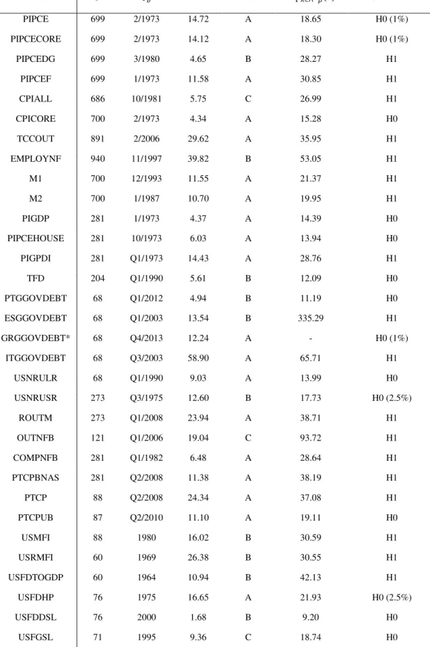
For the monthly series, the null hypothesis was rejected for all but three series when

28

test has excessive size-distortions when a level shift truly exists, even if the null

hypothesis is true. Structural changes are a common feature of long span data, thus, it is

possible that the null hypothesis is rejected due to the presence of a level shift. This

problem, and an eventual solution, will be discussed shortly.

For the quarterly series, we highlight the fact that for the Portuguese and Greek

General Government debts, the null hypothesis was not rejected meaning that

innovations have a very persistent behaviour. In fact, if we assume that the data can be

described by an _{𝐴𝑅𝐼𝑀𝐴(𝑝, 2, 𝑞)} process, then it is easy to understand and justify the

marked increase in debt observed in the latest years (several positive shocks), and why

it has been difficult to lower said debt (past shocks have its effects increased over time).

For the annual time series, there are some differences in both tests, namely for

some population series, which is an interesting outcome. For six population series, the

HF test rejects the null hypothesis, whilst the supremum test does not. Non-rejection of

the null hypothesis for the population series suggests that, with the right policies

(positive shocks), it might be possible to reverse the downward trend verified in many

developed countries. For Portugal, however, the null hypothesis was rejected when

using _{sup𝜆∈Λ𝐹𝝆̂}𝐴_(𝜆), but not rejected when using the common HF test, which seems to

go against the findings in Table I. However, note that the _{sup𝜆∈Λ𝐹𝝆̂}𝐴_(𝜆) might be

rejecting because there really is a level shift in 1974, which coincides with a major

29

Table VI: Tests for the Double Unit Root Null Hypothesis

Variable _{𝑇 𝑇𝑏}̂ HF test Model sup𝜆∈Λ𝐹𝜌̂𝑖(𝜆) Conclusion PIPCE 699 2/1973 14.72 A 18.65 H0 (1%)

PIPCECORE 699 2/1973 14.12 A 18.30 H0 (1%)

PIPCEDG 699 3/1980 4.65 B 28.27 H1

PIPCEF 699 1/1973 11.58 A 30.85 H1

CPIALL 686 10/1981 5.75 C 26.99 H1

CPICORE 700 2/1973 4.34 A 15.28 H0

TCCOUT 891 2/2006 29.62 A 35.95 H1

EMPLOYNF 940 11/1997 39.82 B 53.05 H1

M1 700 12/1993 11.55 A 21.37 H1

M2 700 1/1987 10.70 A 19.95 H1

PIGDP 281 1/1973 4.37 A 14.39 H0

PIPCEHOUSE 281 10/1973 6.03 A 13.94 H0

PIGPDI 281 Q1/1973 14.43 A 28.76 H1

TFD 204 Q1/1990 5.61 B 12.09 H0

PTGGOVDEBT 68 Q1/2012 4.94 B 11.19 H0

ESGGOVDEBT 68 Q1/2003 13.54 B 335.29 H1

GRGGOVDEBT* 68 Q4/2013 12.24 A - H0 (1%)

ITGGOVDEBT 68 Q3/2003 58.90 A 65.71 H1

USNRULR 68 Q1/1990 9.03 A 13.99 H0

USNRUSR 273 Q3/1975 12.60 B 17.73 H0 (2.5%)

ROUTM 273 Q1/2008 23.94 A 38.71 H1

OUTNFB 121 Q1/2006 19.04 C 93.72 H1

COMPNFB 281 Q1/1982 6.48 A 28.64 H1

PTCPBNAS 281 Q2/2008 11.38 A 38.19 H1

PTCP 88 Q2/2008 24.34 A 37.08 H1

PTCPUB 87 Q2/2010 11.10 A 19.11 H0

USMFI 88 1980 16.02 B 30.59 H1

USRMFI 60 1969 26.38 B 30.55 H1

USFDTOGDP 60 1964 10.94 B 42.13 H1

USFDHP 76 1975 16.65 A 21.93 H0 (2.5%)

USFDDSL 76 2000 1.68 B 9.20 H0

30

BEL 71 1998 7.11 B 16.19 H0

CAN 56 1998 14.09 A 18.25 H0

CHN 56 1996 10.22 B 60.99 H1

EMU 56 1974 10.44 B 17.42 H0

EUU 56 1976 11.01 B 16.88 H0

FIN 56 1999 17.46 A 37.23 H1

FRA 56 1973 11.43 B 17.15 H0

ITA 56 1989 3.47 B 21.12 H0

PRT 56 1974 9.14 A 39.17 H1

ESP 56 1993 11.54 A 15.64 H0

DE 56 1989 13.60 A 25.40 H0 (1%)

US 86 1947 3.72 C 26.44 H0 (2.5%)

One of the limitations of the proposed test for an unknown changepoint is that it

tends to reject the null hypothesis more often than it should, when a change in the

deterministic function exists. If the data series studied is not too long, then it is plausible

that, should it be present, a very reduced number of changepoints exist. With this in

mind, for those series in Table VI for which the null was rejected, the sample was split

in two using the estimated break date. Then, the test for two-unit roots was applied to

the longest segment. Table VII shows the results. The green entries indicate those series

for which the conclusion of the test changed, yellow indicate those for which the

conclusion did not change, and the grey series were not re-tested since the null had been

not rejected before. The letters in brackets, (L) and (R), indicate whether the left or right

subsample was used.

Having repeated the test, it was possible to reverse the conclusion in seven

series. However, splitting the samples in two led to small subsamples in five of those

31

Nonetheless, there are some interesting non-rejections of the null, such as the Spanish

debt, the US Debt to GDP ratio, and the Portuguese population suggesting that, for the

subsample considered, innovations have a very persistent impact, which can be well

described by the two-unit root model.

Table VII: Tests for the Double Unit Root Null Hypothesis - Revised

Variable 𝑇 𝑇̂𝑏 HF test Model sup𝜆∈Λ𝐹𝜌̂𝑖(𝜆) Conclude PIPCE 419 2/1973 14.72 A 18.65 H0 (1%)

PIPCECORE 419 2/1973 14.12 A 18.30 H0 (1%)

PIPCEDG 363 (R) 8/1980 14.74 B 20.24 H1

PIPCEF 372 (R) 9/1980 16.38 B 23.84 H1

CPIALL 298 (R) 8/2008 24.51 A 30.79 H1

CPICORE 420 2/1973 4.34 A 15.28 H0

TCCOUT 410 (L) 5/1950 23.36 B 29.23 H1

EMPLOYNF 490 (R) 11/1964 41.65 A 46.11 H1

M1 197 (R) 9/2008 8.14 A 16.83 H0

M2 255 (R) 5/1995 9.25 A 39.17 H1

PIGDP 169 1/1973 4.37 A 14.39 H0

PIPCEHOUSE 169 10/1973 6.03 A 13.94 H0

PIGPDI 123 (R) Q1/1981 15.81 B 25.24 H1

TFD 122 Q1/1990 5.61 B 12.09 H0

PTGGOVDEBT 41 Q1/2012 4.94 B 11.19 H0

ESGGOVDEBT 68 Q1/2003 13.54 B 335.29 H1

GRGGOVDEBT* 68 Q4/2013 12.24 A - H0 (1%)

ITGGOVDEBT 32 (R) Q1/2007 18.66 A 54.28 H1

USNRULR 164 Q1/1990 9.03 A 13.99 H0

USNRUSR 164 Q3/1975 12.60 B 17.73 H0 (2.5%)

ROUTM 60 (R) Q2/2000 14.05 A 25.13 H0 (1%)

OUTNFB 166 (L) Q1/1961 23.54 C 87.27 H1

COMPNFB 99 (L) Q2/1965 12.08 B 24.39 H1

PTCPBNAS 38 (R) Q3/1999 38.18 C 79.33 H1

PTCP 38 (R) Q1/2000 45.66 B 62.55 H1

32

USMFI 25 (R) 2000 12.66 B 21.55 H0

USRMFI 32 (R) 2000 20.23 B 24.25 H0 (1%)

USFDTOGDP 35 (R) 2008 11.75 A 14.83 H0

USFDHP 46 1975 16.65 A 21.93 H0 (2.5%)

USFDDSL 43 2000 1.68 B 9.20 H0

USFGSL 43 1995 9.36 C 18.74 H0

BEL 56 1998 7.11 B 16.19 H0

CAN 56 1998 14.09 A 18.25 H0

CHN 34 (R) 1974 13.99 B 61.26 H1

EMU 56 1974 10.44 B 17.42 H0

EUU 56 1976 11.01 B 16.88 H0

FIN 36 (R) 1969 14.01 A 61.20 H1

FRA 56 1973 11.43 B 17.15 H0

ITA 56 1989 3.47 B 21.12 H0

PRT 36 (R) 2006 6.29 C 20.60 H0

ESP 56 1993 11.54 A 15.64 H0

DE 56 1989 13.60 A 25.40 H0 (1%)

33

9 Conclusions

Structural changes affect the limiting distribution of the OLS estimator, and can

distort the inference based on non-robust methods. In this dissertation, we extended the

test proposed in Hasza & Fuller (1979) for two-unit roots, to cover the case of a possible

change in the deterministic function.

Two different approaches were developed, one that exploits information

available about the break date, and other that assumes no prior knowledge about it.

Under the known break date hypothesis, the test regression from the common

Hasza-Fuller test was adapted to include the information available. The test statistic has a

non-standard limiting distribution under the null hypothesis, which does not depend on

nuisance parameters, and its critical values are obtained via Monte Carlo simulation.

For the case of an unknown break date, a supremum approach was taken in order to

pinpoint the date that gives the highest evidence for the alternative hypothesis. The test

statistic has a non-standard limiting distribution, and is also free of nuisance parameters

under the null hypothesis. However, due to the way the null hypothesis is formulated,

the small sample distribution is perturbed by the break parameters. Nonetheless, this is

only a problem under model A with integrated errors, and it quickly dissipates as the

sample size grows large.

The tests were subject to a series of simulations in order to verify its robustness

against several alternatives. Both tests are asymptotically consistent and have the correct

size. One of the limitations of the test for an unknown break date is the excessive size

distortions, in small samples, when facing a level shift under the null hypothesis.

However, this problem vanishes asymptotically. This issue does not arise when there is

34

changepoint but, again only for model A and it vanishes with the increase of the sample

size.

In section 8, both tests were applied to several time series which are suitable

candidates to be explained by the two-unit root model. The null hypothesis was not

rejected for 23 of those time series, with special attention to the Portuguese and Greek

General Government debts. Other interesting results concern the natural rates of

unemployment for the United States and for many of the population series. It seems that

the double-unit root model is a suitable candidate to explain some major economic

variables.

The tests proposed are F type of statistics, and thus, bilateral in nature. This

means that additional power gains can be achieved by exploring unilateral t-tests, by

following for example the Dickey & Pantula approach. However, their method is more

complex since it requires changing the test regression in each step. Another issue that

should be solved in the unknown changepoint test starts by admitting a trend break

model even under the null hypothesis, to prevent excessive size distortions when there

is a level shift and the error is integrated of order two. Finally, it would be interesting to

35

References

Carrion-i-Silvestre, J. L., Kim, D., & Perron, P. (2009). GLS-based unit root tests with

multiple structural breaks under both the null and the alternative

hypotheses. Econometric Theory, 25(6), 1754-1792.

Cavaliere, G., Harvey, D. I., Leybourne, S. J., & Taylor, A. R. (2011). Testing for unit

roots in the presence of a possible break in trend and nonstationary

volatility. Econometric Theory, 27(5), 957-991.

Dickey, D. A., & Pantula, S. G. (1987). Determining the order of differencing in

autoregressive processes. Journal of Business & Economic Statistics, 5(4), 455-461.

Haldrup, N. (1994). Semi-parametric Tests for Double Unit Roots. Journal of Business

& Economic Statistics, 12, 109–122

Haldrup, N. (1998). A Review of the Econometric Analysis of I(2) Variables. Journal of

Economic Surveys, 12, 595– 650.

Hamilton, J. D. (1994). Time series analysis (Vol. 2). Princeton: Princeton university

press.

Harvey, D. I., Leybourne, S. J., & Taylor, A. R. (2009). Simple, robust, and powerful

tests of the breaking trend hypothesis. Econometric Theory, 25(4), 995-1029.

Harvey, D. I., Leybourne, S. J., & Taylor, A. R. (2013). Testing for unit roots in the

possible presence of multiple trend breaks using minimum Dickey–Fuller

statistics. Journal of Econometrics, 177(2), 265-284.

Hasza, D. P., & Fuller, W. A. (1979). Estimation for autoregressive processes with unit

36

Kim, D., & Perron, P. (2009). Unit root tests allowing for a break in the trend function

at an unknown time under both the null and alternative hypotheses. Journal of

Econometrics, 148(1), 1-13.

Lumsdaine, R. L., & Papell, D. H. (1997). Multiple trend breaks and the unit-root

hypothesis. The review of economics and statistics, 79(2), 212-218.

Montañés, A. (1997). Level shifts, unit roots and misspecification of the breaking date.

Economics Letters, 54(1), 7-13.

Nelson, C. R., & Plosser, C. R. (1982). Trends and random walks in macroeconmic time

series: some evidence and implications. Journal of Monetary Economics, 10(2),

139-162.

Patterson, K. (2011). Unit root tests in time series volume 1: key concepts and

problems. Springer.

Perron, P. (1989). The Great Crash, the oil price shock, and the unit root hypothesis.

Econometrica: Journal of the Econometric Society, 1361-1401.

Perron, P. (1997). Further evidence on breaking trend functions in macroeconomic

variables. Journal of econometrics, 80(2), 355-385.

Rodrigues, P. M., & Taylor, A. R. (2003). On Tests for Double Differencing: Some

Extensions and the Role of Initial Values. Documento de trabajo, 23.

Sen, D. L., & Dickey, D. A. (1987). Symmetric test for second differencing in

univariate time series. Journal of Business & Economic Statistics, 5(4), 463-473.

Shin, D.W. and Kim, H.J. (1999). Semiparametric Tests for Double Unit Roots Based

37

Zivot, E., & Andrews, D. W. K. (1992). Further evidence on the great crash, the

oil-price shock, and the unit-root hypothesis. Journal of Business & Economic Statistics,

38

A Data Appendix

Table VIII: Dataset Description

Variable Description Freq. Nº Obs.

PIPCE USA - Personal Consumption Expenditure Price Index (2009=100) M 699

PIPCECORE USA - Personal Consumption Expenditure Price Index, less Food and Energy (2009=100)

M 699

PIPCEDG USA - Personal Consumption Expenditure Price Index, Durable Goods (2009=100)

M 699

PIPCEF USA - Personal Consumption Expenditure, Food (2009=100) M 699

CPIALL USA - Consumer Price Index, All Items (2010=100) M 686

CPICORE USA - Consumer Price Index, less Food and Energy (2010=100) M 686

TCCOUT USA - Total Consumer Credit Owned and Securitized, Outstanding Bn. $ M 891

EMPLOYNF USA - Total Employment, Non-Farm M 940

M1 USA - M1 Money Stock M 700

M2 USA - M2 Money Stock M 700

PIGDP USA - Gross Domestic Product Price Index (2009=100) Q 281

PIPCEHOUSE USA - Personal Consumption Expenditure Price Index – Housing (2009=100)

Q 281

PIGPDI USA - Gross Private Domestic Investment Price Index (2009=100) Q 281

TFD USA - Total Federal Debt, Million $ (no sa) Q 204

PTGGOVDEBT Portuguese General Government Debt, Million € Q 68

ESGGOVDEBT Spanish General Government Debt, Million € Q 68

GRGGOVDEBT Greek General Government Debt, Million € Q 68

ITGGOVDEBT Italian General Government Debt, Million € Q 68

USNRULR USA – Natural Rate of Unemployment, Long Run Q 68

USNRUSR USA – Natural Rate of Unemployment, Short Run Q 68

ROUTM USA - Real Output - Manufacturing Q 121

OUTNFB USA – Non Farm Business Sector – Real Output Q 281

COMPNFB USA – Non Farm Business Sector – Compensation per Hour Q 281

PTCPBNAS PT – Private Consumption. Services and non Food Goods Q 88

PTCP PT – Private Consumption Q 88

PTCPUB PT – Public Consumption Q 88

USMFI Mean Family Income – USA A 63