DM
TD
October | 2016
Hardware and Software Platforms
to Deploy and Evaluate Non-Intrusive
Load Monitoring Systems
DOCTORAL THESIS
Amâncio Lucas de Sousa Pereira
Load Monitoring Systems
DOCTORAL THESIS
Amâncio Lucas de Sousa Pereira
DOCTORATE IN INFORMATICS ENGINEERING SPECIALTY: SOFTWARE ENGINEERING
SUPERVISOR
Duarte Nuno Jardim Nunes
CO-SUPERVISOR
I hereby declare that except where specific reference is made to the work of others, the
contents of this dissertation are original and have not been submitted in whole or in part for
consideration for any other degree or qualification in this, or any other University. This
dissertation is the result of my own work and includes nothing, which is the outcome of work
done in collaboration, except where specifically indicated in the text. This dissertation
contains less than 200 pages, excluding indices, bibliography and appendixes.
Lucas Pereira
The work in this PhD thesis addresses the practical implications of deploying and testing
Non-Intrusive Load Monitoring (NILM) and eco-feedback solutions in real-world scenarios.
The contributions to this topic are centered around the design and development of NILM
frameworks that have been deployed in the wild, supporting long-term research in
eco-feedback and also serving the purpose of producing real-world datasets and furthering the
state of the art regarding the performance metrics used to evaluate NILM algorithms.
This thesis consists of three main parts: i) the development of tools and datasets for
NILM and eco-feedback research, ii) the design, implementation and deployment of NILM
and eco-feedback technologies in real world scenarios, and iii) an experimental comparison
of performance metrics for event detection and event classification algorithms.
In the first part we describe the Energy Monitoring and Disaggregation Data Format
(EMD-DF) and the SustData and SustDataED public datasets.
In second part we discuss the development and deployment of two hardware and software
platforms in real households, to support eco-feedback research. We then report on more than
five years of experience in deploying and maintaining such platforms. Our findings suggest
that the main practical issues can be divided in two categories, technological (e.g., system installation) and social (e.g., maintaining a steady sample throughout the whole study).
In the final part of this thesis we analyze experimentally the behavior of a number of
performance metrics for event detection and event classification, identifying clusters and
relationships between the different measures. Our results evidence some considerable
differences in the behavior of the performance metrics when applied to the different
problems.
Keywords: NILM, Event-Based, Eco-Feedback, Performance evaluation, Platforms, Real
O trabalho desenvolvido nesta tese de doutoramento aborda as implicações praticas da
instalação e avaliação de soluções de monitorização não intrusiva de cargas elétricas (NILM)
e eco-feedback em cenários reais. As contribuições para este tópico estão centradas em torno
da concepção e desenvolvimento de plataformas NILM que foram instaladas em ambientes
não controlados, suportando a pesquisa de longo termo em eco-feedback e servindo também
o propósito de produzir conjuntos de dados científicos, bem como promover o avanço do
estado da arte acerca das métricas de desempenho utilizadas para avaliar algoritmos NILM.
Esta tese é constituída por três partes principais: i) o desenvolvimento de ferramentas e
conjuntos de dados científicos para investigação em NILM e eco-feedback, ii) a concepção,
desenho e instalação de tecnologias NILM e eco-feedback em cenários reais, e iii) uma
comparação experimental de métricas de desempenho para algoritmos de detecção e de
classificação de eventos.
Na primeira parte descrevemos o Energy Monitoring and Disaggregation Data Format
(EMD-DF) e os conjuntos de dados científicos SustData e SustDataED.
Na segunda parte discutimos o desenvolvimento e instalação de duas plataformas de
hardware e software em residências atuais com a finalidade de suportar a investigação em
eco-feedback. Aqui, reportamos sobre mais de cinco anos de experiência na instalação e
manutenção destes sistemas. Os nossos resultados sugerem que as principais implicações
práticas podem ser divididas em duas categorias, físicas (e.g., instalação do sistema) e sociais
(e.g., manter uma amostra constante ao longo de todo o estudo).
Na terceira parte analisamos experimentalmente o comportamento de uma série de
métricas de desempenho quando estas são utilizadas para avaliar algoritmos de detecção e de
classificação de eventos. Calculamos as correlações lineares e não lineares entre os vários
Palavras-chave: NILM, Baseado-em-eventos, Eco-Feedback, Avaliação de performance,
Thesis Contents ... ix
List of Figures ... xi
List of Tables ... xv
Chapter 1 Introduction ... 1
1.1 Context ... 1
1.2 Motivation ... 4
1.3 Problem Statement ... 6
1.4 Thesis Outline ... 7
Chapter 2 Non-Intrusive Load Monitoring ... 9
2.1 Seminal Work ... 9
2.2 Event-Based and Event-Less Approaches ... 10
2.3 Existing Challenges ... 13
2.4 Literature Review on Load Disaggregation ... 15
2.5 Literature Review on Performance Evaluation ... 24
Chapter 3 Research Scope ... 41
3.1 Research Questions ... 41
3.2 Research Method ... 43
3.3 Research Contributions ... 45
3.4 Publications ... 48
Chapter 4 Tools and Datasets ... 53
4.1 EMD-DF: Energy Monitoring and Disaggregation Data Format ... 53
4.2 SustData: A Public Dataset for Electric Energy Research ... 71
4.3 SustDataED: A Public Dataset for Electric Energy Disaggregation Research ... 80
Chapter 5 NILM Deployments in Real World Scenarios ... 89
5.1 Introduction ... 90
5.2 Research Platform Overview ... 93
5.3 Practical Deployment Considerations ... 105
6.1 Algorithms ... 126
6.2 Datasets ... 143
6.3 Performance Metrics ... 146
6.4 Experimental Design ... 152
6.5 Analysis of Results ... 168
6.6 Conclusion ... 187
Chapter 7 Conclusion and Future Work ... 193
7.1 Chapter Summaries ... 193
7.2 Future Work ... 194
Bibliography ... 199
Appendix A Background Research ... A-1
A.1 A Survey of Smart-Meters ... A-1
A.2 A Survey of Public Household Energy Datasets ... A-13
Appendix B Research Datasets ... B-1
B.1 UK-DALE ... B-1
B.2 BLUED ... B-3
B.3 PLAID ... B-5
Appendix C Performance Metrics ... C-1
C.1 Event Detection ... C-1
C.2 Event Classification ... C-9
Appendix D Additional Tables ... D-1
D.1 Parameter and Feature Sweep Lookup Tables ... D-1
D.2 Performance Metrics Pairwise Correlations ... D-6
Appendix E Additional Resources ... E-1
Figure 1.1 – Total electricity consumption by end-use sector: 2010 (left), 2040 (right) ... 2
Figure 2.1 – Example of event-based energy disaggregation ... 12
Figure 2.2 – Example of event-less energy disaggregation ... 12
Figure 2.3 – General workflow for event-based NILM approaches ... 16
Figure 4.1 – EMD-DF: Data model overview ... 54
Figure 4.2 - RIFF chunk format definition ... 55
Figure 4.3 – RIFF-WAVE file format chunk structure ... 57
Figure 4.4 - Example of an Appliance Activity Annotation ... 62
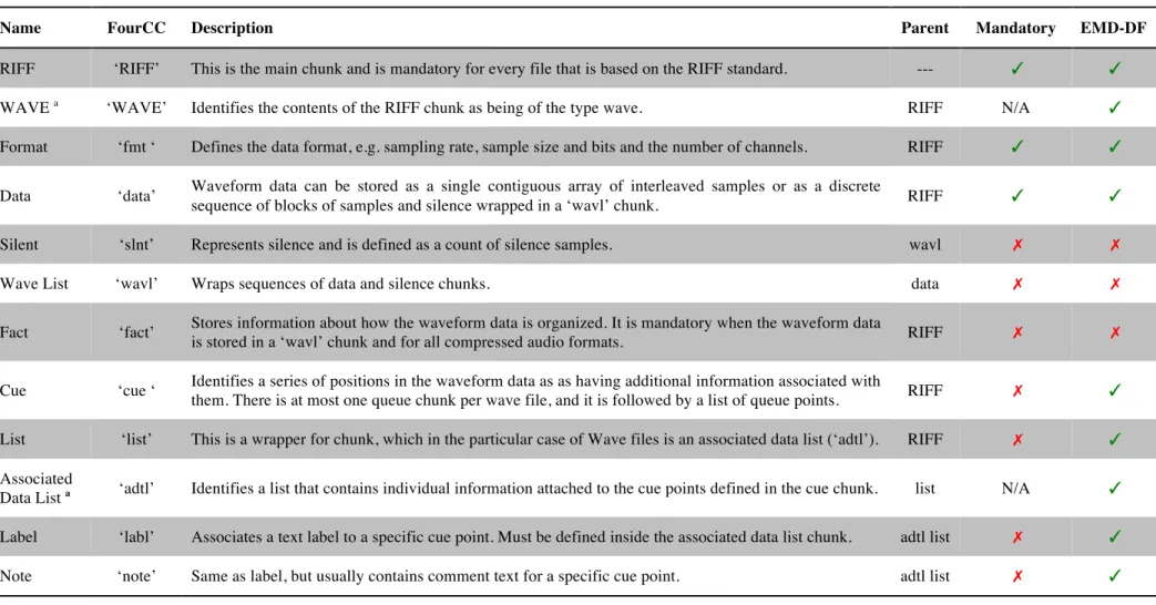
Figure 4.5 - Markers for the refrigerator events in the P & Q file at 60 Hz (top), and one marker at the I & V file at 12 kHz (bottom) ... 63
Figure 4.6 - Example of user activity annotation ... 64
Figure 4.7 - Example of a Local Metadata Annotation ... 65
Figure 4.8 – Appliances custom metadata annotation ... 66
Figure 4.9 - User activities custom metadata annotation ... 66
Figure 4.10 – NILM Metadata project custom chunk ... 67
Figure 4.11 – Real power transient of a microwave turning ON ... 76
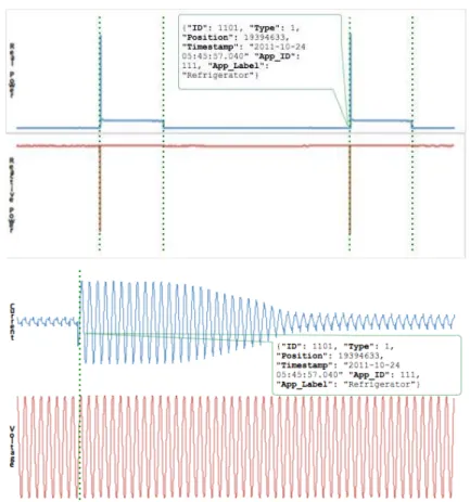
Figure 4.12 – Aggregate consumption vs. the sum of the individual appliances summarized by day and hour ... 86
Figure 4.13 – EMD-DF configuration information: raw voltage and current (left), processed waveforms (right) ... 87
Figure 5.1 - Energy monitoring and eco-feedback research platform overview ... 91
Figure 5.2 – Sensing hardware: split-core current sensor (left), voltage transformer (center) and TRS splitter connectors (right). ... 94
Figure 5.3 – Current and voltage sensors installed in the main power feed ... 95
Figure 5.4 – Energy eco-feedback is provided on-site using the netbooks’ built-in LCD screen ... 96
Figure 5.8 – Multi-house platform installation: current sensors (left), voltage sensors and DAQ (right) ... 99
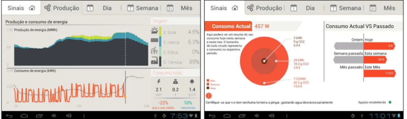
Figure 5.9 – Energy eco-feedback applications used in deployment two: energy awareness mode (left), detailed consumption mode (right) ... 100
Figure 5.10 - ... 101
Figure 5.11 – Example of a possible configuration of the multi-house energy monitoring platform ... 102
Figure 5.12 – Research platforms deployment timeline ... 103
Figure 5.13 – The energy monitors are attached to the main fuse door with sticky back Velcro straps ... 103
Figure 5.14 – Major milestones of deployment one (top); active installations over time
(bottom) ... 104
Figure 5.15 – Multi-port DAQs installed in the main electric panel of one of the buildings 104
Figure 5.16 – Major milestones of deployments two and three (top); active installations over time (bottom) ... 105
Figure 5.17 – MySQL vs. MongoDB: database physical size ... 108
Figure 5.18 – MySQL vs. MongoDB: average query time ... 109
Figure 5.19 – Single- vs. Multi-House: Hardware costs associated with monitoring one house ... 113
Figure 5.20 – Single- vs. Multi-House vs. Multiple Sensors: Hardware costs associated with monitoring one house ... 115
Figure 5.21 – Differences in hardware costs projected up to 5000 houses. ... 115
Figure 5.22 – Estimated energy costs of different energy monitoring solutions after one year ... 117
Figure 5.23 – Proportion of aggregate to power event data for one house after one year ... 119
Figure 6.1 – Illustration of the MEH event detection process. Real power and absolute power changes (top), threshold filter (center), elapsed time filter (bottom) ... 129
Figure 6.2 – Illustration of the LLD event detection process. Active power and detection statistic (top), voting procedure (center), and votes filtered by threshold (bottom) ... 133
Figure 6.3 – Illustration of the SLLD event detection process. Active power and detection statistics (top), detection statistics and local maxima (center), active power and power events (bottom) ... 136
Figure 6.4 – Flowchart of the algorithm used to create the contingency table of the event detection algorithms ... 163
Figure 6.5 – List of metric pairs with pairwise correlations above 0.9 in at least of one the coefficients ... 174
Figure 6.6 – Dendrograms showing ranks (left) and linear (right) correlations of the
Figure 6.8 – SLLDMax (BLUED – A): Precision and Recall based metrics sorted in ascending order of detected events (line series). Top 10 models selected by the each metric (column series). ... 177
Figure 6.9 – Dendrograms showing ranks (left) and linear (right) correlations of the micro-average performance metrics across datasets ... 183
Figure 6.10 – TOP 5 models selected by the micro-average and probabilistic metrics ... 184
Figure 6.11 – Dendrograms showing ranks (left) and linear (right) correlations of the
unweighted macro-average performance metrics across datasets ... 185
Figure 6.12 - Dendrograms showing ranks (left) and linear (right) correlations of the
weighted macro-average performance metrics across datasets ... 185
Figure 7.1 –Single sensor (Left) and Multiple sensor (Right) ... A-3
Figure 7.2 - The Energy Detective smart-meter solution: Packaged hardware (Left) and installation in the main breaker box (Right). ... A-4
Figure 7.3 - EnerSure branch circuit power meter: Metering unit (Left) and installation in the main breaker box (Right). ... A-5
Figure 7.4 - Multiple sensor smart-meters: Belkins Conserve (Left) and P3 Internationals Kill-a-Watt CO2 Wireless (Right ... A-8
Figure 7.5 – UK-DALE 1: Distribution of power events in terms of the absolute active power change; all events (left); events below 100 Watts (right) ... B-1
Figure 7.6 – UK-DALE 1: Boxplot showing the distribution of the power events according to the absolute power change. ... B-2
Figure 7.7 – UK-DALE 2: Distribution of power events in terms of the absolute active power change; all events (left); events below 100 Watts (right) ... B-2
Figure 7.8 – UK-DALE 2: Boxplot showing the distribution of the power events according to the absolute power change. ... B-3
Figure 7.9 – BLUED A: Distribution of power events in terms of the absolute active power change; all events (left); events below 100 Watts (right) ... B-3
Figure 7.10 – BLUED A: Boxplot showing the distribution of the power events according to the absolute power change. ... B-4
Figure 7.11 – BLUED B: Distribution of power events in terms of the absolute active power change; all events (left); events below 100 Watts (right) ... B-4
Figure 7.12 – BLUED 2: Boxplot showing the distribution of the power events according to the absolute power change. ... B-5
Figure 7.13 – PLAID: Appliance instances distribution in each dataset partition ... B-6
Table 2.1 – Appliance types definitions and examples ... 11
Table 2.2 – Overview of public household energy datasets ... 27
Table 2.3 – Performance metrics for NILM approaches. (EB: Event-Based; EL: Event-Less) ... 36
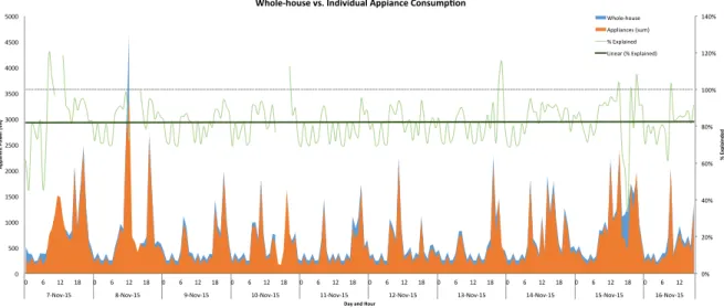
Table 4.1 – List of chunks that compose the RIFF-WAVE file format ... 58
Table 4.2 - List of chunks that compose EMD-DF ... 60
Table 4.3 - List of RIFF metadata chunks ... 67
Table 4.4 – List of functions available to create and maintain EMD-DF based datasets ... 68
Table 4.5 - Household demographic features ... 72
Table 4.6 – Summary of household demographics ... 72
Table 4.7 – Household member demographic features ... 73
Table 4.8 - Summary of household member demographics ... 73
Table 4.9 – Energy consumption measurements ... 74
Table 4.10 – Summary of the energy consumption data ... 75
Table 4.11 – Power event measurements ... 75
Table 4.12 - Power events summary ... 76
Table 4.13 – User event features ... 77
Table 4.14 – Summary of user events ... 77
Table 4.15 - Environmental data measurements ... 78
Table 4.16 - Electric energy production measurements ... 78
Table 4.17 – Summary of the individual appliance and occupancy data that can be found in SustDataED ... 84
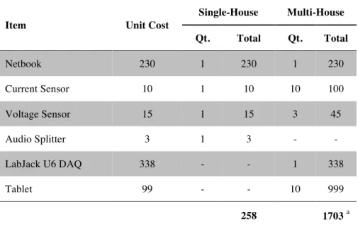
Table 5.1 – Baseline hardware costs of the single- and multi-house energy monitors ... 112
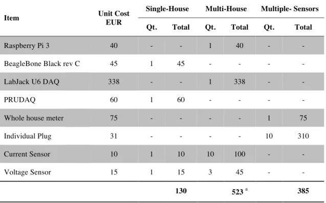
Table 5.2 - Baseline hardware costs of the single- and multi-house energy monitors ... 114
Table 5.3 – Estimated energy costs of the components that compose the monitoring solutions ... 116
Table 6.1 – Event detection algorithms to be evaluated ... 126
Table 6.2 – Parameter space of Meehan s et al. expert heuristic event detector ... 128
Table 6.3 – Parameter space for the Log Likelihood Ratio event detector ... 131
Table 6.4 – Parameter space of the voting algorithm used in the LLR event detector ... 132
Table 6.5 – Parameter space of the maxima algorithm used in the SLLR detector ... 135
Table 6.6 – Selected classification algorithms ... 137
Table 6.7 – Summary of the datasets used to evaluate detection algorithms ... 144
Table 6.8 - Summary of the active power change and elapsed time between power events in the event detection datasets ... 145
Table 6.9 – Datasets used for event classification ... 145
Table 6.10 - Summary of performance metrics for event detection ... 147
Table 6.11 – Summary of rank metrics for event detection algorithms ... 148
Table 6.12 – Summary of domain specific metrics for event detection algorithms ... 149
Table 6.13 – Confusion matrix based metrics for event classification ... 150
Table 6.14 – Summary of rank metrics for event classification ... 151
Table 6.15 – Summary of probabilistic metrics for event classification ... 152
Table 6.16 – List of possible pairwise correlations per metric types ... 154
Table 6.17 – Parameter ranges for Meehan Expert Heuristic event detector ... 157
Table 6.18 – Parameter ranges for Log-Likelihood and Simplified Log-Likelihood detectors with votingactivation. ... 158
Table 6.19 – Parameter ranges for Log-Likelihood and Simplified Log-Likelihood detectors with maximaactivation. ... 159
Table 6.20 – Number of different models that will be evaluated across datasets ... 160
Table 6.21 – Tolerance values for event detection evaluation ... 161
Table 6.22 – List of the parameters that will be switched in each classification algorithm and respective values ... 164
Table 6.23 – Different feature sets used in the event classification algorithms ... 167
Table 6.24 – Rank (bottom-left) and linear (top-right) correlation results for all four datasets ... 170
Table 6.25 – Rank and linear correlations averaged by metric for the four event detection datasets ... 171
Table 6.26 – Clusters formed after cutting the dendrograms of the cross dataset non-linear and linear correlations ... 175
Table 6.27 – Micro average metrics: rank (bottom-left) and linear (top-right) correlation results for all datasets ... 179
Table 6.30 – Rank and linear correlations averaged by metric for all datasets ... 182
Table 6.31 – Unweighted macro-average clusters ... 186
Table 6.32 – Weighted macro-average clusters ... 186
Table 7.1 – Shortlist of single sensor smart-meter alternatives ... A-6
Table 7.2 – Shortlist of multiple sensor smart-meter alternatives ... A-11
Table 7.3 – PLAID: Appliance instances distribution in each dataset partition ... B-5
Table 7.4 – Different parameter configurations for the MEH algorithm (50 Hz and 60 Hz datasets) ... D-2
Table 7.5 – Different parameter combinations for the LLD algorithm (50 Hz datasets) ... D-3
Table 7.6 – Different parameter combinations for the LLD algorithm (60 Hz datasets) ... D-4
Table 7.7 – Different parameter configurations for the SLLD algorithm (50 Hz and 60 Hz datasets) ... D-5
Table 7.8 – Different parameter and feature configurations for the six event classification algorithms ... D-5
Table 7.9 – Different parameters and possible values for each of the six classification
algorithms ... D-6
Table 7.10 – Different feature combinations for the six classification algorithms ... D-6
Table 7.11 – MEH event detector: cross dataset pairwise correlations ... D-7
Table 7.12 – SLLDMax event detector: cross dataset pairwise correlations ... D-7
Table 7.13 – LLDMax event detector: cross dataset pairwise correlations ... D-8
Table 7.14 – SLLDVote event detector: cross dataset pairwise correlations ... D-8
Table 7.15 – LLDVote event detector: cross dataset pairwise correlations ... D-9
Table 7.16 – K-NN classifier: cross dataset pairwise correlations for micro-average metrics D-9
Table 7.17 – KStar classifier: cross dataset pairwise correlations for micro-average metrics D-10
Table 7.18 – LWL with Naïve Bayes classifier: cross dataset pairwise correlations for micro-average metrics ... D-10
Table 7.19 – Decision Trees classifier: cross dataset pairwise correlations for micro-average metrics ... D-11
Table 7.20 – ANN classifier: cross dataset pairwise correlations for micro-average metrics . D-11
Table 7.21 – SVM classifier: cross dataset pairwise correlations for micro-average metrics . D-12
Table 7.22 – K-NN classifier: cross dataset pairwise correlations for unweighted macro-average metrics ... D-12
Table 7.25 – Decision Trees classifier: cross dataset pairwise correlations for unweighted macro-average metrics ... D-14
Table 7.26 – ANN classifier: cross dataset pairwise correlations for unweighted
macro-average metrics ... D-14
Table 7.27 – SVM classifier: cross dataset pairwise correlations for unweighted
macro-average metrics ... D-15
Table 7.28 – K-NN classifier: cross dataset pairwise correlations for weighted macro-average metrics ... D-15
Table 7.29 – KStar classifier: cross dataset pairwise correlations for weighted macro-average metrics ... D-16
Table 7.30 – LWL with Naïve Bayes classifier: cross dataset pairwise correlations for
weighted macro-average metrics ... D-16
Table 7.31 – Decision Tree classifier: cross dataset pairwise correlations for weighted macro-average metrics ... D-17
Table 7.32 – ANN classifier: cross dataset pairwise correlations for weighted macro-average metrics ... D-17
Table 7.33 – SVM classifier: cross dataset pairwise correlations for weighted macro-average metrics ... D-18
1.1
Context
The global demand for energy has been steadily increasing since 1990 and it is set to grow by
37% between 2012 and 2040 (from 13157 Mtoe in 2012 to an estimated 18419 Mtoe in
2040), according to the International Energy Agency [1]. This growth is mostly driven by the
emerging economies in Asia (60% of the global total), Africa, Middle East and Latin
America, contrasting the most developed nations in Europe, North America and Pacific that
manage to maintain a near-steady demand during that period [1].
Likewise, electricity consumption has been experiencing a steady increase since 1990, in
large part led by the BRICS1
countries who shared among them 35% of the total world
electricity consumption in 2012. As a matter of fact, these numbers are only a reflection of
how the world evolved in the last couple of decades, with electricity emerging as the second
most used end form of energy with a 17.7% share, only behind oil with 40.8% [2].
One of the leading factors for this growth in electricity demand is the change in energy
consumption habits in domestic environments which was, in 2010, responsible for 28% of the
final electricity consumption among all sectors (Figure 1.1 – left), a figure which represents
an overall increase of almost 40% between 1990 and 2010 [3].
11
Figure 1.1 – Total electricity consumption by end-use sector: 2010 (left), 2040 (right)
One of the factors leading to the growth in electricity consumption in the last years is the
notion of wellbeing based on personal ownership and mass consumption. As more people in
developing countries have access to higher levels of comfort it is expected that the world’s
demand for electricity will continue to increase in the next couple of decades. In fact,
according to the U.S. Energy Information Administration [3], it is expected that the demand
for electricity in residential and commercial buildings will see an average annual percent
increase of 2.6% and 2.5%, respectively, until 2040 reaching, by then, 32% and 26% of the
final energy consumption (Figure 1.1 – right).
Nevertheless, improvements in the quality of life enabled by electricity (e.g., improved
heating and ventilation systems, more and better electrical appliances, etc.) do not come
without environmental costs. In fact, evidence shows that the carbon dioxide emissions from
fuel combustion used to generate electrical energy, have also been steadily increasing since
1990. An increase that is particularly evident in the emerging economies (BRICS), which
have shown an average yearly increase of 5.4% between 2000 and 2012.
Furthermore, with energy-related carbon dioxide emissions expected to grow 46% by
2040, it is expected that residential energy consumption will contribute significantly for the
degradation of our eco-systems. Hence, the importance of domestic electric energy in the
global context of energy overconsumption as outlined in [4] where the authors mention that
residential buildings hold the potential for achieving one of the seven stabilization wedges
In particular, green building techniques are expected do play an important role in
reducing the impact of space thermal comfort (HVAC2), lighting and water heating through
smart construction strategies (e.g., effective window placement, wall and roof insulation and
solar water heating). Whilst current technology already offers appliances that consume less
power while delivering the same or better results, e.g. LED devices (lights and TVs) and
energy-efficient appliances like refrigerators that are expected to use about 15% less energy
than the traditional ones3. Yet, even though substantial savings can be achieved through
technology that is currently available, most of these are still expensive or have payback times
that are too prolonged in time to make them appealing to the general population of domestic
consumers.
Moreover, research indicates that a scenario where infrastructures themselves require less
energy would raise the problem of perverse incentives4 that suggest that the cheaper
something is, the more it will be used [5]. This is supported by reports suggesting that the low
price of electricity in some regions is one of the reasons behind the increase of electrical
energy consumption. Therefore, despite the potential savings that can be achieved with these
technological solutions, it does not necessarily mean that this would result in lower energy
consumption and, consequently, reduced carbon dioxide emissions.
In fact, literature reveals that the real potential for reducing energy consumption lies with
the consumers making a more efficient use of the house utilities and not so much on the
buildings themselves. Many studies suggest that providing users with real-time and historical
information about their consumption can lead to potential savings between 5% and 10% [6],
[7], especially in the cases where the feedback is enhanced with individual appliance
consumption information [8].
This is commonly known as eco-feedback technology and is defined as the technology that provides feedback on individual or group behaviors with a goal of reducing environmental impact [9]. The basic assumption behind eco-feedback technology is that
2
HVAC is the acronym for Heating, Ventilations and Air Conditioning technology 3
Energy Start, www.energystar.gov 4
people will be able to change their actions and consequently reduce their consumption if they
are able to understand which appliances are responsible for their overall energy consumption
breakdown.
This was especially noticed in [7], where Parker and colleagues evaluated two low-cost
monitoring systems and found that users quickly discovered that by simply examining the
differences in the overall demand by turning appliances ON and OFF they could easily approximate the energy usage of each individual appliance.
As a consequence, there has been a substantial effort to create monitoring solutions that
are able to provide the consumption figures of individual appliances. Including, for instance,
electrical sub-metering (i.e., installing individual sensors in each appliance) or the
development of smart appliances that are able to communicate their own energy
consumption to a central gateway.
Yet, despite the fact that the reported results are mostly positive regarding improved
awareness and achieving savings in energy consumption [6], it has been also reported that
after an initial period of exposure to this technology the tendency is towards a decrease in the
attention given to the feedback leading to behavior relapse [10], [11]. This is defined in
literature as the response-relapse effect and suggests that in order to properly assess the effectiveness of eco-feedback as a tool for promoting sustained energy saving, future studies
should be carried for longer periods of time.
Furthermore, the intrinsically intrusive nature of such solutions implies that the
information about the consumption of individual appliances will be associated with higher
installation and maintenance costs that may obfuscate the potential savings [12].
1.2
Motivation
Against this background, there has been a significant research effort devoted to the
development of non-intrusive load monitoring (NILM) techniques that are able to sense and
in the electric distribution grid, hence contrasting the more traditional intrusive monitoring
technology that involve deploying multiple sensors throughout the house.
Early research in this topic dates back to 1985, when George Hart from the Massachusetts
Institute of Technology (MIT) coined the term Non-Intrusive (Appliance) Load Monitoring
(NIALM) [13] [14]. In very simple terms we define NILM as a set of signal-processing and machine-learning techniques that are used to estimate the aggregate and individual appliance electricity consumption from current and voltage measurements taken at a
limited number of locations in the electric distribution of a house (optimally the mains, hence covering the demand of the entire house).
Still, it was only in recent years that NILM gained renewed attentions from the research
community, in part due to the potential of such advanced metering technologies in promoting
overall year-round and indirect short-term energy saving strategies, which are expected to considerably reduce the carbon footprint associated with electric energy consumption.
Furthermore, NILM is expected to serve as the backbone technology that will enable the
creation of innovative smart-grid services that go beyond helping individuals saving energy,
as it was recently observed in the 2016 edition of the international NILM workshop [15].
The potential benefits of NILM include for example:
• The lower costs of installation and maintenance of NILM systems, enables the
deployment of long-term energy efficiency programs like eco-feedback, which are
necessary in order to access to long-term effectiveness of such programs.
• Having energy consumption disaggregated by appliance also enables the creation of
novel energy efficiency services. These include, the possibility of inferring and
providing eco-feedback on the everyday activities, e.g., preparing meals or taking care
of the laundry [16], [17].
• Additionally, NILM technology also enables the detection of anomalies in the electric loads [18], [19], which can result in the early detection of malfunctioning appliances,
This being said, it is not totally unexpected that recent times have seen a considerable
increase in the body of work in the field of energy disaggregation, which is naturally reflected
in the exponential grow of published papers in the topic [20] as well as in the recent boost in
the number of companies offering NILM products and services [21], [22].
Yet, and despite the growing body of work in this field, there are still many challenges
that must be solved before it is possible to take full advantage of the potential benefits of
low-cost and reliable NILM solutions. These are grouped according to two categories, namely: i)
load identification, and ii) training and supervision challenges [23].
As the name suggests, the former encompasses the different issues related to the problem
of correctly identifying the loads in the ever-growing complexity of the electric grid (e.g., different types of load and simultaneous load switching) and are naturally the focus of much
of the undergoing research [24], [25]. On the other hand, the latter encompasses the issues
related to the replication and generalization of research findings (e.g., the lack of proper test and training data and the inexistence of a formal agreement on how to report the
disaggregation results) and only recently have become the focus of a smaller group of NILM
researchers [26], [27].
Furthermore, and despite the abundance of literature, it was until only recently that we
saw the first publications regarding the value proposition of NILM as a tool to reduce energy
consumption, or trying to educate the research community about the practical issues of
deploying such systems in real world scenarios [28]–[31], which we believe are of crucial
importance to the large-scale adoption of NILM technology in years to come.
1.3
Problem Statement
As previously explained, despite the growing body of work in NILM research, there are still
some underexplored areas. This is particularly evident when it concerns to the practical issues
of deploying NILM systems or conducting formal evaluations and benchmarks of the
proposed algorithms, which are the main topics of the work in this thesis. To state more
Firstly, we will focus our attention on understanding the practical issues of deploying
NILM and eco-feedback systems in the domestic environments. These practical issues
include for instance, the ease of installation and use of the monitoring equipment, which may
ultimately affect how such systems are received and adopted by the residential sector.
Secondly, we will focus our attention on understanding the challenges of defining a
consistent set of performance metrics for the energy disaggregation problem. More
concretely, we propose to study the compatibility of existing performance metrics with the
nature and structure of the data generated by the different NILM algorithms, which may
ultimately change the way the different metric are used to draw conclusions regarding the
performance of such algorithms.
1.4
Thesis Outline
The remaining chapters of this thesis are organized as follows. In Chapter 2, we provide a
comprehensive background and literature review on NILM. Then, in Chapter 3 we formalize
the research questions addressed in this thesis and present the methods we will use to answer
these questions.
Following that, the main body of this thesis will be divided in three chapters. First, in
Chapter 4 we propose a data format to represent energy disaggregation datasets, and present
two public datasets that emerged from the work in this thesis. Then, in Chapter 5 we describe
two bespoke energy monitoring and eco-feedback platforms, and thoroughly discuss the
practical considerations of deploying such platforms in real world scenarios. Lastly, in
Chapter 6 we study the behavior of a number of performance metrics when they are used to
evaluate two different types of NILM algorithms.
Finally, in Chapter 7 we summarize the contents of this thesis and discuss general ideas for
In this chapter we review the state of the art in Non-Intrusive Load Monitoring, which is the
main focus point in the research scope of this thesis. We start with a review of the field, going
from its early days to the many challenges that are currently found in literature. We then
provide an extensive literature review of the on-going research efforts in this field. More
particularly, we first review the current literature in the task of correctly identifying the
different appliances in the aggregated load; we then report on the main research efforts that
are being conducted with respect to the task of evaluating the performance of the different
approaches that have been proposed to solve the problem of Non-Intrusive Load Monitoring.
2.1
Seminal Work
As previously mentioned, the first attempt to disaggregate energy consumption from a single
location dates back to 1985 when Hart [13] proposed his prototype Non Intrusive Appliance
Load Monitor (NIALM). The basic assumption behind the first NILM algorithms is that
every change in the total electrical load of a building happens as a response to an electric
device changing its state, e.g. a television turning ON or OFF. As such, early approaches were designed such that it was possible to detect the power changes in the household’s
electricity demand and extract features from the vicinity of the power changes that were then
used to discriminate between the different appliances power demands through the application
of machine learning algorithms.
Assuming this to be consistently true, the proposed algorithm worked by taking 1 second
interval measurements of real and reactive power from both power legs of the electricity grid.
These measurements were then normalized (to ensure that potential variation were accounted
their working state. For each identified power change the total amount of change was
computed by subtracting the steady power level prior to the change from the steady power
level after the change ends.
The observed changes were then clustered according to the amount of change observed in
each measurement, and the obtained clusters were subsequently used to match the ON and
OFF clusters to each appliance according to their time of occurrence, assuming that each ON
/ OFF pair would correspond to a single cycle of appliance usage. The total energy consumption was then computed by multiplying the amount of (positive) power change with
the time elapsed between the ON and OFF events (in hours). Ultimately, each ON / OFF
cluster pair was matched to an appliance name by checking its characteristics against all the
appliance classes provided in a separate table with all the operational characteristics of
different appliance types (e.g. expected power changes, time of operation and number of
cycles).
Building on these early findings, Hart continued his research and in 1992 an enhanced
version of his NILM system was reported [14] in which multi-state appliance disaggregation
was also addressed. To this end, Hart introduced the idea of modeling multi-state appliances
as Finite State Machines in which the circles indicate the states that an appliance can be, and
the arcs indicate the allowed state transitions. The original algorithm was then enhanced with
two extra steps, one to build the actual appliance models and another to keep track of the
behavior of the appliances according to their models.
2.2
Event-Based and Event-Less Approaches
After Hart’s publications, very few research efforts were reported in the following 10 to 15
years. However, the foundations of the current research efforts were launched at that time, as
some of Harts’ original ideas are now cornerstones to many of the ongoing research efforts.
For instance, the early NILM assumption that every change in the aggregate power
happens in response to an appliance changing its mode of operation, and the concept of
Furthermore, Hart also introduced the concept of appliance types (described in Table 2.1)
that turned out to be the starting point for the creation of event-less approaches.
Table 2.1 – Appliance types definitions and examples
To the best of our knowledge, the concepts of event-based and event-less approaches
were first introduced at the 1st International NILM Workshop5 in 2012, and aim at providing a
clear categorization of the ever-increasing approaches to the energy disaggregation problem.
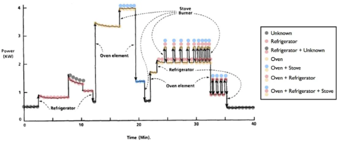
On the one hand, event-based approaches are intrinsically related to the early days of NILM, and seek to disaggregate the total consumption by means of detecting and labeling
every appliance transition in the aggregated signal (see in Figure 2.1) using previously trained
supervised or semi-supervised learning algorithms. Consequently, approaches categorized
under this category require a data collection step where a number of transitions (i.e., power
events) from the appliances of interest are collected, labeled and stored, to be used later as
training data.
5
1st International NILM Workshop, www.ices.edu/psii/nilm
Appliance type Description Examples
ON / OFF Appliances that are either running or not, i.e. either ON or OFF.
Light-bulb, toaster and water kettle
Finite State Appliances that during their operation will pass through a finite number of operation modes.
Clothes washer and clothes drier
Variable Power Appliances whose power draw is variable and no finite
number of states or transitions can be observed. Dimmer lights and power tools
Permanent Consumers
Appliances that normally run on the background 24/7 with constant power draw.
Figure 2.1 – Example of event-based energy disaggregation
Event-less approaches, on the other hand, do not rely on event detection and classification. Instead, these approaches attempt to match each sample of the aggregated
power with the consumption of one specific appliance or a combination of different
appliances (see Figure 2.2), by means of statistical (e.g., Bayesian methods) and probabilistic
(e.g., Hidden Markov Models) machine-learning methods. Therefore, the training data does
not require any labeled transitions. Instead, only the aggregated consumption of the loads of
interest is required. Thus making the process of collecting training data for event-less
approaches more straightforward than for event-based approaches.
Figure 2.2 – Example of event-less energy disaggregation
Naturally, both approaches have advantages and disadvantages. For example, despite the
fact that event-based approaches require the continuous execution of event detection
making these approaches more computationally efficient. Yet, the success of the final energy
estimation is heavily dependent on the detection and classification steps, consequently, any
missed detections or erroneous classifications will be propagated in time, possibly leading to
large energy estimation errors.
On the other hand, in the case of event-less approaches, the inference step is performed
for every sample, making such approaches considerably more computationally intensive.
Nevertheless, since all the data is taken into consideration at all times, errors are not expected
to propagate. Instead, these will be corrected as the inference algorithms are being executed.
2.3
Existing Challenges
More than three decades after Hart first introduced Non-Intrusive Load Monitoring in his
seminal work [13], this is still a very active field of research. Yet, despite all the research
efforts, to date some considerable technical challenges are still present.
Currently, the different challenges are grouped according to two categories, namely: i)
load identification challenges; and ii) training and supervision challenges [21]. These are
described next in more detail.
2.3.1
Load identification challenges
Challenges under this category are related to the problem of correctly identifying the
individual loads, and the first challenge is the ever-growing complexity of the domestic
electric grid and the very different load types [24], [25] that NILM systems must account
for. For instance, variable power loads (e.g. dimming lights), multistate loads (e.g. clothes
washer) and always-on loads (e.g. security cameras and alarms).
Likewise, NILM algorithms also need to be able to discern between appliances that
draw the same power [24], [25], independently of being similar appliances or just different
devices working at the same power level. Furthermore, and more specifically for event-based
approaches, researchers need to account for simultaneous power events (i.e., when loads are
detection process that can propagate to the subsequent stages and result in large energy
estimation errors [32].
Lastly, and perhaps the most important challenge, is the fact that researchers need to be
fully aware of the dynamic nature of the electric grid [33], which makes the problem of
energy disaggregation considerably different from many other classic machine-learning
problems. In other words, in many of the classic machine-learning domains (e.g., speech
recognition or hand writing recognition) training and testing datasets are assumed to have the
same or nearly the same statistical properties of the future data that will be given to the
learning algorithms. However, due to the dynamic nature of the electric grid, this is not likely
to happen in NILM problems. Instead the learning algorithms must be robust against changes
in the future data, like for example the presence of unknown and / or malfunctioning
appliances or the many different modes of operating and combining such appliances [16],
[34].
2.3.2
Training and supervision challenges
Challenges under this category encompass the many issues related to training and evaluating
the performance of the different NILM solutions that are being proposed by the research
community. For example, different algorithms require different training data, e.g.,
event-based approaches need labeled transitions while event-less approaches require historical
traces of individual appliance consumption data. Yet, very little work was carried out in this
direction, thus there are currently no identified strategies to collect training data [25], [33].
This is especially important in the case of event-based approaches as these rely on
considerable amounts of labeled appliance transitions that will most probably require human
intervention to get.
Furthermore, and despite the efforts to create public datasets that is being observed in the
last couple of years, the shortage of proper public datasets is still considered one of the
main caveats of NILM research, particularly in the case of fully labeled datasets that are
required to train and validate event-based approaches. Moreover, the currently available
measurements, data resolution and appliance types), which on the one hand makes the task of
evaluating algorithms very time consuming, and on the other hand, adds considerable bias to
the evaluation results, hence compromising any cross-dataset benchmarks.
Finally, and despite some efforts that have been made to carry out formal evaluations of
the technology (e.g., [27], [31], [36]), as of today there is no formal agreement on which
metrics should be used to measure and report the performance of NILM algorithms and
systems [31]. Instead, most evaluations have focused solely on reporting the accuracies of the
proposed methods without having previously studied the compliance between the used
metrics and the NILM problem, like it is done in other machine-learning domains [37], [38].
2.4
Literature Review on Load Disaggregation
As it was mentioned previously, as of today the different approaches to the NILM problem
are grouped according to two categories, namely: event-based and event-less approaches. As
such, in the next two sub-sections we summarize some of the most relevant research to date
according to these categories. Nevertheless, we should note that other categorizations can be
found in the literature, for example [24] categorizes NILM research in terms of the metering
feedback dimension, i.e. low frequency vs. high frequency, while [25] focuses on signature
features and algorithms.
2.4.1
Event-based Approaches
Event-based approaches for energy disaggregation are intrinsically linked to the early work
by Hart, and aim at computing individual appliance consumption by keeping track of every
appliance state transition (e.g. kettle turning ON or OFF) by means of event detection and classification assuming that the system was previously trained.
A typical event-based NILM system workflow contains five consecutive steps, as shown
in Figure 2.3: data acquisition, where signals representing the electrical energy flowing into
the house are sensed, sampled and transformed into power-related measurements (e.g. real
the consumption that are assumed to happen in response to appliances changing their mode of
operation; iii) feature extraction, where different parameters are extracted from the vicinity
of the power event, forming a power event signature that will be used in the process of
identifying the loads responsible for each event; iv) event classification, where previously
trained machine-learning algorithms are applied to the signatures of the previously detected
power events to obtain a classification, i.e., the name of the appliances that triggered the
events; and v) energy estimation, where the consumption of the individual loads is estimated
based on the labeled power events and their distribution in time. Next, we provide a
comprehensive literature review on the event detection, feature extraction, event
classification and energy estimations steps.
Figure 2.3 – General workflow for event-based NILM approaches
2.4.1.1
Event detection
According to the literature in event detection for NILM [39], the different approaches are
grouped in three categories: i) expert heuristics; ii) probabilistic models; and iii) matched
filters.
Expert heuristics
Algorithms under the expert heuristic category are probably the less complex, and follow the
basic principle of scanning the time series data looking for changes that are above a certain
threshold, as defined by Hart is his seminal work [13].
For example, in [40] the power signal is first filtered to minimize the presence of noise
and reduce the chance of false positives. On a second step, the power events are detected by
means of computing the absolute differences between two consecutive samples and selecting
the indexes where this difference is above a pre-defined threshold. In [41] a similar approach
samples, the differences are calculated between the current sample and the sample X seconds before. Moreover, in order to help reduce the number of false positives, an index with
absolute value above the pre-defined threshold is only considered a power event if no power
event was detected in the last Y seconds.
Probabilistic models
Another approach to event detection is by means of probabilistic methods. In this category of
detectors, the event detection occurs in two steps, as described below:
In the first step it is necessary to calculate the chance of an event occurring at each
sample of the power signal. This signal is normally referred to as the detection statistic, and is computed by applying either statistical tests (e.g., Generalized Likelihood Ratio (GLR) [42],
Goodness-of-Fit (GOF) [43], CUmulative SUM (CUSUM) [44]) or other mathematical
functions (e.g., Kernel Fisher Discriminant Analysis (KFDA) [45]), to the power
measurements by means of sliding windows.
In the second step the power events are extracted from the resulting detection statistic
signal. This is normally done via thresholding, i.e., whenever the detection statistic is above a
certain threshold a power event is flagged in the power sample that corresponds to that index
[42], [43]. Nevertheless, for the particular case of NILM, more robust strategies have been
designed. For instance, in [46] and [47] the selection of the power events is done by applying
either a voting algorithm or a maxima/minima locator algorithm to the detection statistic
signal, respectively.
Match filters
In this category of algorithms, power events are detected by correlating a known, or template
with an unknown signal to detected the presence of the former signal in the later. In other
words, match filter event detectors work by trying to find known appliance transients (i.e.,
templates) in the aggregated consumption signal (i.e., unknown signal) by means of filtering
techniques.
To the best of our knowledge, this was first attempted in the NILM domain in [44] and
transients (obtained from training) to the aggregated signal using two transversal filters in
sequence. The first filter is used to find the transient shapes in the aggregate signal, and the
second filter is used to enforce that the matches correspond to actual transients and not some
fortuitous noise [49].
As of today, the match filters category also incorporates those detectors that use filters to
transform the power measurements into signals that emphasize potential power events while
depreciating the steady stage regions, similarly to what is done in the probabilistic models
category. For example, in [50] the authors apply a Hilbert transform6
to the instantaneous
current sampled at 20 kHz. This is followed by a combination of average and derivation
filters on the transformed signal such that only the transitions of interest (i.e., power events)
are represented.
Another example of event detection based in filter matching is the work of Baets et al.
[51] that apply Cepstrum analysis7 to the power signal computed at 60 Hz. The resulting
signal is then thresholded such that only the positions where the signal is above a certain
value are considered power events.
2.4.1.2
Feature extraction
Feature extraction is the process of selecting the best features such that the power event
signatures are robust and have enough discriminative power between different appliances.
Overall, features can be categorized as being either engineered features or data driven features. The former encompasses features that are extracted by taking advantage of the domain knowledge that we have from electrical power and appliance characteristics while the
latter refers to features that are learned directly from the data by means of techniques like
unsupervised feature learning [52].
Engineered features are normally extracted from the samples surrounding the event of
interest. The most common examples of these features are the amount of power change (also
known as delta metrics), transient shapes, harmonic components [46] and voltage and current
6
Hilbert transform, http://mathworld.wolfram.com/HilbertTransform.html 7
(V-I) trajectories [53], [54]. Additionally, several features have been drawn from the
frequency domain content like Electromagnetic Interference that emanate from certain
appliances [55], electric noise [56] using Fast Fourier Transforms (FFT) or in some cases the
Wavelet transform to simultaneously extract time and frequency domain features [57].
With respect to data-driven features, these are also extracted from the measurements
surrounding the power event. Yet, unlike engineered features, these are directly learned from
the data. For example, in [54] Lam et al. proposed the application of Single Value
Decomposition (SVD) techniques to extract features from the current waveforms, whereas
Gao et al. propose the use of VI binary images (V-I trajectories that are amplitude normalized
and converted to binary images) and Principal Component Analysis (PCA) on the V-I binary
images [58].
2.4.1.3
Event classification
Current NILM literature is very rich in terms of supervised learning algorithms for event
classification. These range from the more traditional learning algorithms, like the K-Nearest
Neighbor (K-NN) [44], decision trees [58], [60], naïve Bayes (NB) [61], [62], artificial
neural networks (ANN) [63], [64], [65] or support vector machines (SVM) [60], [66], [67] to
more complex approaches like genetic algorithms (GA) [60], [63], [68] and Integer
programming [69].
Some authors have also explored the feasibility of ensemble-based approaches where
different algorithms are combined to enhance the overall classification performance [70],
[71], Likewise, the possibility of sequentially combining different classification algorithms
was also explored. For instance, in [41] the authors propose a two-step approach for energy
disaggregation. In the first step, one classifier attempts to discriminate the appliance by
category (i.e., purely resistive, inductive or capacitive), such that in the second step another
classifier is trained with only the features that are considered relevant to identify appliances
under that category.
Lastly, Barsim and Yang have also experienced with semi-supervised approaches that
[72]. In very simple terms, the rationale behind semi-supervised approaches is the fact that in
most machine-learning problems labeled data is scarce or very expensive to obtain. As such,
semi-automatic learning methods attempt to leverage the potential of unlabeled data by using
small sets of labeled examples to infer the labels of unlabeled examples and use them later as
training data [73].
2.4.1.4
Energy estimation
Finally, in the energy estimation step the classified power events and associated timestamps
are used to infer the consumption of the individual appliances. This topic was briefly
explored in Harts original work where the author proposes to model the individual appliance
consumption be means of expert heuristics like the Zero Loop Sum Constraint (ZLSC), which
states that the sum of power changes in any cycle of state transitions is zero [14]. This
method, however, is simplistic given that it assumes that power transitions of a given
appliance are symmetrical, and that there are no simultaneous events.
Other attempts on the topic of energy estimation include the works of Baranski and Voss
[68], [74] and Streubel and Yang [75]. The former presents a completely unsupervised
method of estimating appliance behavior based on observed power differentials, and
optimization of a quality function using genetic algorithms (GA). The later proposes the
modeling of appliance behavior using Finite State Machine (FSM) formulations by separating
the power traces of a single appliance into transients and steady-state modes. However, these
two approaches remain to be validated and some of the assumptions made by the authors
have been shown to present some considerable drawbacks to both approaches as stated in
[24] and [76].
Lastly, Giri and Bergés also proposed an approach to energy estimation [76]. The
proposed framework that aims reducing the effects of outliers (incorrect labels) and missed
state transitions, is composed of five sequential steps: i) clustering of the detected power
events, ii) perturbation of the power events to enforce the ZLSC, i.e., correction of the missed
that violate the ZLCS, i.e., correction of outliers, and v) estimation of energy consumption
using the resulting FSMs of each individual appliance.
The proposed framework was tested on the BLUED [77] and REDD [78] datasets, using
the percentage error in energy estimation (PEEE) [46] as the performance metric. The results
have shown a considerable variation of the performance metric across the datasets, which in
average ranged from 5.9% and 16. 5 in BLUED to 22.4 in REDD.
In summary, the sequential nature of event-based approaches implies that each step in the
process will result in affecting its successors. Consequently, it is safe to say that the ultimate
goal of these solutions is to find the best combination of algorithms and features across the
different steps such that the properly disaggregated energy is maximized. Furthermore, it is
evident that these approaches require big volumes of labeled data for algorithm training,
which in itself is another different problem for NILM researchers to solve.
To the best of our knowledge, as of today, only a few authors have attempted to tackle
this issue. For example, Berges, in his user-centered approach, provides a mechanism that
prompts users to provide appliance information whenever the system is not able to find a
match with a power event [46]. Weiss [59] proposes the application of mobile apps in order
for users to collect appliance labels and signatures in real time. Lastly, on the commercial
side, Bidgely proposes the application of crowdsourcing techniques to collected appliance
labels from their customers [79].
2.4.2
Event-less Approaches
Unlike event-based approaches, the event-less alternatives do not require that
machine-learning algorithms be previously trained to identify every individual power change in the
aggregated signal. Instead, these approaches rely mostly on the existing knowledge about
individual appliance operation, through different techniques like motif mining, blind source
2.4.2.1
Motif mining
A motif mining approach for energy disaggregation was proposed in [80] and works by
mining the aggregated power signal for recurring episodes (i.e. individual appliance working
cycles), that are composed of sequences of power events ( e.g. + 1000 -400 -600) and match
them to individual devices that are known to exhibit such behavior. Each episode must fulfill
certain conditions in order to be considered as belonging to an appliance. This includes the
minimal episode completion criterion that is used in order to identify episodes that are
completed by a single device (e.g. the episode +600 -800 +400 -1000 + 800 would not be
considered, whereas episodes +600 +400 –-1000 and -800 +800 would be accepted).
2.4.2.2
Blind source separation
Blind source separation is the process of separating individual sources from a signal that is
known to be composed of a set of mixed signals but very little or no information is provided
regarding the source signals or the mixing process.
In [81], a blind source separation technique has been applied to the problem of energy
disaggregation where the authors use the steady-state active and reactive power changes (∆P and ∆Q) to create appliance clusters, each of which was assumed to correspond to one appliance state transition. A matching pursuit algorithm (MP) is then applied to reconstruct
the original source (i.e. aggregated power) of each cluster (i.e. appliance). Another example
of blind source separation is presented in [82] where the authors propose the application of
discriminative sparse coding to find the sets of basis functions that best represent each
individual appliance. Non-negative matrix factorization is then applied to find the optimal
sparse set of basis function activations that best explain the household aggregate data.
2.4.2.3
Probability graphical models
In contrast to the methods we have seen so far, that require a separate event detection process,
a new approach has emerged in which load disaggregation is attempted using probabilistic
the power consumption and eventually non-power features such as the duration and time of
appliance usage.
The basic assumption behind such methods is that the aggregated electrical energy
consumption (P) at a given instant (t) is characterized by the consumption of several
appliances that are operating in a particular mode. Therefore the disaggregation problem can
be formalized as the task of finding the best possible mode sequences (m) that explain the
observed aggregated power (P). Given this, authors have attempted to develop such models
of appliance behavior using several variations of Hidden Markov Models (HMM), in which
the ultimate goal is to find the sequence of hidden states that best represent the model outputs
(i.e. the aggregate power at a given instance in time).
An example of using HMM for energy disaggregation is the work of Parson et al. in[83]
in which, for each appliance, a semi-supervised algorithm is used to determine its most likely
sequence of states (i.e., model each appliance as a HMM). To that end, the authors feed their
modeling algorithm with generic appliance models containing information about the
operational characteristics of the appliance type they are modeling (e.g., aggregate
consumption, state transition probabilities and the estimated consumption in each state).
Lastly, using the state sequence of each appliance the disaggregation algorithm attempts to
estimate its consumption and subtract that from the aggregated consumption before repeating
the process for the next available state sequence, until there are no more state sequences
remaining.
Likewise, Kolter and Jaakkola [84] also propose modeling appliances as HMMs, yet, in
contrast to Parson et al. [83], the authors use an unsupervised algorithm to estimate the
number of appliances and their consumption patterns taking only the aggregate consumption
data as input. To this end, the algorithm works by extracting snippets of the aggregated
consumption data that most likely correspond to an appliance s working cycle (defined as the
period between the appliance s start-up and shutdown). Each extracted snippet is then
modeled as an HMM and those that are most likely to belong to the same appliance are
identified as such. This results in a factorial HMM (FHMM) (i.e., a composition of several
independent HMMs), which the authors then use to estimate the consumption of the