1
A Work Project, presented as part of the requirements for the Award of a Master Degree in
Economics from the NOVA – School of Business and Economics.
House Price Cycles in Europe
Joana Gabriela Costa Ferreira Leiras, number 829
A Project carried out on the Master in Economics Program, under the supervision of:
Professor Paulo M. M. Rodrigues
2 Abstract:
This Project uses data for GDP and real housing prices for twelve European countries plus the
United States to study the relationship between the housing market and GDP cycles. The main
findings suggest that there is evidence of a strong relationship between the two cycles for most of
the countries analysed. Moreover, an analysis of the relationship between the Portuguese economy
and other European economies is also performed for the two cycles. This analysis shows that there
is a strong correlation between the European economies when the GDP is used as benchmark and
that this correlation decreases when the housing market is considered.
Key Words: Housing price cycle, GDP cycle, Synchronization and Convergence, European Union
Acknowledgements: I would like to thank Raul Guerreiro for his very helpful contribution in
the making of this project and to professor Paulo Rodrigues for his orientation and support
without which this would never be possible. Moreover I would like to thank my family for their
3 1. Introduction
The strong recession that occurred in the US in 2008 as a result of a housing market crash
brought up chaos all across the globe in a way that many perceived as the worst global recession
since World War II. As stated by Verick and Islam (2010) the effects of this global recession differ
largely among countries depending mostly on the state of the economy prior to the burst of the
housing market bubble. Among the European Union, the vast majority went through a long-lasting
period of economic contraction as a consequence of the big decrease in household’s wealth and a
rise in unemployment which contributed to the fall of the average GDP all around Europe as
referenced by Buti et al. (2009). This was particularly felt by middle-income countries in central
and eastern Europe such as Lithuania, Latvia and Estonia.
Given the level of integration inside the European Monetary Union it is of great importance to
study how the involved countries are related among each other. A lack of synchronization among
these countries could lead to unforeseen effects caused by economic policies. Monetary policy
plays an important role in shaping the housing market. This responds negatively to contractionary
monetary policy shocks which causes significant effects on the housing market.
The devastating effects of the burst of this house prices bubble intrigued many economists into
studying this market more closely. Some of the most common research points in this market
consists of how it relates with the GDP cycle and its main components2. This project studies both
of these problems. In a first approach, the GDP and house price cycle will be used to study the
level of correlation between the two cycles. For robustness, this calculation will be computed across
various European countries plus the United States. In a second approach, the level of correlation
2
4
between the Portuguese economy and several other European economies will be analysed. Besides
studying the relationship inside the European Union a comparison of the Portuguese cycles and the
ones from the United States is also provided.
This project is organized as follows: in section 2 there is a review of the literature already
produced on the topics evaluated in this paper; section 3 presents the main procedures applied
throughout this project and the data used; section 4 discusses the results and, finally; section 5
provides the main conclusions derived from this analysis.
2. Literature Review
The shocking effects caused by the 2008 housing market crash generated a sudden concern on
this market. Since then, many studies have been conducted in order to better understand its
behavior. Using a structural VAR, Iacoviello and College (2002) found that “housing price
inflation is highly sensitive to forces driving economic fluctuations” which might be an indicator
of a high correlation between house prices and GDP.
The high level of correlation between GDP and housing market cycles is found to be true in
several European economies. Using data from the French economy, Ferrara and Vigna (2010)
found that there are high correlation levels between GDP and several housing market variables like
household investment. Moreover, there is also evidence of a high correlation between the
household investment and housing prices which, by association, can lead to evidence of correlation
between housing prices and GDP. Similar conclusions were drawn by Álvarez and Cabrero (2010)
for the Spanish economy and by Bulligan (2009) for the Italian economy. Both found evidence of
a high correlation between both the housing investment and GDP and between the housing
5
and GDP these three authors’ findings are no longer in accordance. While in Italy housing prices
are found to be lagging GDP by 2 years, in France housing prices tend to lead the economic cycle
by 2 quarters. In Spain, the results are found to be somewhat inconclusive since the two filters used
in the analysis provide two different results. When the Butterworth filter is used, the two cycles are
found to be in line with each other while, when using the Epanechnikov filter, the house price cycle
is found to be lagging GDP by 4 quarters.
The level of synchronization among the countries integrated in the European Monetary Union
(EMU) is one of the most important criteria for an optimal economy. As such it is of great
importance to study how these countries are related to each other. Using a dynamic factor model
Kose et al. (2008) found evidence of an increase in convergence among industrial economies
during the globalization period. These findings are aligned with the ones provided by Ferroni and
Klaus (2015) which suggest a high level of interdependence between Germany, France and Italy
while Spain seems more dependent on domestic factors. Using a cross correlation analysis similar
to the one used in this project, Álvarez et al. (2010) also concluded that, when using GDP as a
variable of comparison, there is a high level of correlation between those same economies.
Moreover Mink et al. (2008) using synchronicity and co-movement measures found a high
correlation between business cycles in France, the Netherlands, Spain and Germany while Ireland
and Greece show a lower correlation with the remaining EMU countries.
Through the use of a Markov-Switch model, Corradin and Fontana (2013) showed that house
price returns are better characterized as having three phases, a high, low and medium phase which
differ largely across countries though this difference has been decreasing since the beginning of
the century. However, Álvarez et al. (2010) performing a correlation analysis using the housing
6
this variable is used rather than when GDP is used which suggests that, unlike the GDP cycle, the
housing market is more dependent on idiosyncratic characteristics.
3. Methodology
A wide range of different procedures has emerged in order to study the housing market cycles.
In this project, the procedure applied is one similar to the one used by Álvarez et al. (2010) which
consists in analyzing several metrics like the correlation measure, the concordance index (CI) and
the cross-correlation index (CCI) in order to access how the GDP cycle relates to the housing
market cycle and also infer on how the Portuguese economy relates to each of the remaining
countries based on both GDP and real house prices.
The economic cycle can be interpreted as a combination of three major components as proposed
by Clark (1987). These components are: the trend, which represents the direction that the economy
is pursuing in the long-run; the cycle, which corresponds to the short-term fluctuations; and the
irregular component, which accounts for unpredictable fluctuations around the trend.
𝑌" = 𝑇"+ 𝐶"+ 𝜀"
There are several methods used to represent both the trend and the cyclical components. In this
project the trend is assumed to be a combination of two variables, a trend (𝛽") and a level (Γ") which
follow a random walk process as presented by Gilchrist (1976) while the cycle is assumed to follow
a second order autoregressive process AR(2) as proposed by Clark (1987). This model can be
represented as
𝑦"= Γ"+ 𝐶"+ 𝜀"
Γ" = Γ"+,+ 𝛽"+,+ 𝛿"
𝛽" = 𝛽"+,+ 𝜃"
7
There is a vast number of procedures used to separate a data series in its cyclical and trend
component being some of the most widely used the Hodrick and Prescott’s and the Baxter and
King’s Filter. The HP Filter is a high-pass filter that splits the trend from its cyclical component by
minimizing the deviations from the trend given a predetermined business cycle component. This
filter removes the higher frequency fluctuations as part of the cyclical component and retains the
smaller ones as being part of the trend(see De Haan et al. (2010)). Meanwhile, the Baxter and King
filter proposed by Baxter and King (1999) uses a moving average to isolate the periodic
components which lie in a specific band of frequencies.
In this project, the method used to extract the cycle from the series is the Kalman filter. The
Kalman filter uses a Bayesian approach in the sense that it is updated recursively using current and
past information to infer on the next period forecast. This filter provides minimum mean square
estimators using a least-square procedure. Following Pasricha (2006) let us consider a simple
model, such as,
𝑍"= 𝐻′"𝑋"+ 𝑣" , 𝑋"9, = 𝐹"𝑋"+ 𝑤"
𝑌"= 𝑇"𝑋"+ 𝜀" , 𝑋"9, = 𝐹"𝑋"+ 𝜂"
where 𝑋" represents the unobservable variable(s) and 𝑍" is the observed variable. 𝑤" and 𝑣" are
the noise components and are assumed to be white noise and independent. The Kalman filter
provides estimations of 𝑋"|"+,= 𝐸 [𝑋"|𝑍"+,] and 𝑋"|" = 𝐸[𝑋"|𝑍"] with covariance matrix
Σ"|"+,and Σ"|" respectively and can be expressed as
𝑋"9,|" = [𝐹"− 𝐾"𝐻D"]𝑋"|"+,+ 𝐾"𝑍"
8
A final remark regarding the Kalman filter is related to the initialization process which is
assumed to be unknown. Across several existing techniques, the one used in this project is the one
presented by Durbin and Koopman (2001) which assumes that some of the state elements might
be nonstationary. This method its called diffuse initialisation and provides estimates for the
unknown parameters, here defined by q, through the maximization of the diffuse likelihood
𝑙og𝐿 𝒀 𝛉 = −1
2 𝑙𝑜𝑔 2𝜋 𝑭" + 𝒗"
D𝑭 " +,𝒗
" S
TUV9,
The fact that the Kalman Filter updates itself at each point in time implies that it uses all the
information available at each point in time to predict the unobservable values. This feature
represents one of the major advantages of this approach.
De Han et al. (2007) provide an analysis of the pros and cons of using different filtering
techniques and the main conclusions drawn were that, in most cases, standard filters are found to
provide similar results.For robustness purposes, the decompositions using the HP and the Baxter
and King filters will also be performed to infer whether they provide similar conclusions to the
ones obtained using the Kalman filter.
In order to assess the relationship between two series several metrics will be computed. One of
the metrics applied for this purpose is the Pearson correlation. This measure consists of a simple
correlation measure which takes values between -1 and 1 where -1 means perfectly negatively
correlated, 1 perfectly positively correlated and 0 meaning not correlated.
A second measure used is the Concordance Indicator (CI) proposed by Harding and Pagan
(2002) which computes the synchronicity between two series using a binary indicator to assess the
9
series will undergo a two-step procedure. The first step consists in converting each of the two series
in a sequence of -1 and 1 where it acquires a value of 1 when the series is increasing from one
moment to the other and -1 when it is decreasing. The second step consists in comparing the two
series at each point in time and creating a binary sequence where it presents a value of 0 whenever
the two are not in the same phase and 1 when they are in the same phase, same phase meaning
either both increasing or both decreasing.
One last measure included in this project is the Cross-correlation Index (CCI) which gives us
the number of periods by which one of the cycles is leading or lagging the other. This measure is
calculated through an analysis of the various cross-correlation values between two series across a
twelve-period horizon, both leads and lags. The period where the correlation value reaches its
maximum is the one that provides the number of periods by which one series is leading or lagging
the other (see Backus et al. (2016)).
3.1Data
This project performs two different analysis, the first one is on the correlation between the
house price cycle and the GDP cycle and the second one is the correlation between Portugal and
the remain economies regarding these two cycles. To do so, logarithmic data for the real house
price and GDP is used for thirteen countries: Austria, Belgium, Finland, France, Germany, Greece,
Ireland, Italy, Netherlands, Portugal, Spain, UK and US. The time period used in this analysis
differs across countries, due to data availability constrains. The majority of the analyzed countries
has data from 1970Q1 until 2015T4 except for Spain which has available data from 1971Q1 to
2015Q4, Austria from 1986Q3 until 2015Q4, Portugal from 1988Q1 until 2015Q4 and Greece
which only has data available from 1997Q1 onwards. It is important to remark that the data series
10
by Knetsch (2009) might lead to unreliable conclusions since the housing market suffered several
changes during that period of time.
Throughout this analysis the data constraints for each of these regions is taken into
consideration when comparing to series with different data lengths. In this cases the length
considered is the one from the shortest series which is the case, for example, when comparing the
GDP and the housing price cycle between Portugal and the remaining countries, because the period
of data available for Portugal is lower than the one from the remaining countries, the data length
considered is from 1988Q1 until 2015Q4. Due to a low number of observations, the comparison
between the Portuguese cycles and the Greek cycles will not be computed.
4. Results
4.1. GDP and Housing Cycle correlation analysis
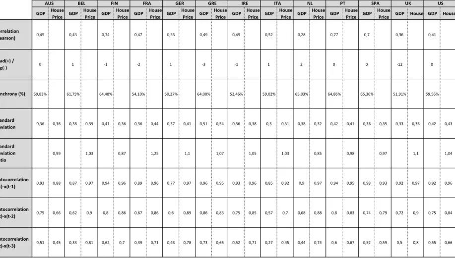
This first section provides a discussion of the results obtained from the correlation analysis
between the GDP and House price cycles for each individual country. The main results from this
analysis are represented in table 1.
The Pearson correlation values obtained from this analysis show evidence of a high level of
correlation between the GDP and the house prices in the vast majority of the countries. These
values are found to be positive for all countries included in our sample which implies that, even if
in a small scale, house prices and GDP move in the same direction. The values for the analyzed
countries range between 0,28 and 0,77 where the highest values are found for Portugal with 0,77
Spain 0,7 and Finland with a 0,74 correlation value. The lower values are found for the Netherlands
11 Table 1: GDP vs House Price
GDP House Price GDP
House Price GDP
House Price GDP
House Price GDP
House Price GDP
House Price GDP
House Price GDP
House Price GDP
House Price GDP
House Price GDP
House
Price GDP House GDP House Correlation
(Pearson) 0,45 0,43 0,74 0,47 0,53 0,49 0,49 0,52 0,28 0,77 0,7 0,36 0,41
Lead(+) /
Lag(-) 0 1 -1 -2 1 -3 -1 1 2 0 0 -12 0
Synchrony (%) 59,83% 61,75% 64,48% 54,10% 50,27% 64,00% 52,46% 59,02% 65,03% 64,86% 65,36% 51,91% 59,56%
Standard
Deviation 0,36 0,36 0,38 0,39 0,41 0,36 0,36 0,44 0,37 0,41 0,51 0,54 0,36 0,38 0,3 0,31 0,38 0,32 0,42 0,41 0,36 0,35 0,33 0,36 0,42 0,43 Standard
Deviation Ratio
0,99 1,03 0,87 1,25 1,1 1,07 1,05 1,03 0,85 0,98 0,97 1,1 1,04
Autocorrelation
x(t)-x(t-1) 0,93 0,88 0,87 0,97 0,94 0,96 0,89 0,96 0,77 0,97 0,96 0,95 0,93 0,96 0,85 0,92 0,9 0,97 0,94 0,95 0,93 0,93 0,92 0,97 0,92 0,96 Autocorrelation
x(t)-x(t-2) 0,75 0,66 0,62 0,9 0,8 0,86 0,67 0,86 0,6 0,89 0,86 0,83 0,75 0,85 0,57 0,7 0,68 0,88 0,8 0,83 0,74 0,79 0,72 0,9 0,75 0,84 Autocorrelation
x(t)-x(t-3) 0,51 0,45 0,33 0,81 0,62 0,7 0,39 0,71 0,43 0,78 0,73 0,65 0,52 0,71 0,27 0,45 0,44 0,74 0,6 0,67 0,52 0,59 0,5 0,8 0,55 0,66 US
IRE ITA NL PT SPA UK
12
The second variable analyzed is the Concordance Index (CI) proposed by Harding and Pagan
(2002). The conclusions drawn from this measure are similar to the ones provided by the Pearson
correlation, which is that there is indeed a high level of synchronicity between the two cycles. All
countries show synchronicity values above 50% being the lowest ones Germany with a CI of
50,27% and the UK where there is a synchrony of 51,91% between the cycles. The higher
synchronicity values are found in Austria, Spain and the Netherlands with values slightly above
65%.
Lastly the cross-correlation index provides us with information on whether the house price
cycle is leading or falling behind the GDP cycle. The conclusions drawn from it, contrary to the
previous ones, vary from country to country. There is a slight lead of the housing cycle towards the
GDP cycle in countries like the Netherlands, where there is a 2-period lead towards GDP and,
Germany, Italy and Belgium where there is a 1-period lead. The results obtained for the Italian
economy contrast with the ones obtained by Bulligan (2010) who found evidence of a 2-year delay
between the real house prices and GDP. In some other countries like Austria, the US and the Iberian
countries, the two cycles are found to be synchronized with each other. Comparing these results
with the ones obtained by Álvarez and Cabrero (2010) for the Spanish economy, these ones confirm
the results provided by the Butterworth filter which found evidence of a contemporaneous
relationship between the two cycles. Greece and France show a 3 and 2 trimester lag towards GDP
respectively while Ireland and Finland show a 1 period lag. The results found for France also
contradict the ones found by Ferrara and Vigna (2009) who found evidence of a 2-period lead
between the housing market and GDP. The biggest outlier in this analysis is the UK which shows
a 3-year lag between the two cycles. These findings are consistent with the ones drawn from the
13
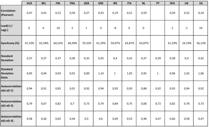
4.2. Portugal vs Other Countries Correlation Analysis
So far, it has been shown that there is indeed a correlation between the GDP and the house price
cycles, even though not very significant in some of the analyzed countries. Another important issue
raised in the course of this project is whether there is a relationship between countries. In this
section, such an analysis will be computed for the Portuguese economy by looking at how the two
variables in this economy relate to the ones from other economies. The results obtained from the
analysis on the GDP cycle are summarized in table 2.
Looking at the Pearson correlation values obtained in this analysis, there is evidence that GDP
in some countries is correlated with the Portuguese one. Among these countries are Spain and the
Netherlands with a correlation level of 0,59. Other countries like Germany and Italy also show a
high correlation level with the Portuguese economy as far as GDP is concerned. Contrary to the
Table 2: Portugal vs Other Countries (GDP approach)
AUS BEL FIN FRA GER GRE IRE ITA NL PT SPA UK US
Correlation
(Pearson) 0,47 0,42 0,22 0,34 0,57 0,43 0,19 0,51 0,59 0,59 0,32 0,18
Lead(+) /
Lag(-) 0 0 -10 -1 1 -2 -8 0 0 -1 -1 10
Synchrony (%) 67,10% 62,58% 64,52% 68,39% 70,32% 61,29% 50,97% 63,87% 63,87% 61,29% 54,19% 56,13%
Standard
Deviation 0,37 0,37 0,37 0,36 0,35 0,45 0,4 0,41 0,37 0,39 0,38 0,4 0,42
Standard Deviation Ratio
0,95 0,94 0,93 0,91 0,89 1,14 1 1,05 0,95 1 0,96 1,03 1,06
Autocorrelation
x(t)-x(t-1) 0,94 0,91 0,95 0,91 0,92 0,94 0,95 0,93 0,88 0,92 0,95 0,94 0,92
Autocorrelation
x(t)-x(t-2) 0,79 0,67 0,82 0,7 0,73 0,79 0,84 0,75 0,68 0,72 0,82 0,78 0,73
Autocorrelation
14
previous, some other countries show very low values of correlation although still positive. Among
the European nations, we find that Ireland and Finland are the regions with the lowest correlation
with the Portuguese economy with correlation values of 0,19 and 0,22 respectively. For the United
States, the correlation seems to be even lower than in the rest of the countries which might suggest
a low correlation of economic cycles between the US and the European Countries.
The Concordance Index (CI) shows high levels of synchronicity between the Portuguese and
the remaining countries GDP. This is particularly clear in Germany where the two cycles are found
to be moving in the same direction more than 70% of the times. France and Austria also show high
levels of synchronization with the Portuguese economy, 68,87% and 67,10% respectively. In line
with the results obtained from the Pearson correlation, Ireland and the US appear to be the ones
less synchronized with the Portuguese economy, even though still showing high values of
synchronicity.
Regarding the cross-correlation analysis, some of the conclusions are also in line with the ones
obtained in the two-previous analysis. Both Ireland and the US are found to have cycles far apart
from the Portuguese one. While Ireland is lagging the Portuguese economy by a 2-year period, the
US economy is leading the Portuguese economy by 10 quarters. Finland also shows a big lag
towards the Portuguese economy which confirms the findings from the Pearson correlation.
Moreover, countries showing high values of correlation are found to be more aligned with each
other. This is evident in countries like Netherlands and Italy. Germany, which was found to be the
country with the highest synchronicity with the Portuguese economy, is found to have a 1-period
lead on the Portuguese economy, being also the only European country leading the Portuguese
15
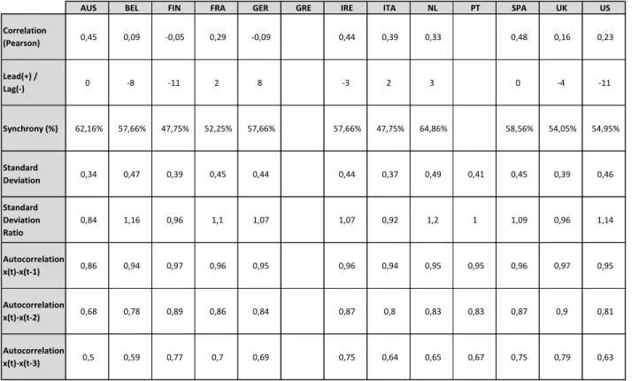
After analyzing the GDP cycle correlation between Portugal and the remaining countries, this
section provides now a new correlation analysis, this time using the real house price cycle as
comparison. The results of this analysis are summarized in table 3.
The conclusions drawn from the Pearson correlation in this new analysis are not as evident as
they were for the GDP cycle. Overall, the values are found to be lower than the ones obtained
previously plus there are also some cases where values fall below zero. This is true for Germany
and Finland which show correlation values of -0,09 and -0,05 respectively. This negative values of
correlation mean that, not only there is there a low correlation between the two, but also that the
two cycles move in opposite directions, in other words, when the house price cycle is increasing in
Portugal, in Germany and Finland it is decreasing. Contrarily to Germany and Finland, Spain,
AUS BEL FIN FRA GER GRE IRE ITA NL PT SPA UK US
Correlation
(Pearson) 0,45 0,09 -0,05 0,29 -0,09 0,44 0,39 0,33 0,48 0,16 0,23
Lead(+) /
Lag(-) 0 -8 -11 2 8 -3 2 3 0 -4 -11
Synchrony (%) 62,16% 57,66% 47,75% 52,25% 57,66% 57,66% 47,75% 64,86% 58,56% 54,05% 54,95%
Standard
Deviation 0,34 0,47 0,39 0,45 0,44 0,44 0,37 0,49 0,41 0,45 0,39 0,46
Standard Deviation Ratio
0,84 1,16 0,96 1,1 1,07 1,07 0,92 1,2 1 1,09 0,96 1,14
Autocorrelation
x(t)-x(t-1) 0,86 0,94 0,97 0,96 0,95 0,96 0,94 0,95 0,95 0,96 0,97 0,95
Autocorrelation
x(t)-x(t-2) 0,68 0,78 0,89 0,86 0,84 0,87 0,8 0,83 0,83 0,87 0,9 0,81
Autocorrelation
x(t)-x(t-3) 0,5 0,59 0,77 0,7 0,69 0,75 0,64 0,65 0,67 0,75 0,79 0,63
16
Austria and Ireland show Pearson correlation values above 0,4 which implies a relatively high level
of correlation between the house price cycles in each of these countries and Portugal.
Considering now the Concordance index for each of these countries’ house price cycles, the
conclusions seem to be somewhat different from the ones drawn from the Pearson correlation. The
values obtained for this measure are significantly higher for all the analyzed countries, ranging
between 48% and 65% which are similar to the ones obtained for the GDP cycle. Similarly to the
Pearson correlation, Spain and Austria are also found to have a high synchronization with Portugal
while Finland is found to have the lowest level of synchronization among the analyzed countries.
Moreover, the Dutch house price cycle is found to be the one with the highest synchronization with
the Portuguese house price cycle.
The cross-correlation analysis provides an overall similar conclusion to the one provided by
the two previous measures. The house price cycles in Spain and Austria are found to be moving
side by side with the Portuguese one while Finland, just like the United States, seems to be lagging
the Portuguese cycle by 11-periods which corresponds to a delay of almost 3 years between the
two.
4.3. Robustness
Across a wide range of literature, the answer to which is the best method to be used to separate
a series from its components is far from reaching a consensus. The most widely used filters are the
HP and the Baxter and King filters but in this project, the Kalman filter is the one chosen to be
presented. Several studies have been conducted trying to understand the advantages and drawbacks
of each one of this filters and many concluded that, in most of the cases, the filters provide similar
17
In order to tackle this issue, this section will provide an analysis on how the Kalman filter
relates to the HP and Baxter-King filters for the all series used in the course of our analysis. The
cycles obtained using each one of this filters are represented in Graph 1.
Graph 1: Comparison between Filters
-1.5 -1 -0.5 0 0.5 1 1.5
1970 1975 1980 1985 1990 1995 2000 2005 2010 2015 GDP - AUS
KF HP BK
-1.5 -1 -0.5 0 0.5 1 1.5
1970 1975 1980 1985 1990 1995 2000 2005 2010 2015 GDP - Belgium
KF HP BK
-1.5 -1 -0.5 0 0.5 1 1.5
1970 1975 1980 1985 1990 1995 2000 2005 2010 2015 GDP - FIN
KF HP BK
-1.5 -1 -0.5 0 0.5 1 1.5
1970 1975 1980 1985 1990 1995 2000 2005 2010 2015 GDP - FRA
KF HP BK
-1.5 -1 -0.5 0 0.5 1 1.5
1970 1975 1980 1985 1990 1995 2000 2005 2010 2015 GDP - GER
KF HP BK
-1.5 -1 -0.5 0 0.5 1 1.5
1970 1975 1980 1985 1990 1995 2000 2005 2010 2015 GDP - GRE
KF HP BK
-1.5 -1 -0.5 0 0.5 1 1.5
1970 1975 1980 1985 1990 1995 2000 2005 2010 2015 GDP - IRE
KF HP BK
-1.5 -1 -0.5 0 0.5 1 1.5
1970 1975 1980 1985 1990 1995 2000 2005 2010 2015 GDP - ITA
KF HP BK
-1.5 -1 -0.5 0 0.5 1 1.5
1970 1975 1980 1985 1990 1995 2000 2005 2010 2015 GDP - NL
18 -1.5 -1 -0.5 0 0.5 1 1.5
1977 1982 1987 1992 1997 2002 2007 2012 GDP - Portugal
KF HP BK
-1.5 -1 -0.5 0 0.5 1 1.5
1970 1975 1980 1985 1990 1995 2000 2005 2010 2015 GDP - Spain
KF HP BK
-1.5 -1 -0.5 0 0.5 1 1.5
1970 1975 1980 1985 1990 1995 2000 2005 2010 2015 GDP - UK
KF HP BK
-1.5 -1 -0.5 0 0.5 1 1.5
1970 1975 1980 1985 1990 1995 2000 2005 2010 2015 GDP - US
KF HP BK
-1.5 -1 -0.5 0 0.5 1 1.5
1989 1994 1999 2004 2009 2014 House Price - Austria
KF HP BK
-1.5 -1 -0.5 0 0.5 1 1.5
1970 1975 1980 1985 1990 1995 2000 2005 2010 2015 House Price - Belgium
KF HP BK
-1.5 -1 -0.5 0 0.5 1 1.5
1970 1975 1980 1985 1990 1995 2000 2005 2010 2015 House Price - Finland
KF HP BK
-1.5 -1 -0.5 0 0.5 1 1.5
1970 1975 1980 1985 1990 1995 2000 2005 2010 2015 House Price - France
KF HP BK
-1.5 -1 -0.5 0 0.5 1 1.5
1970 1975 1980 1985 1990 1995 2000 2005 2010 2015 House Price - Germany
KF HP BK
-1.5 -1 -0.5 0 0.5 1 1.5
1997 2002 2007 2012 House Price - Greece
KF HP BK
-1.5 -1 -0.5 0 0.5 1 1.5
1970 1975 1980 1985 1990 1995 2000 2005 2010 2015 House Price - Ireland
KF HP BK
-1.5 -1 -0.5 0 0.5 1 1.5
1970 1975 1980 1985 1990 1995 2000 2005 2010 2015 House Price - Italy
19
In order to obtain a more exact result, three different tests are performed for all thirteen
countries included in our sample for both the GDP and the real house price series. The first metric
presented is the R-square, which shows how much one of the cycles can be explained by changes
in the other. The second measure presented is the Correlation coefficient which measures the linear
dependence between two series and, the last metric presented is Synchronicity which measures
how much of the total series length, the cycles given by each of the filters are in the same phase
(both decreasing or both increasing). The main results are presented in table 4.
When considering GDP as the series used to study the relationship between the Kalman and
the HP filter, the average results provided by each of the metrics are a 0,91 average R-square, a
0,95 correlation and an 87% synchronicity between the two filters. For the same variables, the
values are slightly reduced when the variable used for comparison is the housing price series. The
-1.5 -1 -0.5 0 0.5 1 1.5
1970 1975 1980 1985 1990 1995 2000 2005 2010 2015 House Price - Netherlands
KF HP BK
-1.5 -1 -0.5 0 0.5 1 1.5
1988 1993 1998 2003 2008 2013 House Price - Portugal
KF HP BK
-1.5 -1 -0.5 0 0.5 1 1.5
1971 1976 1981 1986 1991 1996 2001 2006 2011 House Price - Spain
KF HP BK
-1.5 -1 -0.5 0 0.5 1 1.5
1970 1975 1980 1985 1990 1995 2000 2005 2010 2015 House Price - UK
KF HP BK
-1.5 -1 -0.5 0 0.5 1 1.5
1970 1975 1980 1985 1990 1995 2000 2005 2010 2015 House Price - US
20
results obtained in this case are a 0,89 R-square, a 0,94 correlation and a 88% synchronicity which,
even though lower than the ones given by GDP, still show evidence of a high relationship between
the Kalman and the HP filters.
The results obtained when comparing both the Kalman and the HP filters to the Baxter and
King filter are very similar to each other but bellow the values found when comparing each one
GDP R-square Correlation Synchrony R-square Correlation Synchrony R-square Correlation Synchrony
Austria 0.94 0.97 83% 0.88 0.94 79% 0.84 0.92 72%
Belgium 0.96 0.98 93% 0.76 0.87 78% 0.70 0.83 74%
Finland 0.90 0.95 78% 0.81 0.90 86% 0.73 0.74 69%
France 0.97 0.98 95% 0.74 0.86 82% 0.68 0.82 79%
Germany 0.93 0.96 98% 0.56 0.75 62% 0.68 0.82 64%
Greece 0.88 0.94 75% 0.44 0.66 80% 0.54 0.74 68%
Ireland 0.82 0.91 88% 0.76 0.87 89% 0.63 0.79 80%
Italy 0.95 0.97 93% 0.78 0.88 80% 0.73 0.86 75%
Netherlands 0.89 0.94 79% 0.69 0.83 79% 0.58 0.76 66%
Portugal 0.84 0.92 86% 0.50 0.71 81% 0.63 0.79 70%
Spain 0.87 0.93 88% 0.57 0.75 80% 0.38 0.61 73%
UK 0.94 0.97 84% 0.59 0.77 83% 0.52 0.72 72%
US 0.94 0.97 89% 0.66 0.81 79% 0.71 0.84 73%
Average 0.91 0.95 87% 0.67 0.82 80% 0.64 0.79 72%
Max 0.97 0.98 98% 0.88 0.94 89% 0.84 0.92 80%
Min 0.82 0.91 75% 0.44 0.66 62% 0.38 0.61 64%
HP Filter vs Baxter King Filter Kalman Filter vs Baxter King Filter
Kalman Filter vs HP Filter Table 4: Comparison between Filters
House Prices R-square Correlation Synchrony R-square Correlation Synchrony R-square Correlation Synchrony
Austria 0.73 0.85 77% 0.53 0.73 73% 0.44 0.66 62%
Belgium 0.73 0.86 81% 0.25 0.50 80% 0.32 0.57 66%
Finland 0.97 0.99 94% 0.77 0.88 83% 0.80 0.90 80%
France 0.86 0.93 91% 0.60 0.77 89% 0.64 0.80 84%
Germany 0.95 0.97 92% 0.31 0.55 80% 0.40 0.63 80%
Greece 0.90 0.95 84% 0.58 0.76 85% 0.61 0.78 75%
Ireland 0.90 0.95 88% 0.46 0.68 85% 0.55 0.74 74%
Italy 0.96 0.98 91% 0.72 0.85 74% 0.73 0.85 73%
Netherlands 0.95 0.98 85% 0.57 0.76 85% 0.62 0.79 78%
Portugal 0.84 0.92 88% 0.57 0.76 80% 0.70 0.83 76%
Spain 0.91 0.96 96% 0.51 0.71 84% 0.48 0.70 82%
UK 0.95 0.97 89% 0.36 0.60 75% 0.42 0.64 69%
US 0.95 0.97 87% 0.67 0.82 83% 0.72 0.85 80%
Average 0.89 0.94 88% 0.53 0.72 81% 0.57 0.75 75%
Max 0.97 0.99 96% 0.77 0.88 89% 0.80 0.90 84%
Min 0.73 0.85 77% 0.25 0.50 73% 0.32 0.57 62%
21
with the Kalman Filter. While GDP provides lower values for the relationship between the Kalman
and the Baxter King filters, the house price shows lower values for the comparison between the HP
and the Baxter King filter. In spite of not being as high as the ones provided by the relationship
between the Kalman and the HP filters, the values are still high which means that there is a high
relationship between them.
Overall the results obtained from this analysis on the two most used filters and the one used in
this project, the Kalman filter, confirm a high relationship between the three. This implies that,
even though different, the conclusions drawn when using each one of them are expected to be
similar.
5. Conclusions
Two major issues have been tackled in the course of this project. The first one consists on the
relationship between the housing market and the economic cycle. This is an issue that gained a
massive importance since the horrific effects caused by the burst of the housing market bubble in
the United States which spread out across the entire world. In this project an analysis of the relation
between the house price and the GDP cycle was performed and the major findings were that there
is indeed a high-level relationship between these two cycles across the thirteen analyzed countries
especially in Portugal and Spain. The lowest levels of correlation between the two were found in
the UK which shows a delay between the two cycles of three years. This high level of correlation
between house prices and GDP provides evidence of the effects that the housing sector has on the
real economy. These results confirm the ones provided by several authors like Ferrara and Vigna
(2009), that house prices provide useful information to better understand the implications of
economic policies and, as such, forecasting house price cycles can be very useful to better
22
The second major issue investigated in this project consist of the level of correlation between
European countries. This is an issue of major importance given the level of integration inside the
European Monetary Union. This project focuses on the relationships within the Portuguese
economy with regards to the GDP and the house price cycle. The major findings from this analysis
are that there is a high relationship between Portugal and some other European countries like
Germany, the Netherlands and Spain as far as the GDP cycle is concerned but the same reasoning
does not apply for countries like Ireland and the US which are found to be the countries with the
lowest correlation with Portugal. Moreover, this correlation levels decrease when the house price
cycle is used for comparison, although some conclusions remain true. Even with this new
benchmark, Spain still shows signs of a high correlation with Portugal which might be related to
the high linkage between the Portuguese and Spanish economies. Additionally, Austria is also
found to be highly correlated with Portugal while Finland is found to be the country with the lowest
correlation to the Portuguese house price cycle, this one is indeed found to be negative for the
period length analyzed in this project.
The level of correlation between the economic cycles in Portugal and several other European
markets reveal that, to some extent, the European Union is converging but, the same reasoning
does not apply for the house price cycle. This one suggests a higher dependence on internal factors
more than Euro Area factors. These differences between countries are of extreme importance since
two different economies will react in two different ways to the same policy. As such, this
differences must be taken into account in the decision-making process which makes it more
difficult for the EU since it cannot provide one single measure that applies to all countries. On the
23
For further work, a possible extension could be to consider different variables as
representatives of the housing market like housing investment, employment in construction,
building permits or nominal house prices. It would also be interesting to analyze the remaining
countries correlation with each other and not only with the Portuguese economy to better
24 References
Álvarez, L. J. and Cabrero A. (2010), “Does Housing Really Lead the Business Cycle?”, Banco de
España Working Paper No. 1024, Banco de España
Álvarez, L. J., Bulligan, G., Cabrero A., Ferrara, L., and Stahl, H. (2010), “Housing Cycle in the
Major Euro Area Countries”, Banco de España Documentos Ocasionales No 1001, Banco de
España
Backus, D., Clementi, G. L., Cooley, T., Foudy, J., Ruhl, K., Schoenholtz, K., Veldkamp, L.,
Venkasteswaran, V., Watchel, P., Waugh, M. and Zin, S. (2016), “The Global Economy”, NYU
Stern Department of Economics, pp. 135-150
Baxter, M. and King, R. G. (1999), “Measuring Business Cycles: Approximate Band-Pass Filters
for Economic Time Series”, Review of Economic and Statistics 81(4) pp. 575-593
Bulligan, G. (2009), “Housing and the Macroeconomy: The Italian Case”, Housing Markets in
Europe: A Macroeconomic Perspective pp. 19-38, Springer Science & Business Media
Buti, M. et al. (2009), “Economic Crisis in Europe: Causes, Consequences and Responses”,
European Economy 7 | 2009, European Commission
Clark, P. (1987), “The Cyclical Component of U.S. Economic Activity”, Quarterly Journal of
Economics, 102, 4, Novembro, 797-814
Corradin, S. and Fontana, A. (2013), “House Price Cycles in Europe”, ECB Working Paper No
25
De Haan, J., Inklaar, R. and Jong-A-Pin, R. (2007), “Will Business Cycles in the Euro Area
Converge? A Critical Survey of Empirical Research”, Journal of Economic Surveys Vol. 22 pp
234-273, Blackwell Publishing
Durbin, J. and Koopman, S. (2001), “Time Series Analysis by State Space Models”, Oxford
University Press
Ferrara, L and Vigna, O. (2009), “Evidence of Relationships Between Macroeconomics and
Housing Market in France”, Banque de France
Ferroni, F. and Klaus, B. (2015), “Euro Area Business Cycles in Turbulent Times: Convergence
or Decoupling?”, ECB Working Paper No 1819, European Central Bank
Gilchrist, W. (1976), “Statistical Forecasting", London, Wiley
Harding, D., Pagan, A. (2002), “Dissecting the cycle: A methodological investigation”, Journal of
Monetary Economics 49 pp.365-381
Iacoviello, M and College, B. (2002), “House Prices and Business Cycles in Europe: a VAR
Analysis”, Boston College Working Paper in Economics No 540, Boston College Department of
Economics
Knetsch, T. A. (2009), “Trend and Cycle Features in German Residential Investment Before and
After Unification”, Discussion Paper Series 1: Economic Studies No 2010-10, Deutsche
Bundesbank, Research Centre
Kose, M. A., Otrok, C., and Prasad, E. S. (2008), “Global Business Cycles: Convergence or
Decoupling?”, NBER Working Paper No 14292, National Bureau of Economic ResearchMink, M.,
26
Business Cycles with an Application to Euro Area”, CESifo Working Paper Series 2112, CESifo
Group Munich
Pasricha, G. K. (2006), “Kalman Filter and its Economic Applications”, MPRA Paper No. 22734,
Munich Personal RePEc Archive
Verick, S. and Islam, I. (2010), “The Great Recession of 2008-2009: Causes, Consequences and