DOI 10.1007/s10951-015-0458-5
Late acceptance hill-climbing for high school timetabling
George H. G. Fonseca1 · Haroldo G. Santos2 · Eduardo G. Carrano1
Published online: 6 November 2015
© Springer Science+Business Media New York 2015
Abstract The application of the Late Acceptance Hill-Climbing (LAHC) to solve the High School Timetabling Problem is the subject of this manuscript. The original algo-rithm and two variants proposed here are tested jointly with other state-of-art methods to solve the instances proposed in the Third International Timetabling Competition. Following the same rules of the competition, the LAHC-based algo-rithms noticeably outperformed the winning methods. These results, and reports from the literature, suggest that the LAHC is a reliable method that can compete with the most employed local search algorithms.
Keywords Late Acceptance Hill-Climbing · Third International Timetabling Competition·High School Timetabling·Local search
1 Introduction
The High School Timetabling problem (HSTP) is faced by many educational institutions around the world. A solution for this problem consists of an assignment of timeslots and
B
George H. G. Fonseca [email protected] Haroldo G. Santos [email protected] Eduardo G. Carrano [email protected]1 Electrical Engineering Department, Federal University of Minas Gerais, Av. Antônio Carlos 6627, Belo Horizonte, MG 31270-901, Brazil
2 Department of Computing, Federal University of Ouro Preto, St. Diogo de Vasconcelos 328, Ouro Preto, MG 35400-000, Brazil
resources to the events, respecting several constraints. Gen-erally, this assignment is repeated weekly, until the end of the semester. Beyond its practical importance, this problem isN P-Hard (Garey and Jonhson 1979), which justifies the intense efforts dedicated by the Operations Research and Computational Intelligence communities in proposing meth-ods for solving it (Dorneles et al. 2014;Moura and Scaraficci 2010;Pillay 2013).
The problem relevance and complexity motivated the organization of three International Timetabling Competi-tions (ITC), in which researchers could test their approaches in the same computational environment. The first competi-tion (ITC2003) (IDSIA 2012) was won by Kostuch (2005), with a 3-phase local search-based algorithm. The second one (ITC2007) (McCollum 2012) was won by Muller (2009), with a variation of the Simulated Annealing algorithm (SA). The last one (ITC2011) (McCollum 2012) was won by Fonseca et al. (2014), who proposed a hybrid approach com-bining SA and Iterated Local Search (namely SA-ILS).
The competition results indicate that local search methods are currently leading to the best results of the HSTP. Among these methods, it is possible to highlight the SA algorithm (Kirkpatrick et al. 1983), which was used by the three com-petition winners. Approaches based on integer programming were also proposed (Kristiansen et al. 2014; Santos et al. 2012), but they are restricted to small instances due to their computational complexity.
implementation of the algorithm is quite easy, and, accord-ing to the author, it can be extended to other combinatorial optimization problems without major adaptations.
The outline of this paper is structured as follows. Sec-tion2presents the model of the HSTP adopted in ITC2011. The proposed solution approaches are presented in Sect.3. Results for computational experiments are given in Sect.4. Finally, concluding remarks are drawn in Sect.5.
2 High school timetabling problem model
The Third International Timetabling Competition moti-vated the development of methods for solving high school timetabling problems. It also encouraged the alignment of research and practice, making real-world instances available. The organizers also provided a benchmark to adjust process-ing times and a solution validator.
The instances were specified in the XHSTT format, which is an XML (extensible markup language)-based for-mat adapted to describe timetabling problems. Post et al. (2014) also highlighted that this format can specify instances of other timetabling problems, beyond the scholar context.
The considered model of HSTP came up with the goal of providing a generic model capable of addressing various features of the HSTP in real-world situations (de Haan et al. 2007;Kingston 2005;Nurmi and Kyngas 2007;Post et al. 2014;Santos et al. 2012;Valourix and Housos 2003;Wright 1996). The model is split into four main entities, which are described in the following subsections.
2.1 Times
The times entity consists of a singleTime(timeslot) or a set of times, called aTime Group. The timeslots are commonly grouped byDay(e.g., timeslots for Monday).
2.2 Resources
The resources entity consists of a singleResource, a set of resources (Resource Group), or aResource Type. Each single resource belongs to a specific resource type. In the context of school timetabling, the most common resource types are (Post et al. 2014):
class a group of students who attend the same events.
Important constraints to the classes are controlling idle times and the number of lessons per day; teachera teacher can be preassigned to attend an event. In
some cases, pre-assignment is not possible, and the teacher should be assigned according to qualifica-tions and workload limits; and
room most events take place in a room. One room has a certain capacity and a set of features.
2.3 Events
AnEventusually represents a set of lessons about a subject. It demands a set of times and resources to occur. This assign-ment is the main goal of any timetabling solver. Events may be grouped into anEvent Group. A timeslot assigned to an event is called aMeet, and a resource assigned to an event is called a Task. Every XHSTT solver is also responsible for breaking an event into sub-events to be spread over the days whenever it is necessary. Other kinds of events, such as meetings, are allowed by the model (Post et al. 2014). An event has the following attributes:
– duration, which represents the number of times that should be assigned to an event;
– workload, which will be added to the total workload of resources assigned to the event (optional);
– preassigned resourcesto attend the event (optional); and – preassigned timeslotsto attend the event (optional).
2.4 Constraints
Post et al. (2014) groups theConstraintsinto three cate-gories: basic scheduling constraints, event constraints, and resource constraints. Theobjective function f(.)is cal-culated in terms of violations of the constraints. These violations are penalized according to the weight of each constraint, defining a minimization problem. They are also divided into hard constraints, whose attendance is manda-tory, and soft constraints, whose attendance is desirable. Each instance can define whether a constraint is hard or soft and its weight. For more details, please refer to Post et al. (2014). A mathematical programming formulation of all XHSTT con-straints is given by Kristiansen et al. (2014).
2.4.1 Basic scheduling constraints
– Assign Timeassigns the required number of timeslots
to each event;
– Assign Resource assigns the required resources to
each event;
– Prefer Timesindicates that some events have
prefer-ence for particular timeslots; and
– Prefer Resources indicates that some events have
preference for particular resources.
2.4.2 Event constraints
– Link EventsSchedules a set of events to the same times-lots;
– Spread Events Specifies that the number of
be used, for example, to define a daily limit of lessons of a given subject;
– Avoid Split AssignmentsAssigns the same resources
to all occurrences of the same event. With this constraint, for example, one can enforce the assignment of all occur-rences of an event to the same room;
– Distribute Split EventsPlaces limits on the number
of sub-events of a particular duration that may be derived from an event. This constraint may be important in some institutions, since a large number of consecutive lessons of the same subject can affect the performance of the students; and
– Split Events Limits the number of non-consecutive
meets that an event can be scheduled and its duration. One example of this constraint is to ensure that an event of duration four is split into two sub-events of duration two.
2.4.3 Resource constraints
– Avoid ClashesAssigns the resources without clashes
(i.e., without assigning the same resource in more than one event at a given time);
– Avoid Unavailable TimesStates that some resources
are unavailable to attend any event at certain times. For instance, this constraint can be used to avoid assigning a teacher to a timeslot that they cannot attend;
– Limit Workload Restricts the workload of the
resources between minimum and maximum bounds; – Limit Idle TimesSets the number of idle times in each
time group to lie between a minimum and a maximum bound for each resource. Typically, a time group consists of all timeslots of a given day of the week. This constraint is used to avoid inactive timeslots between active ones in the schedule of a given resource;
– Limit Busy TimesThe number of busy times in each
day should lie between minimum and maximum bounds for each resource. A high number of allocations in the same day can affect student and teacher performances; and
– Cluster Busy TimesThe number of time groups with
a timeslot assigned to a resource should lie between mini-mum and maximini-mum limits. This can be used, for example, to concentrate teacher’s activities into a minimum num-ber of days.
3 Solution approach
The proposed approach is composed of two main steps: (i) an initial solution is generated using the Kingston High School Timetabling Engine (KHE) constructive algorithm (Kingston 2012a); (ii) this solution is used as a starting point for the
LAHC metaheuristic, or one of our proposed variants, in order to find improved solutions using multi-neighborhood local search. These elements are explained in the next sub-sections.
3.1 Build method
The KHE is a platform for handling instances of the addressed problem. It also provides a solver, which is used to generate initial solutions because it can find solutions of reasonable quality in a short time (Kingston 2012b). A very brief descrip-tion of the KHE will be given in the next paragraphs. For more details, please refer toKingston(2014, 2012b).
The KHE generates a solution through a three-step approach. The first one is thestructural phase. It constructs an initial solution with no time or resource assignments and it creates structures for the next phases. The structural phase splits events into sub-events whose durations depend on con-straints related to how events should be split (namely, split events, distribute split events, and spread events), and groups the sub-events (the so-calledmeets) into sets callednodes. Sub-events derived from the same event go into the same node. Sub-events whose original events are connected by spread events or avoid a split-assignments constraint also lie in the same node. Events connected by link-events constraints have their meets connected in such a way that whenever a time is assigned to one of these meets, this assignment is also extended to the other connected meets. Each meet also contains a set of times calleddomain. Only times from this set may be assigned to the meet. Domains are chosen based on preferred time constraints. A meet contains onetask for each demanded resource in the event that it was derived from. Each task also contains a set of resources of the proper type called adomain. When the resource is preassigned, the domain contains only the preassigned resource; otherwise, this domain is based on preferred resource constraints. This step also assigns preassigned times and resources.
Next, thetime assignment phase assigns a time to each meet. For each resource to which a hard avoid-clashes con-straint applies, it builds a layer—the set of nodes containing meets preassigned to that resource. After merging layers wherever one node is a subset of another, and sorting them in such a way that the most difficult layers (with fewer avail-able choices for assignment) come first, it assigns times to the meets of each layer. This assignment is made through a minimum-cost matching between meets of the given layer and times. Each edge of such a graph has a cost according to the objective function cost of this assignment.
sim-Fig. 1 Example of event swap (Fonseca et al. 2014)
Fig. 2 Example of event move (Fonseca et al. 2014)
ple heuristic is used. A packing of a resource consists in finding assignments of tasks to the resource that makes the solution cost as small as possible, using the resource as much as possible under its workload limits. The resources are placed in a priority queue in which the most demanded are prioritized. At each iteration, a resource is dequeued and processed. The packing procedure consists of a simple binary tree search over the elective tasks of a given resource. For each task, from the most constrained to the least, the sim-ple heuristic consists in assigning the resource that provides more improvement on the objective function. It is possible to estimate the amount of tasks whose resource assignment is impossible (ideally 0). This is performed through a maxi-mum matching in an unweighed bipartite graph, where tasks are demand nodes and resources are supply nodes. This esti-mate is calledresource assignment invariant and it is kept minimal through the whole resource assignment process.
3.2 Neighborhood structure
The neighborhood structureN(s)considered in the proposed methods is composed of six types of moves.1This neighbor-hood structure is very similar to the one proposed by the winner of ITC2011 (Fonseca et al. 2012,2014), except that the move Permute Resources was removed. This move is computationally expensive and it was not contributing sig-nificantly to achieve good solutions. The considered moves are presented in the following subsections.
3.2.1 Event swap (es)
Two eventse1ande2are selected and have their timeslotst1 andt2swapped. Figure1presents an example of this move.
1We denote byN
k(s)the subset ofNk(s)involving only moves of type
k.
3.2.2 Event move (em)
An evente1is moved from its original timeslott1to a new timeslott2. Figure2presents an example of this move.
3.2.3 Event block swap (ebs)
Similarly toesmove, the Event Block Swap swaps the times-lots of two events e1 and e2, but, when the events have different durations, e1 is moved to the last timeslot occu-pied bye2. This move allows timeslot swaps without losing the allocation contiguity. Figure3presents an example of this move.
3.2.4 Resource swap (rs)
Two eventse1ande2have their assigned resourcesr1andr2 swapped. Such an operation is only allowed if the resources r1andr2are of the same type (e.g., both have to be teachers). Figure4presents an example of this move.
3.2.5 Resource move (rm)
The resourcer1assigned to an evente1is replaced by a new resourcer2, randomly selected from the available resources that can be used to attende1. Figure5presents an example of this move.
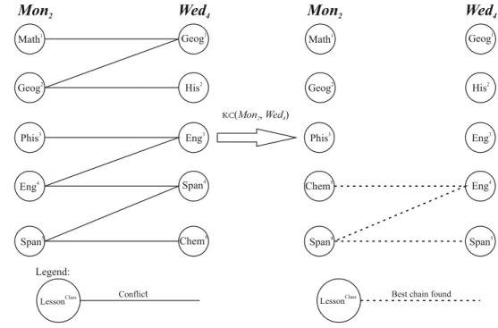
3.2.6 Kempe move (km)
Fig. 3 Example of event block swap (Fonseca et al. 2014)
Fig. 4 Example of resource swap (Fonseca et al. 2014)
Fig. 5 Example of resource move (Fonseca et al. 2014)
in the objective function assuming the exchange of timeslots between the events in the pair (n1,n2). Afterward, the method looks for the path with the lowest cost in the conflict graph and it makes the exchange of timeslots in the chain. This procedure is similar to that proposed by Tuga et al. (2007). Figure6presents an example of this move.
3.2.7 Move selection
The move k in N(s) is randomly selected in order to generate a neighbor. If the instance requires the assign-ment of resources (i.e., has at least oneAssign Resource constraint), the moves are chosen based on the following probabilities:es = 0.20, em = 0.38,ebs = 0.10,rs = 0.20,rm=0.10, andkm=0.02. Otherwise, the movesrs andrmare not used and the probabilities becomees=0.40, em=0.38,ebs=0.20, andkm=0.02. These values were adjusted based on empirical observation.
3.3 Late acceptance hill-climbing
The LAHC metaheuristic was proposed byBurke and Bykov (2008). This algorithm is an adaptation of the classical Hill-Climbing method. It relies on comparing a new candidate solution with the lastlth solution considered in the past, in order to accept or to reject it. Note that the candidate solution may be accepted even if it is worse than the current solution, since it is compared to the solution ofliterations before.
Fig. 6 Example of kempe move (Fonseca et al. 2014)
At each iterationi, a candidate solutions′is generated. The
candidate solution is accepted if its cost is less than or equal to the cost stored on thei modlposition ofp. Moreover, if this solution is better than the best solutions∗found so far,
a new incumbent solution is stored. Afterward, the position v = i modl of p is updated:pv ← f(s′). This process repeats until a stopping condition is met.
The implementation of the LAHC is illustrated in Algo-rithm 1. Note that timeout was adopted as the stopping condition for the algorithm. This decision is discussed in Sect.4. Some successful examples of application of LAHC can be found inAbuhamdah (2010),Özcan et al. (2009), Verstichel and Vanden Berghe(2009).
Algorithm 1: Developed implementation of LAHC
Input: Initial solutionsand parameterl.
Output: Best solutions∗found.
pk← f(s)∀k∈{0, ...,l- 1};
1
s∗←s;
2
i←0;
3
whileelapsed T i me<ti meoutdo 4
Generate a random neighbors′ ∈N(s);
5
v←imodl;
6
if f(s′)≤pvthen 7
s←s′;
8
if f(s) < f(s∗)then 9
s∗←s;
10
pv← f(s); 11
i←i+1;
12
returns∗;
13
Since it is relatively recent, variations of the LAHC meta-heuristic were not extensively explored yet. Therefore, the combination of LAHC with other methods and strategies is an open field for experimentation (Burke and Bykov 2012). In this paper we propose and evaluate computationally two LAHC variants, one of which is a hybrid version including SA.
3.3.1 Stagnation-free LAHC
In late stages of the LAHC execution, it is often very hard to improve the current solution. The algorithm can lead to a list with alll positions occupied with the same cost value, even for large values ofl. This behavior can make the LAHC incapable of escaping from local minima, since worse solu-tions are never accepted. A new variation of the LAHC, the so-called Stagnation-Free LAHC or simply sf-LAHC, is pro-posed in this paper in order to handle such situations.
Algorithm 2: sf-LAHC
Input: Initial solutionsand parameterslandmult.
Output: Best solutions∗found.
n←l×mult;
1
pk←p
′
k← f(s)∀k∈{0, ...,l- 1};
2
s∗←s; 3
i←0;
4
whileelapsed T i me<ti meoutdo 5
Generate a random neighbors′ ∈N(s);
6
v←imodl;
7
if f(s′)≤pvthen 8
s←s′;
9
if f(s) < f(s∗)then 10
s∗←s; 11
p′←p; 12
i←0;
13
pv← f(s); 14
i←i+1;
15
ifi=nthen 16
p←p′; 17
i←0;
18
returns∗;
19
3.3.2 Simulated annealing—LAHC
Proposed byKirkpatrick et al.(1983), the metaheuristic SA is a probabilistic method based on an analogy to thermo-dynamics, simulating the cooling of a set of heated atoms. This technique starts its search from any initial solution. The main procedure consists of a loop that randomly generates, at each iteration, one neighbors′ of the current solutions.
Movements are probabilistically selected considering a tem-peratureT and the cost variation obtained with the move, .
This algorithm was part of the solvers in all ITC winners (Fonseca et al. 2012;Kostuch 2005;Muller 2009). It also achieved good results in this model of the problem, espe-cially for larger instances. Therefore, it was evaluated in a hybrid approach with the LAHC algorithm. Since SA per-formance is not strongly affected by the fitness of the initial solution, it has been considered a mixed algorithm, with the SA algorithm being executed in the initial solution, gener-ating as∗solution, and the LAHC method being executed
further, to polish this solution, generating a final solution s∗∗. A combination of SA and sf-LAHC variant of LAHC was also tested. A mixed approach with as-LAHC was not presented because it achieved poor results.
The implementation of SA which is used in this work is described in Algorithm 3. Parameters were set as α = 0.97, T0 = 1, and SAmax = 10,000. The method select Movement()chooses a move according to the neigh-borhood probabilities previously defined.
Algorithm 3: Developed implementation of SA
Input:f(.),N(.), α,SAmax,T0,s,ti meout Output: Best solutions∗found.
s∗←s;I t er T←0;T ←T
0;r eheat s←0;
1
whileelapsed T i me<ti meoutdo 2
whileI t er T <SAmaxdo 3
I t er T←I t er T+1;
4
k←select Movement();
5
Generate a random neighbors′∈Nk(s);
6
Δ= f(s′)−f(s));
7
ifΔ <0then 8
s←s′;
9
if f(s′) < f(s∗)then s∗←s′
;
10
else 11
Takex∈ [0,1];
12
ifx<e−/Tthen s←s′
;
13
T←α×T;
14
I t er T←0;
15
returns∗; 16
4 Computational experiments
All experiments were executed on an Intel ® i5 2.4 GHz computer, 4 GB of RAM, under an Ubuntu 11.10 operating system. The software was coded in C++ and compiled with GCC 4.6.1. The obtained results were validated by a HSE-val HSE-validator.2The stopping criterion was 1,500 s timeout, adjusted according to the ITC2011 provided benchmark.
The results are expressed by the pairx/y, wherexstands for the feasibility measure and y for the quality measure. The proposed solver, along with solutions and reports, can be found at GOAL-UFOP website.3The interested reader is invited to validate the results.
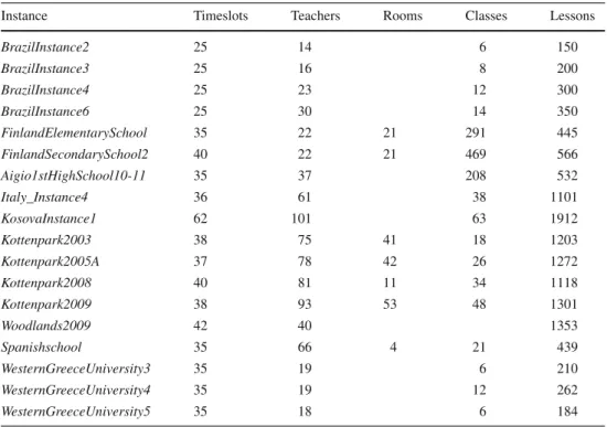
4.1 Dataset characterization
The set of instances available from ITC2011 (Post et al. 2014) is composed of problems from many countries, ranging from small to large and challenging instances. The main features of the considered instances are presented in Table1.
4.2 Parameter setting
One of the key advantages of LAHC is the small number of parameters to be set. Actually, the algorithm has only one parameter, which is the lengthlofpvector. As mentioned by Burke and Bykov(2008), higher values oflmake the search not only more suitable to find better results but also imply a higher processing time. On the other hand, low values of
2 http://sydney.edu.au/engineering/it/~jeff/hseval.cgi.
Table 1 Features of considered
instances from ITC2011 Instance Timeslots Teachers Rooms Classes Lessons
BrazilInstance2 25 14 6 150
BrazilInstance3 25 16 8 200
BrazilInstance4 25 23 12 300
BrazilInstance6 25 30 14 350
FinlandElementarySchool 35 22 21 291 445
FinlandSecondarySchool2 40 22 21 469 566
Aigio1stHighSchool10-11 35 37 208 532
Italy_Instance4 36 61 38 1101
KosovaInstance1 62 101 63 1912
Kottenpark2003 38 75 41 18 1203
Kottenpark2005A 37 78 42 26 1272
Kottenpark2008 40 81 11 34 1118
Kottenpark2009 38 93 53 48 1301
Woodlands2009 42 40 1353
Spanishschool 35 66 4 21 439
WesternGreeceUniversity3 35 19 6 210
WesternGreeceUniversity4 35 19 12 262
WesternGreeceUniversity5 35 18 6 184
l make the search faster but it can lead to poor results. For instance, if one considersl=1, the method performs exactly like the classical Hill-Climbing method.
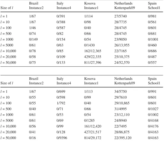
In this sense, experiments considering many values ofl: l = {1, 10, 100, 500, 1000, 5000, 10,000, 20,000, 50,000} have been executed. The instancesBrazilInstance2, ItalyIn-tance4,SpainSchool,KosovaInstance, and NetherlandsKot-tenpark2009have been chosen to determinate which value has the better average performance. These instances were chosen since they have different sizes and features. Tables2 and3present the results obtained under the considered con-figurations.
The poor performance observed forl =1 was expected, since the algorithms become identical to the original Hill-Climbing method. In general, it is possible to detect two different behaviors:
– for small instances, higherl values imply better perfor-mance, since the algorithm capacity of escaping from local optima increases. This can be seen for instance BrazilInstance2in Table3.
– for large instances, the performance of the method increases withl, but after some point it starts to decrease because the algorithm does not reach convergence before timeout in these cases. The instance KosovaInstance1, whose convergence curves are shown in Fig. 7, is an example of such a case. From this figure, it is possible to note that both, excessively high or excessively low values ofllead to bad results.
Based on the overall performances of the methods, we fixedl = 500 to perform the remaining experiments. This size has been chosen because it has shown to be a good com-promise between small and large instances.
4.3 Obtained results
Table4presents the results obtained with the LAHC method and its variants. The results obtained with the KHE engine (initial solution), the ITC2011 winner approach (SA-ILS), and the stand alone SA are also presented for comparison. The results presented are average values of five runs, with random seeds. The value of “Average ranking” was calcu-lated following the ITC2011 rules: each solution method was ranked between 1 and 5 on each instance (1 being the best and 5 being the worst), and the average of these ranks was taken. The best results are highlighted in bold.
Table 2 Experiments considering several values of parameterlon the original LAHC
Brazil Italy Kosova Netherlands Spain
Size ofl Instance2 Instance4 Instance1 Kottenpark09 School1
l= 1 1/67 0/391 1/114 27/5740 0/981
l= 10 1/67 0/388 0/98 28/7735 0/561
l= 100 1/46 0/587 0/40 28/4745 0/601
l= 500 0/74 0/82 0/66 28/4745 0/681
l= 1000 0/149 0/154 0/54 23/9050 0/1001
l= 5000 0/61 0/63 0/1430 26/13,955 0/460
l= 10,000 0/78 0/85 162/12,365 22/7165 0/686
l= 20,000 0/58 0/109 429/22,335 25/10,375 0/487
l= 50,000 0/75 0/133 811/27,396 24/52,570 0/557
Table 3 Experiments considering several values of parameterlon sf-LAHC
Brazil Italy Kosova Netherlands Spain
Size ofl Instance2 Instance4 Instance1 Kottenpark09 School1
l= 1 1/67 0/699 1/113 34/5750 0/991
l= 10 0/55 0/598 0/99 29/7610 0/601
l= 100 0/55 1/792 0/40 29/10,865 0/601
l= 500 0/40 0/71 0/66 31/4995 0/1027
l= 1000 0/61 0/53 0/54 23/12,110 0/1002
l= 5000 0/61 0/69 0/1285 24/8940 0/4168
l= 10,000 0/56 0/99 161/12,420 22/7495 0/4176
l= 20,000 0/41 0/128 427/21,517 28/86,875 0/4163
l= 50,000 0/16 0/9396 814/29,172 22/395,120 0/4163
Fig. 7 Behavior of LAHC regarding thelparameter to KosovaInstance1
0 0.2 0.4 0.6 0.8 1
0 500 1000 1500 2000 2500 3000 3500 4000 4500
average gap (%)
seconds KosovaInstance1
l=1 l=10 l=100 l=500 l=1000 l=5000 l=10000 l=20000 l=50000
4.4 Discussion of results
In some instances, even the production of feasible solutions is complicated, specially when most constraints are set as hard ones. The LAHC method and its variants were able to find 12 feasible solutions out of the 18 instances in the considered dataset, one more than the ITC2011 winner. In Table4, it
is possible to see that the LAHC algorithm and its variants outperformed the SA-ILS solver.
J
S
ched
(2016)
19:453–465
Table 4 Comparison between LAHC-based approaches and SA based methods
Instance KHE SA-ILS SA LAHC sf-LAHC SA-LAHC SA-sf-LAHC
BrazilInstance2 4/90 1.0/63.9 0.0/107.6 0.0/78.6 0.0/52.8 0.0/102.4 0.0/78.0
BrazilInstance3 3/240 0.0/127.8 0.0/170.6 0.0/145.6 0.0/137.0 0.0/174.0 0.0/160.2
BrazilInstance4 39/144 17.2/99.6 2.0/167.4 8.2/121.4 6.0/112.8 2.4/165.6 2.4/164.2
BrazilInstance6 11/291 4.0/223.5 0.0/332.2 1.4/204.8 0.6/166.4 0.0/252.6 0.0/221.0
FinlandElementarySchool 9/30 0.0/4.0 0.0/10.0 0.0/3.8 0.0/3.6 0.0/3.8 0.0/3.8
FinlandSecondarySchool2 2/1821 0.0/0.4 0.0/1036.4 0.0/0.4 0.0/0.2 0.0/0.2 0.0/0.4
Aigio1stHighSchool10-11 14/757 0.0/15.3 0.0/397.4 0.8/11.4 0.8/11.4 0.0/17.8 0.0/20.8
Italy_Instance4 39/21238 0.0/658.4 0.0/13979.0 0.0/224.8 0.0/199.4 0.0/366.4 0.0/302.2
KosovaInstance1 1333/566 14.0/6934.4 3.0/5837.8 14.2/1504.8 0.0/137.0 4.6/5238.6 6.3/6383.8
Kottenpark2003 3/78440 0.6/90195.8 0.4/90052.4 1.6/9711.0 1.6/9136.8 0.0/69608.2 0.4/89132.2
Kottenpark2005A 35/23677 33.9/27480.4 30.0/33967.0 33.0/18671.0 32.8/18891.8 30.2/33310.4 30.2/33169.6
Kottenpark2008 63/140083 25.7/31403.7 10.0/138993.8 15.2/23855.0 14.4/23067.2 10.8/57476.6 10.8/59939.2
Kottenpark2009 55/211095 36.6/154998.5 24.6/432784.0 28.0/9192.0 28.8/8363.0 25.4/112948.0 25.8/112335.0
Woodlands2009 19/0 2.0/15.8 2.0/223.8 2.0/13.2 2.0/12.0 2.0/12.4 2.0/12.0
Spanish school 1/4103 0.0/865.2 0.0/7077.6 0.0/846.0 0.0/920.4 0.0/998.2 0.0/856.8
WesternGreeceUniversity3 0/30 0.0/5.6 0.0/28.4 0.0/5.0 0.0/5.0 0.0/5.4 0.0/5.2
WesternGreeceUniversity4 0/41 0.0/7.4 0.0/39.4 0.0/9.2 0.0/6.8 0.0/7.6 0.0/6.6
WesternGreeceUniversity5 17/44 0.0/0.0 0.0/56.0 0.0/0.0 0.0/0.0 0.0/0.0 0.0/0.0
ched
(2016)
19:453–465
463
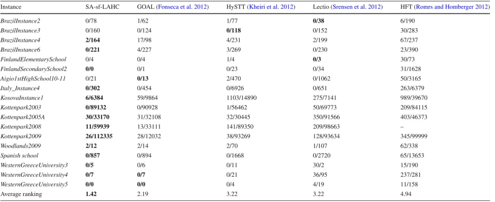
Table 5 Comparison of results between SA-sf-LAHC and ITC2011 finalists
Instance SA-sf-LAHC GOAL (Fonseca et al. 2012) HySTT (Kheiri et al. 2012) Lectio (Srensen et al. 2012) HFT (Romrs and Homberger 2012)
BrazilInstance2 0/78 1/62 1/77 0/38 6/190
BrazilInstance3 0/160 0/124 0/118 0/152 30/283
BrazilInstance4 2/164 17/98 4/231 2/199 67/237
BrazilInstance6 0/221 4/227 3/269 0/230 23/390
FinlandElementarySchool 0/4 0/4 1/4 0/3 30/73
FinlandSecondarySchool2 0/0 0/1 0/23 0/34 31/1628
Aigio1stHighSchool10-11 0/21 0/13 2/470 0/1062 50/3165
Italy_Instance4 0/302 0/454 0/6926 0/651 263/6379
KosovaInstance1 6/6384 59/9864 1103/14890 275/7141 989/39670
Kottenpark2003 0/89132 0/90928 1/56462 50/69773 209/84115
Kottenpark2005A 30/33170 31/32108 32/30445 350/91566 403/46373
Kottenpark2008 11/59939 13/33111 141/89350 209/98663 –
Kottenpark2009 26/112335 28/12032 38/93269 128/93634 345/99999
Woodlands2009 2/12 2/14 2/70 1/107 62/338
Spanish school 0/857 0/894 0/1668 0/2720 65/13653
WesternGreeceUniversity3 0/5 0/6 0/11 30/2 15/190
WesternGreeceUniversity4 0/7 0/7 0/21 36/95 237/281
WesternGreeceUniversity5 0/0 0/0 0/4 4/19 11/158
Average ranking 1.42 2.19 3.22 3.22 4.94
better than the SA. This is an interesting result, since LAHC is a new metaheuristic and it is still open for improvements. In addition, the SA is known as a good algorithm for dealing with scheduling problems, which makes the observed result a good achievement.
The Stagnation-Free version of LAHC obtained good results, outperforming its original version in several instances. This could be noted specially in small instances, in which sf-LAHC can keep some improvement until the timeout is reached instead of the original LAHC, which probably got stuck at a local optima. Finally, it is important to highlight the remarkable performance observed for the combination of LAHC and SA proposed in this work (SA-sf-LAHC). This heuristic obtained the best results and, compared to the final-ist results (see Table5), it is possible to conclude that it would win the competition by a large margin: it reached the best result in 14 out of 18 instances, leading to an overall rank-ing of 1.42. A two-tail Welchs T-test, comparrank-ing GOAL and LAHC rankings, reinforced the assumption of SA-sf-LAHC superiority: it has obtained a p-value of 8.0254e−06, which widely supports the rejection of the null hypothesis (equivalent algorithms) under the confidence level of 95 %.
5 Concluding remarks
This work presented an application of the Late Acceptance Hill-Climbing algorithm to the HSTP model proposed in the ITC2011. In addition, some variants of the LAHC method were proposed and evaluated computationally.
The LAHC algorithm obtained good results. It was able to outperform the stand-alone SA approach and the ITC2011 winner approach, a SA-ILS method. The LAHC variants proposed in this paper also reached promising results. The Stagnation-Free LAHC (sf-LAHC) was able to outperform its original version. The combinations of LAHC and sf-LAHC with SA were tested, and the mixed SA-sf-sf-LAHC algorithm achieved the best results to this problem up to now. One great feature of LAHC is its simplicity: it is very easy to implement and it relies only on one parameter to be tuned.
Some possible future extensions of this work are (i) to develop and to evaluate other variations of LAHC as sug-gested byBurke and Bykov(2008); (ii) to implement and to evaluate other neighborhood moves; and (iii) to develop a graphical user interface to allow the use of the solver by schools and universities.
References
Abuhamdah, A. (2010). Experimental result of late acceptance random-ized descent algorithm for solving course timetabling problems.
IJCSNS-International Journal of Computer Science and Network Security,10(1), 192–200.
Burke, E. K., & Bykov, Y. (2008). A late acceptance strategy in hill-climbing for exam timetabling problems. InPATAT’08 pro-ceedings of the 7th international conference on the practice and theory of automated timetabling.
Burke, E. K., & Bykov, Y. (2012). The late acceptance hill-climbing heuristic. Technical Report CSM-192, Department of Computing Science and Mathematics, University of Stirling.
de Haan, P., Landman, R., Post, G., & Ruizenaar, H. (2007). A case study for timetabling in a dutch secondary school. InLecture notes in computer science: VI. Practice and theory of automated timetabling(Vol. 3867, pp. 267–279). Berlin: Springer.
Dorneles, Á. P., de Araújo, O. C., & Buriol, L. S. (2014). A fix-and-optimize heuristic for the high school timetabling problem. Computers & Operations Research,52, 29–38.
Fonseca, G., Santos, H., Toffolo, T., Brito, S., & Souza, M. (2012). A SA-ILS approach for the high school timetabling problem. In PATAT’12 proceedings of the 9th international conference on the practice and theory of automated timetabling.
Fonseca, G. H. G., Santos, H. G., Toffolo, T. A. M., Brito, S. S., & Souza, M. J. F. (2014). GOAL solver: A hybrid local search based solver for high school timetabling.Annals of Operations Research, 1–21. doi:10.1007/s10479-014-1685-4.
Garey, M. R., & Jonhson, D. S. (1979).Computers and intractability: A guide to the theory of NP-completeness. San Francisco, CA: Freeman.
IDSIA (2012). International Timetabling Competition 2002 (2012). Retrieved December, 2012 from http://www.idsia.ch/Files/ ttcomp2002/.
Kheiri, A., Ozcan, E., & Parkes, A. J. (2012). Hysst: Hyper-heuristic search strategies and timetabling. InProceedings of the ninth international conference on the practice and theory of automated timetabling (PATAT 2012)(pp. 497–499).
Kingston, J. (2014). KHE14 an algorithm for high school timetabling. In10th international conference on the practice and theory of automated timetabling(pp. 26–29).
Kingston, J. H. (2005) A tiling algorithm for high school timetabling. InLecture notes in computer science: V. Practice and theory of automated timetabling(Vol. 3616, pp. 208–225). Berlin: Springer. Kingston, J. H. (2012). A software library for school timetabling (2012). Retrieved May, 2012, from http://sydney.edu.au/engineering/it/ ~jeff/khe/.
Kingston, J. H. (2012). A software library for school timetabling (2012). Retrieved December 2012, from http://sydney.edu.au/ engineering/it/~jeff/khe/.
Kirkpatrick, S., Gelatt, C. D., & Vecchi, M. P. (1983). Optimization by simulated annealing.Science,220, 671–680.
Kostuch, P. (2005). The university course timetabling problem with a three-phase approach. In Proceedings of the 5th inter-national conference on practice and theory of automated timetabling, PATAT’04(pp. 109–125). Berlin: Springer. doi:10. 1007/11593577_7.
Kristiansen, S., Srensen, M., Stidsen, T. (2014). Integer programming for the generalized high school timetabling problem.Journal of Scheduling, 1–16. doi:10.1007/s10951-014-0405-x.
McCollum, B. (2012). International timetabling competition 2007. Retrieved December, 2012 from http://www.cs.qub.ac.uk/ itc2007/.
Moura, A. V., & Scaraficci, R. A. (2010). A grasp strategy for a more constrained school timetabling problem.International Journal of Operational Research,7(2), 152–170.
Nurmi, K., & Kyngas, J. (2007). A framework for school timetabling problem. InProceedings of the 3rd multidisciplinary international scheduling conference: theory and applications, Paris(pp. 386– 393).
Özcan, E., Bykov, Y., Birben, M., & Burke, E. K. (2009). Examination timetabling using late acceptance hyper-heuristics. InProceedings of the eleventh conference on congress on evolutionary computa-tion, CEC’09(pp. 997–1004). IEEE Press, Piscataway, NJhttp:// dl.acm.org/citation.cfm?id=1689599.1689731.
Pillay, N. (2013) A survey of school timetabling research.Annals of Operations Research, 1–33.
Post, G., Kingston, J., Ahmadi, S., Daskalaki, S., Gogos, C., Kyngas, J., et al. (2014). XHSTT: An XML archive for high school timetabling problems in different countries.Annals of Operations Research, 218(1), 295–301.
Romrs, J., & Homberger, J. (2012). An evolutionary algorithm for high school timetabling. InPATAT’12 proceedings of the 9th inter-national conference on the practice and theory of automated timetabling.
Santos, H. G., Uchoa, E., Ochi, L. S., & Maculan, N. (2012). Strong bounds with cut and column generation for class-teacher timetabling.Annals OR,194(1), 399–412.
Srensen, M., Kristiansen, S., & Stidsen, T. (2012). International timetabling competition 2011: An adaptive large neighborhood search algorithm (pp. 489–492).
Tuga, M., Berretta, R., & Mendes, A. (2007) A hybrid simulated anneal-ing with kempe chain neighborhood for the university timetablanneal-ing problem. In6th IEEE/ACIS international conference on computer and information science, 2007. ICIS 2007, IEEE (pp. 400–405). Valourix, C., & Housos, E. (2003). Constraint programming approach
for school timetabling. InComputers & Operations Research(pp. 1555–1572).
Verstichel, J., & Vanden Berghe, G. (2009). A late acceptance algorithm for the lock scheduling problem. In S. Voss, J. Pahl, & S. Schwarze (Eds.),Logistik management(pp. 457–478). Dordrecht: Springer. Wright, M. (1996). School timetabling using heuristic search.Journal