http://www.ntmsci.com
An approach to numerical solutions of system of
high-order linear differential-difference equations with
variable coefficients and error estimation based on
residual function
Nebiye Korkmaz1and Mehmet Sezer2
1Department of Secondary Science and Mathematics Education, Faculty of Education, Mugla Sitki Kocman University, 48000 Mugla, Turkey
2Department of Mathematics, Celal Bayar University, 45140, Manisa,Turkey
Received: 27 September 2014, Revised: 19 October 2014, Accepted: 14 Novamber 2014 Published online: 6 December 2014
Abstract: In this study a method is presented which aims to make an approach by using Bernstein polynomials to solutions of systems of high order linear differential-difference equations with variable coefficients given under mixed conditions. The method converts a given system of differential-difference equations and the conditions belonging to this system to equations that can be expressed by matrices by using the collacation points and provides to find the unknown coefficients of approximate solutions sought in terms of Bernstein polynomials. Different examples are presented with the purpose to show the applicability and validity of the method. Absolute error values between exact and approximate solutions are computed. The estimated values of absolute errors are computed by using the residual function and these estimated errors are compared with absolute errors. For all numerical computations of this study the computer algebraic system Maple 15 is used.
1 Introduction
Differential-difference equations and systems of these class of equations are used to model various science and engineering problems. Since solving systems of differential-difference equations analytically is hard, several numerical methods are improved to solve these systems. We can give examples of some particular methods used for solving these systems such as variational iteration method [16], differential transformation method [1], Adomian decomposition method [9], differential transform method [17], linearizability criteria [10], decomposition method [4], homotopy analysis method [21], homotopy perturbation method [12], Bessel matrix method [20], Taylor collacation Method [8].
In this study, modifying and developing methods in [2,8,13,20] and using matrix relations between Bernstein polynomials and their derivatives, we present an approach to numerical solutions of systems of linear high-order differential-difference equations with variable coefficients in the form
m
∑
r=0k
∑
i=1Prj,i(x)y(ir)(λx+β) =fj(x), j=1,2,· · ·,k (1)
given together with mixed conditions defined as follows
m−1
∑
j=1anr,j(x)yn(j)(a) +bnr,j(x)y
(j)
n (b) +cnr,j(x)y
(j)
n (c) =λn,r, (2)
a≤c≤b, r=0,1,2,· · ·,m−1, n=1,2,· · ·,k
whereyj represents an unknown function, Pj,i represent the known functions and fj are defined on the closed interval
Our main purpose is to find the approximate solutions of system given with (1) expressed in the following truncated Bernstein series form:
yi(x) = N
∑
n=0yn,iBn,N(x), a≤x≤b, i=1,2,· · ·,k (3)
whereyn,i,(i=1,2,· · ·,k,n=0,1,· · ·,N)are the unknowns coefficients to be determined andNis any positive integer
such thatN≥m.
2 Bernstein Polynomials
General form of thenth degree Bernstein polynomials are defined by [3] as follows:
Bi,N(x) = (
N i )
xi(R−x)N−i
RN , i=0,1,· · ·,N
where whereRis the maximum range of the interval[0,R]over which the polynomials are defined to form a complete basis. In [3] it is mentioned that there aren+1nth degree polynomials andBi,N(x) =0 fori<0 andi>N.
Bernstein polynomials can be generated by a recursive formula over an interval[0,R], so that theithNth degree Bernstein polynomial can be written as
Bi,N(x) = R−x
R Bi,N−1(x) + x
RBi−1,N−1(x)
As also it is mentioned in [3], any polynomial of degreencan be expanded in terms of a linear combination of the basis functions:
P(x) =
i=0
∑
NCiBi,N(x), N≥1.
3 Fundamental Matrix Relations
We can convert the Bernstein series solutionsyi(x)given with (3) and their derivativesy(ir)(x)in to matrix forms
yi(x) =BN(x)Ai, i=1,2,· · ·,k (4)
and
y(ir)(x) =B(Nr)(x)Ai i=1,2,· · ·,k (5)
where
BN(x) = [
B0,N(x)B1,N(x)· · · BN,N(x)],Ai= [
y0,iy1,i · · · yN,i]T. BN(x)can be represented as
BN(x) =X(x).B (6)
where
X(x) =[1x x2· · · xN]T, B=
b00 b01 · · · b0N b10 b11 · · · b1N
..
. ... . .. ...
bN0bN1· · · bNN
andbi j=
{(−1)i−j Ri
(N j
)(N−j i−j )
, i≥j
0, i<j.
For the matrix representations of the derivatives of approximate solutions we need the relation betweenX(x)and its derivativeX(1)(x)which can be clearly seen as
X(1)(x) =X(x)D (7)
where
D=
0 1 0 0· · · 0 0 0 2 0· · · 0 0 0 0 3· · · 0
..
. ... ... ... . .. ... 0 0 0 0· · · N
We obtain all the derivativesX(r)(x)in terms ofX(x)with the help of (7) by following calculations below:
X(2)(x) =X(1)(x)D=X(x)D2
.. .
X(r)(x) =X(r−1)(x)D=X(x)Dr (8)
We reach similar relations betweenX(λx+β)and its derivativesX(r)(λx+β)by using (8) given as follows:
X(λx+β) = [1 λx+β (λx+β)2· · ·(λx+β)N] =X(x)C(λ,β) (9)
X(1)(λx+β) =X(λx+β)D=X(x)C(λ,β)D
X(2)(λx+β) =X(λx+β)D2=X(x)C(λ,β)D2
.. .
X(r)(λx+β) =X(λx+β)Dr=X(x)C(λ,β)Dr (10)
where forλ̸=0 andβ̸=0C(λ,β)is defined as
C(λ,β) =
(0 0
)
λ0β0(1 0
)
λ0β1· · · (N
0
)
λ0βN
0 (11)λ1β0· · · (N
1
)
λ1βN−1
..
. ... . .. ...
0 0 · · · (NN)λNβ0
and for the valuesλ =1 andβ =0 defined as
C(λ,0) =
λ0 0 · · · 0
0 λ1· · · 0
..
. ... . .. ... 0 0 · · ·λN
Substituting (6) into (4) we get the matrix representation ofyiin (4) as
yi(x) =X(x)BAi, i=1,2,· · ·,k (11)
Differentiating (11) consecutively with respect toxand using (8) we get the matrix expression ofy(ir)in (5) as follows:
y(ir)(x) =X(x)DrBAi, i=1,2,· · ·,k (12)
By means of (9), (10), (11) and (12) we obtain the matrix relations
y(ir)(λx+β) =X(x)C(λ,β)DrBAi, i=1,2,· · ·,k (13)
Let us define the matrices
y(r)(λx+β) =
y(1r)(λx+β)
y(2r)(λx+β)
.. .
y(kr)(λx+β)
r=0,1,· · ·,m (14)
which can be expressed by means of the relations given with (12) as
y(r)(λx+β) =X∗(x)C∗(λ,β)DerBAe , r=0,1,· · ·,m (15)
X∗(x) =
X(x) 0 · · · 0 0 X(x)· · · 0
..
. ... . .. ... 0 0 · · · X(x)
,Der=
Dr 0 · · · 0 0 Dr · · · 0
..
. ... . .. ... 0 0 · · · Dr
, e B=
B0 · · · 0 0 B· · · 0
.. . ... . .. ... 0 0· · · B
,C∗(λ,β) =
C(λ,β) 0 · · · 0 0 C(λ,β)· · · 0
..
. ... . .. ...
0 0 · · ·C(λ,β)
andA= [
A1A2· · · Ak]T.
4 Method of Solution
We can express the system given with (1) in the matrix form
m
∑
r=0Pr(x)y(r)(λx+β) =f(x) (16)
wherey(r)(λx+β)is as the form (14), f(x) =[f1(x) f2(x)· · · fk(x) ]T
andPr(x) =
P1r,1(x)P1r,2(x)· · · P1r,k(x)
P2r,1(x)P2r,2(x)· · · P2r,k(x)
..
. ... . .. ...
Pkr,1(x)Pkr,2(x)· · · Pkr,k(x)
.By
substituting the node points{xi|0=x0<x1<· · ·<xN=R,i=0,1,· · ·,N}into the matrix equation (16) we obtain the
system of fundamental matrix equation as
m
∑
r=0Pr(x)Y(r)=F (17)
wherePr=
Pr(x0) 0 · · · 0
0 Pr(x1)· · · 0
..
. ... . .. ...
0 0 · · · Pr(xN)
, Y(r)=
y(r)(λx0+β)
y(r)(λx1+β)
.. .
y(r)(λxN+β) T
andf(x) =[f(x0) f(x1)· · · f(xN)]T.
Using the node points and (15) we can rewriteY(r)in the matrix form
Y(r)=XC∗(λ,β)DerBAe , r=0,1,· · ·,m (18)
where
X=[X∗(x0)X∗(x1)· · · X∗(xN)]T.
Substituting (18) into expression (17) we have the fundamental matrix equation
{ m
∑
r=0PrXC∗(λ,β)DerBe }
A=F (19)
The fundamental matrix relation (19) corresponding to equation system (1) can be expressed in the following form
WA=For[W;F] (20)
where
W = [Wp,q] = m
∑
r=0PrXC∗(λ,β)DerBe, p,q=1,2,· · ·,k(N+1) (21)
which is a linear system of k(N +1) algebraic equations in k(N +1) unknown Bernstein coefficients
following a similar way used for the system (1). Writing the conditions in (2) for eachnwe have the following equations
m−1
∑
j=0a1r,jy(1j)(a) +b1r,jy1(j)(b) +c1r,jy1(j)(c) =λ1,r
m−1
∑
j=0a2r,jy(2j)(a) +b2r,jy2(j)(b) +c2r,jy2(j)(c) =λ2,r
.. .
m−1
∑
j=0akr,jy(kj)(a) +bkr,jyk(j)(b) +ckr,jyk(j)(c) =λk,r
which we can also express as
m−1
∑
j=0A0,jy(j)(a) +B0,jy(j)(b) +C0,jy(j)(c) =λ0
m−1
∑
j=0A1,jy(j)(a) +B1,jy(j)(b) +C1,jy(j)(c) =λ1
.. .
m−1
∑
j=0Am−1,jy(j)(a) +Bm−1,jy(j)(b) +Cm−1,jy(j)(c) =λm−1
where
Ar,j=
a1r,j 0 · · · 0 0 a2r,j· · · 0
..
. ... . .. ... 0 0 · · · akr,j
,Br,j=
b1r,j 0 · · · 0 0 b2r,j · · · 0
..
. ... . .. ... 0 0 · · ·bkr,j
,
Cr,j=
c1r,j 0 · · · 0 0 c2r,j· · · 0
..
. ... . .. ... 0 0 · · · ck r,j
andλr= [
λ1,r λ2,r· · · λk,r ]T
,
forr=0,1,· · ·,m−1 or briefly
m−1
∑
j=0Ajy(j)(a) +Bjy(j)(b) +Cjy(j)(c) =λ (22)
where
Aj= [
A0,j A1,j · · ·Am−1,j ]T
,Bj= [
B0,jB1,j· · · Bm−1,j ]T
,
Cj=[C0,jC1,j· · ·Cm−1,j]T andλ=[λ0λ1· · · λm−1]T.
By substitutingλ=1 andβ =0 in (14) and calculating this matrix at pointsa,bandc, we get the matrix representations ofyj(a),yj(b)andyj(c)in (22) as follows:
y(j)(a) =X∗(a)DejA
y(j)(b) =X∗(b)DejA
Substituting the matrices given in (23) in the equation (22) and simplifying the result we obtain the matrix representation of the conditions containing the coefficient matrixAas
λ=
m−1
∑
j=0[AjX∗(a) +BjX∗(b) +CjX∗(c)]DejA (24)
Defining the matrix
V =
m−1
∑
j=0[AjX∗(a) +BjX∗(b) +CjX∗(c)]Dej (25)
we can write the matrix form of the conditions given with (24) as
VA=λ (26)
Finally by replacing number ofmkrows of the matrixW andF with the rows of the matrixV andλ, respectively, we obtain the unknown coefficients of the approximate solutions of the system (1). Generally for simplicity we prefer to use the last rows of the matrices for replacement and in this we illustrate this replacement procedure as follows:
e
W A=Fe (27)
where
e W=
W1,1 W1,2 · · · W1,k(N+1)
W2,1 W2,2 · · · W2,k(N+1)
..
. ... ... ...
Wk(N−m+1),1Wk(N−m+1),2· · ·Wk(N−m+1),k(N+1) V1,1 V1,2 · · · V1,k(N+1)
V2,1 V2,2 · · · V2,k(N+1)
..
. ... ... ...
Vkm,1 Vkm,2 · · · Vkm,k(N+1)
andFe=[f1(x0)· · · fk(x0) f1(x1)· · · fk(xN−m)λ1,0· · · λ1,m−1λ2,0· · · λk,m−1
]T
. If the matrixW is singular, then the rows having the same factor or all zero are replaced. HenceAis obtained as
A= (We)−1Fe. (28)
5 Error Estimation Based on Residual Function
Researchers used the residual error estimation for residual correction [5,11], the error estimation of the Tau method for
integro-differential equations [14], error estimation of the Bessel collacation method for the multi-pantograph
equations [18], Laguerre matrix method for delay differential equations [19]. In this section we present an error
estimation based on residual function by modifying the error estimation studied in [5,11,14,18,19]. Let
ei,N(x) =yi(x)−yi,N(x),(i=1,· · ·,k)denote the error function of approximate solutionyi,Ntoyi, whereyiis one of the
exact solutions of the problem of equation system given with (1) and (2). Henceyi,N(x)satisfies the following problem
which can be obtained by substituting the approximate solutionyi,Ninto the problem given with (1) : m
∑
r=0k
∑
i=1Pjr,i(x)yi(,rN)(λx+β) = fj(x) +Rj,N(x), x∈[a,b], j=1,2,· · ·,k (29)
with the mixed conditions
m−1
∑
j=1arn,j(x)yn(,jN)(a) +bnr,j(x)yn(,jN)(b) +cnr,j(x)y(nj,N)(c) =λn,r, (30)
whereRj,N,(n=1,2,· · ·,k)denote the residual functions associated with the approximate solutionsyj,N. Subtracting (29)
and (30) from (1) and (2),respectively, the following error problem
m
∑
r=0k
∑
i=1Pjr,i(x)e(i,rN)(λx+β) =−Rj,N(x), x∈[a,b], j=1,2,· · ·,k (31)
with the mixed conditions
m−1
∑
j=1anr,j(x)e(n,jN)(a) +bnr,j(x)e(n,jN)(b) +cnr,j(x)e(nj,N)(c) =0, (32)
a≤c≤b, r=0,1,2,· · ·,m−1, n=1,2,· · ·,k
is obtained which is satisfied by the error functionsei,N,(i=1,2,· · ·,k). Solving this error problem with the same
method given in section4the approximationei,N,M to errorei,N is attained. The advantage of solving this error problem
is that the error of the approximate solution can be estimated without knowing the exact solution. In the next section we prefer to use examples whose exact solutions are known in order to compare the exact errors with the estimated errors.
6 Numerical Examples
Example 1.Consider the following linear differential-difference equation system and the conditions given by
−xy(11)(x+1) +2y1(x+1) +2y2(x+1) =x+7
2y2(x+1)−3y1(1)(x+1)−4y
(2)
1 (x+1) =0
y1(1/2) =3/4,y2(1/2) =11/2,y1(1) =0,y2(1) =7
where 0≤x≤1. ForN=3 the nodes arex0=0,x1=13,x2=23,x4=1. Fundamental matrix equation of the problem is
{P0XC∗(1,1)Be+P1XC∗(1,1)DeBe+P2XC∗(1,1)De2B}Ae =F
where
P0=
2 1 0 0 0 0 0 0 0 2 0 0 0 0 0 0 0 0 2 1 0 0 0 0 0 0 0 2 0 0 0 0 0 0 0 0 2 1 0 0 0 0 0 0 0 2 0 0 0 0 0 0 0 0 2 1 0 0 0 0 0 0 0 2
,P1=
0 0 0 0 0 0 0 0
−3 0 0 0 0 0 0 0
0 0−130 0 0 0 0
0 0−3 0 0 0 0 0
0 0 0 0−2
3 0 0 0
0 0 0 0−3 0 0 0
0 0 0 0 0 0−1 0
0 0 0 0 0 0−3 0
,
P2=
0 0 0 0 0 0 0 0
−4 0 0 0 0 0 0 0
0 0 0 0 0 0 0 0
0 0−4 0 0 0 0 0
0 0 0 0 0 0 0 0
0 0 0 0−4 0 0 0
0 0 0 0 0 0 0 0
0 0 0 0 0 0−4 0
,X=
1 0 0 0 0 0 0 0 0 0 0 0 1 0 0 0 1 13 19 271 0 0 0 0 0 0 0 0 1 13 19 271 1 23 49 278 0 0 0 0 0 0 0 0 1 23 49 278 1 1 1 1 0 0 0 0 0 0 0 0 1 1 1 1
e B=
1 0 0 0 0 0 0 0
−3 3 0 0 0 0 0 0
3 −6 3 0 0 0 0 0
−1 3 −3 1 0 0 0 0
0 0 0 0 1 0 0 0
0 0 0 0−3 3 0 0
0 0 0 0 3 −6 3 0
0 0 0 0−1 3 −3 1
,C∗(1,1) =
1 1 1 1 0 0 0 0 0 1 2 3 0 0 0 0 0 0 1 3 0 0 0 0 0 0 0 1 0 0 0 0 0 0 0 0 1 1 1 1 0 0 0 0 0 1 2 3 0 0 0 0 0 0 1 3 0 0 0 0 0 0 0 1 , e D=
0 1 0 0 0 0 0 0 0 0 2 0 0 0 0 0 0 0 0 3 0 0 0 0 0 0 0 0 0 0 0 0 0 0 0 0 0 1 0 0 0 0 0 0 0 0 2 0 0 0 0 0 0 0 0 3 0 0 0 0 0 0 0 0
,
,F=
7 0 22 3 0 23 3 0 23 3 0
,A=
[ A1
A2
] ,
A1=
y0,1
y1,1
y2,1
y3,1
,A2=
y0,2
y1,2
y2,2
y3,2
.
Using the above matrices we obtain the matrixW defined with (21) as
W=
0 0 0 2 0 0 0 1
0 −24 57 −33 0 0 0 2
1 27 −1 9 −8 9 80 27 −1 27 4 9 −16 9 64 27
9 −57 96 −48−2
27 8 9 − 32 9 128 27 8 27 − 8 9 − 10 9 100 27 − 8 27 20 9 − 50 9 125 27
20 −96 141 65 −1627 409 −1009 25027
1 −3 0 1 4 6 −12 8
33−141 192 −84 −2 12 −24 16
.
From (24), (25) and (26) matrix representation of the given conditions are obtained as
V= 1 8 3 8 3 8 1
8 0 0 0 0
0 0 0 0 18 38 38 18 0 0 −3 3 18 38 38 18
0 0 0 0 0 0 −3 3
,λ=
−3 4 11 2 0 7
,VA=λ.
By performing the row replacement we obtain the matricesWe andFein (27) as follows:
e W =
0 0 0 2 0 0 0 1
0 −24 57 −33 0 0 0 2
1 8 3 8 3 8 1
8 0 0 0 0
0 0 0 0 18 38 38 18
0 0 −3 3 18 38 38 18
0 0 0 0 0 0−3 3
,Fe=
7 0 22 3 −3 4 11 2 0 7 .
By using (28), the unknown coefficient matrixAis obtained as
A=[−1−1−2
3 0 4 5 6 7
]T .
Hence substituting appropriate coefficients in (4) we obtain the approximate solutions as
y1(x) =x2−1,y2(x) =3x+1.
Example 2.( [8], [17], [20]) Consider the following linear differential system and the condition given with:
y(11)(x) +y(21)(x) +y1(x) +y2(x) =1
y(21)(x)−2y1(x)−y2(x) =0
y1(0) =0,y2(0) =1
where 0≤x≤1. Exact solutions of this system arey1(x) =e−x−1 andy2(x) =2−e−x. For this example we can align
the basic values of the problem as k = 2,m = 1,λ = 1,β = 0,f1(x) = 1, f2(x) = 0,
P0
1,1=1,P10,2=1,P20,1=−2,P20,2=−1,P11,1=1,P11,2=1,P21,1=0,P21,2=1.Fundamental matrix equation of the problem
is
{P0XC∗(1,0)Be+P1XC∗(1,0)DeB}Ae =F
Following the method given in section4we obtain the approximate solutions fori=1,2 andN=6,8,10 as
y1,6(x) =−t+0.49999287763359t2−0.1665992415988t3+ (0.414094305449e−1)t4
−(0.78459973259e−2)t5+ (0.92305849257e−3)t6 ,
y2,6(x) =1+1.00000000000002t−0.4999928776345t2+0.1665992416052t3
−(0.414094305609e−1)t4+ (0.78459973420e−2)t5−(0.92305849852e−3)t6,
y1,8(x) =−t+0.49999998063417t2−0.1666663924244t3+ (0.416649836193e−1)t4
−(0.8327671049e−2)t5+ (0.13776655847e−2)t6−(0.1852302697e−3)t7
+ (0.16106411517e−4)t8 ,
y2,8(x) =1+t−0.4999999806306t2+0.1666663923794t3−(0.416649833725e−1)t4
+ (0.8327670334e−2)t5−(0.13776644215e−2)t6+ (0.1852292920e−3)t7
−(0.1610607624e−4)t8 ,
y1,10(x) =−t+0.4999999999679721464t2−0.166666666051952172t3
+ (0.41666661337852444e−1)t4−(0.833330671871991e−2)t5+ (0.138880521754404e−2)t6
−(0.1982411886115e−3)t7+ (0.245716339029e−4)t8−(0.2559545198236e−5)t9
+ (0.17652035850008e−6)t10 ,
y2,10(x) =1+t−0.499999999967972145t2+0.16666666605195216t3
−(0.4166666133785242e−1)t4+ (0.83333067187197e−2)t5−(0.13888052175437e−2)t6
+ (0.1982411886110e−3)t7−(0.24571633902642e−4)t8+ (0.25595451979e−5)t9
−(0.1765203584601e−6)t10 .
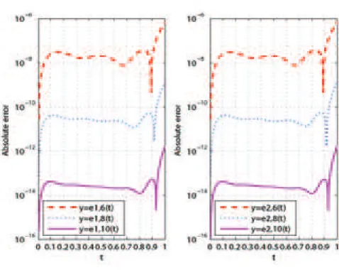
Comparison of absolute error values with the ones in [8], [17] and [20] are given in tables 1and 3. As seen from the tables we obtain better results rather than Transform method [17] and we obtain very similar results to Bessel Method [20] and Taylor method [8] results. The estimated errors for the error functionse1,6ande2,6are given in tables 2and 4from
which we can see that our estimations are very close to exact errors. In Figure1 graphs of the error functionse1,N and e2,Nfor the valuesN=6,8,10 are given. It is clearly seen from these graphs that errors are decreasing as the value ofN
Table 1:Numerical results of absolute error functione1,6of Example2
xi Transform Method [17] Bessel Method [20] Taylor Method [8] Present Method
0 0 0 0 0
0.2 1.5575e-002 2.8460e-008 2.845945e-008 2.845996e-008
0.4 5.1209e-002 1.7820e-008 1.782165e-008 1.781967e-008
0.6 1.0150e-001 1.2668e-008 1.267680e-008 1.266769e-008
0.8 1.6630e-001 3.3538e-008 3.356743e-008 3.353739e-008
1 2.3351e-001 6.8657e-007 6.865716e-007 6.86574918e-007
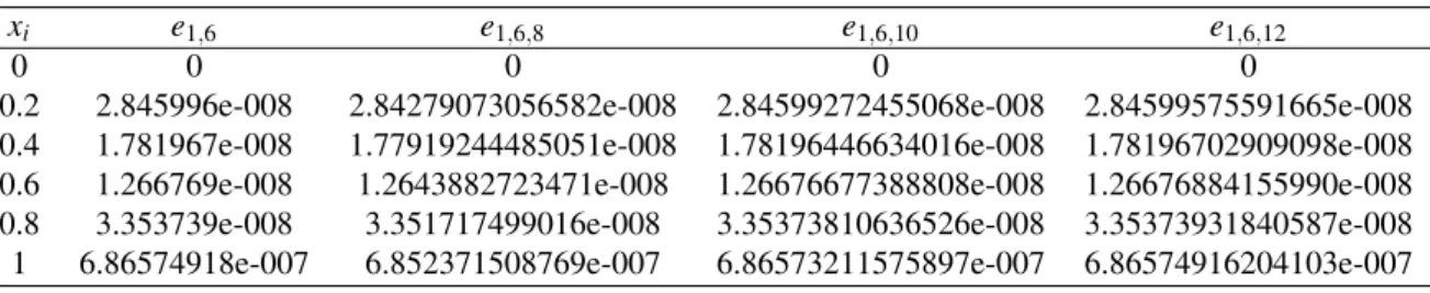
Table 2:Comparison of numerical results of absolute error functione1,6and estimated error functionse1,N,M forM=
8,10,12 of Example2
xi e1,6 e1,6,8 e1,6,10 e1,6,12
0 0 0 0 0
0.2 2.845996e-008 2.84279073056582e-008 2.84599272455068e-008 2.84599575591665e-008
0.4 1.781967e-008 1.77919244485051e-008 1.78196446634016e-008 1.78196702909098e-008
0.6 1.266769e-008 1.2643882723471e-008 1.26676677388808e-008 1.26676884155990e-008
0.8 3.353739e-008 3.351717499016e-008 3.35373810636526e-008 3.35373931840587e-008
1 6.86574918e-007 6.852371508769e-007 6.86573211575897e-007 6.86574916204103e-007
Table 3:Numerical results of absolute error functione2,6of Example2
xi Transform Method [17] Bessel Method [20] Taylor Method [8] Present Method
0 0 0 0 0
0.2 2.3262e-003 2.8460e-008 2.84595e-008 2.8459957e-008
0.4 1.6867e-002 1.7820e-008 1.782165e-008 1.7819678e-008
0.6 5.4499e-002 1.2668e-008 1.26768e-008 1.2667692e-008
0.8 1.3194e-001 3.3538e-008 3.35675e-008 3.3537418e-008
1 2.8038e-001 6.8657e-007 6.865717e-007 6.86574798e-007
Table 4:Comparison of numerical results of absolute error functione2,6and estimated error functionse1,N,M forM=
8,10,12 of Example2
xi e2,6 e2,6,8 e2,6,10 e2,6,12
0 0 0 0 0
0.2 2.8459957e-008 2.84279054342991e-008 2.84599253741479e-008 2.84599556878058e-008
0.4 1.7819678e-008 1.77919322974740e-008 1.78196525123913e-008 1.78196781398054e-008
0.6 1.2667692e-008 1.2643887269948e-008 1.26676722855722e-008 1.26676929615788e-008
0.8 3.3537418e-008 3.351720103513e-008 3.35374071096589e-008 3.35374192277675e-008
Fig. 1:Graphs of absolute error functionse1,Nande2,Nfor valuesN=6,8,10 of Example 2
Example 3.( [2], [6], [8], [20]) Consider the following linear differential system and the condition given with:
y(11)(x) +y(21)(x) +y2(x) =x−e−x
y(11)(x) +4y(21)(x) +y1(x) =1+2e−x
y1(0) =1,y2(0) =0
where 0≤x≤1. Exact solutions of this system arey1(x) =e−x+3e−x/3−3 andy2(x) =−(1/2)e−x+ (3/2)e−x/3−1+x.
Fundamental matrix equation of the problem is
{P0XC∗(1,0)Be+P1XC∗(1,0)DeB}Ae =F
Following the method given in section4we obtain the approximate solutions fori=1,2 andN=5,7,10 as
y1,5(x) =1−2t+0.6665429600045t2−0.1843402224992t3+ (0.409518052792e−1)t4
−(0.569482927692e−2)t5 ,
y2,5(x) =t−0.16660539022198t2+ (0.736556629852e−1)t3−(0.189435481094e−1)t4
+ (0.275727613671e−2)t5 ,
y1,7(x) =1−2t+0.6666662244872t2−0.18518020404123t3+ (0.431857423289e−1)t4
−(0.837418910669e−2)t5+ (0.13056961684e−2)t6−(0.129930152198e−3)t7,
y2,7(x) =t−0.16666644581866t2+ (0.740715862927e−1)t3−(0.200496748775e−1)t4
y1,10(x) =1−2t+0.666666666631961166t2−0.185185184538034076t3
+ (0.43209871008221091e−1)t4−(0.843618659713503e−2)t5+ (0.139451895946467e−2)t6
−(0.1985105812431389e−3)t7+ (0.24580409370444e−4)t8−(0.255863683414e−5)t9
+ (0.17623855808795e−6)t10,
y2,10(x) =t−0.1666666666493146472t2+ (0.74074073750512379e−1)t3
−(0.20061725627686513e−1)t4+ (0.411521264072175e−2)t5−(0.69154388943591e−3)t6
+ (0.989831232911e−4)t7−(0.1227886913003e−4)t8+ (0.1278902468183e−5)t9
−(0.8810722289409e−7)t10 .
Comparison of absolute error values with the ones in [2], [6] and [20] are given in tables 5and 7. We see from these tables that results obtained with present method are better rather than Chebyshev method [2], Stehfest method [6] and they are very close with Bessel Method [20] results. The estimated errors for the error functionse1,6ande2,6are given in
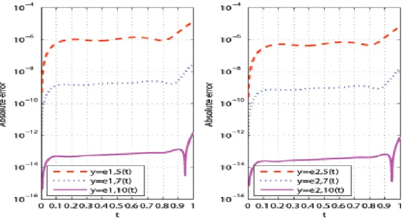
tables 6and 8from which we can see that our estimations are very close to exact errors. In Figure2graphs of the error functionse1,N ande2,N for the valuesN=5,7,10 are given. It is clearly seen from these graphs that errors are decreasing
as the value ofNincreases.
Table 5:Numerical results of absolute error functione1,5of Example3
xi Chebyshev Method [2] Stehfest Method [6] Bessel Method [20] Present Method
0.1 4.510522e-005 6.7614e-005 5.9187e-007 5.9187220e-007
0.2 7.985043e-005 8.4949e-005 1.0110e-006 1.01100956e-006
0.5 9.719089e-005 3.18972e-003 1.0978e-006 1.09778070e-006
0.8 8.006002e-005 5.20283e-003 9.0094e-007 9.0094297e-007
1 1.067677e-004 1.193776e-002 1.3659e-005 1.365938523e-005
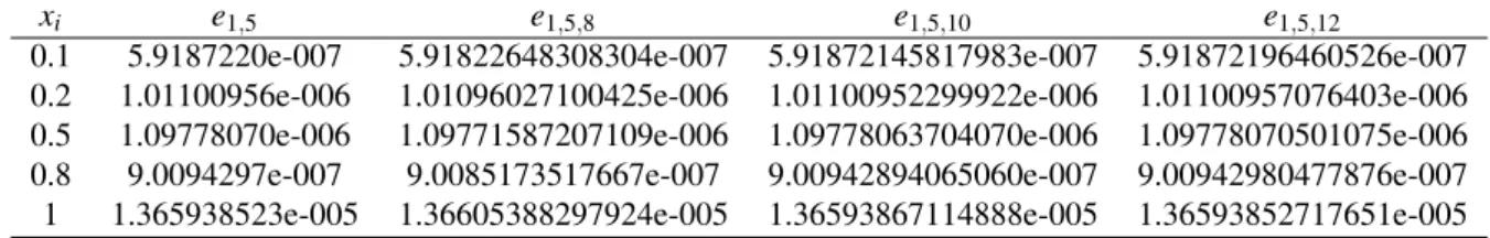
Table 6:Comparison of numerical results of absolute error functione1,5and estimated error functionse1,N,M forM=
8,10,12 of Example3
xi e1,5 e1,5,8 e1,5,10 e1,5,12
0.1 5.9187220e-007 5.91822648308304e-007 5.91872145817983e-007 5.91872196460526e-007
0.2 1.01100956e-006 1.01096027100425e-006 1.01100952299922e-006 1.01100957076403e-006
0.5 1.09778070e-006 1.09771587207109e-006 1.09778063704070e-006 1.09778070501075e-006
0.8 9.0094297e-007 9.0085173517667e-007 9.00942894065060e-007 9.00942980477876e-007
1 1.365938523e-005 1.36605388297924e-005 1.36593867114888e-005 1.36593852717651e-005
Table 7:Numerical results of absolute error functione2,5of Example3
xi Chebyshev Method [2] Stehfest Method [6] Bessel Method [20] Present Method
0.1 2.247723e-005 8.4086e-006 2.9327e-007 2.9327369e-007
0.2 3.984701e-005 1.9575e-005 5.0134e-007 5.0133795e-007
0.5 4.890662e-005 2.242e-004 5.4596e-007 5.4596049e-007
0.8 4.064222e-005 4.647e-004 4.5116e-007 4.5115686e-007
Table 8: Comparison of numerical results of absolute error functione2,5and estimated error functionse1,N,M for M=
8,10,12 of Example3
xi e2,5 e2,5,8 e2,5,10 e2,5,12
0.1 2.9327369e-007 2.93248921695193e-007 2.93273661159323e-007 2.93273687831747e-007
0.2 5.0133795e-007 5.01313313249189e-007 5.01337931456269e-007 5.01337956360630e-007
0.5 5.4596049e-007 5.45928075723713e-007 5.45960451215797e-007 5.45960486276556e-007
0.8 4.5115686e-007 4.5111124446184e-007 4.51156817203302e-007 4.51156861406332e-007
1 6.755515571e-006 6.75609209698840e-006 6.75551629128592e-006 6.75551564509039e-006
Fig. 2:Graphs of absolute error functionse1,Nande2,Nfor valuesN=5,7,10 of Example 3
7 Conclusions
As many kind of problems in applied mathematics are difficult to solve analytically, systems of high-order linear differential-difference equations are so. Because of this issue numerical approaches to solutions of these problem kind are frequently preferred. We choose to use Bernstein polynomials for making an approach to solutions of systems of high-order linear differential-difference equations with variable coefficients under mixed conditions by using nodes which are also called collacation points and converting the problem and the conditions into matrix forms. In some studies because of using collacation points these kind of methods are called as collacation methods as in [8]. Comparing the results in tables 1, 3, 5and 7, we see that present method brings better results rather than Transform method [17],
Chebyshev method [2] and Stehfest method [6] and have very close results with Bessel Method [20] and Taylor
method [8]. From the figures1and2we also see that asNincreases the absolute error values are decreasing. All these shows that our method is efficient and effective. In addition to solving the problem (1) given with the mixed conditions (2), we used residual error function in order to estimate the absolute errors and as seen from the tables 2, 4, 6and 8
References
[1] I.H. Abdel-Halim,Application to differential transformation for solving systems of differential equations, Appl. Math. Modell.,32, 2008, 2552-9.
[2] A. Aky¨uz, M. Sezer,Chebyshev polynomial solutions of systems of high-order linear differential equations with variable coefficients, Appl. Math. Comput.,144, 2003, 237-47.
[3] M.I. Bhatti, P. Bracken,Solutions of differential equations in a Bernstein polynomial basis, J. Comput. Appl. Math.,205, 2007, 272-280.
[4] J. Biazar, E. Babolian, R. IslamSolution of system of ordinary differential equations by Adomian decomposition method, Appl. Math. Comput.,147, 2004, 713-9.
[5] ˙I. C¸ elik,Collacation method and residual correction using Chebyshev series, Applied Mathematics and Computation174, 2006, 910-920.
[6] A. Davies, D. Crann,The solution of systems of differential equations using numerical Laplace transforms,Int. J. Math. Educ. Sci. Technol.,30, 1999, 65-79.
[7] J. Diblik, B.Iricanin, S. Stevic, Z. Smarda,Note on the existence of periodic solutions of a class of systems of differential-difference
equations, Applied Mathematics and Computation, 232 (2014), 922-928.
[8] E. G¨okmen, M. Sezer,Taylor collacation method for systems of high-order linear differential-difference equations with variable
coefficients, Ain Shams Engineering Jornal,4, 2013, 117-125.
[9] H. Jafari, V. Daftardar-Gejji,Revised Adomian decomposition method for solving systems of ordinary and fractional differential
equations, Appl. Math. Comput.,181, 2006, 598-608.
[10] F. Mohamed, I. Naeem, A. Qadir,Conditional linearizability criteria for a system of third-order ordinary differential equations, Nonlinear Anal:Real World Apll.,10, 2009, 3404-12.
[11] FA. Oliveria,Collacation method and residual correction, Numerische Mathematik36, 1980, 27-31.
[12] A. Saadatmandi, M. Denghan, A. Eftekhari,Application of He’s homotopy perturbation method for nonlinear system of second
orer boundary value problems, Nonlinear Anal:Real World Apll.,10, 2009, 1912-22.
[13] M. Sezer, A. Karamete, M. G¨ulsu,Taylor polynomial solutions of systems of linear differential equations with variable coefficients, Int. J. Comput. Math.,82(6), 2005, 755-64.
[14] S. Shahmorad,Numerical solution of general form linear Fredholm-Volterra integro differential equations by the tau method with
an error estimation, Applied Mathematics and Computation167, 2005, 1418-1429.
[15] S. Stevic, J. Diblik, Z. Smarda,On periodic and solutions converging to zero of some systems of differential-difference equations, Applied Mathematics and Computation, 227 (2014), 43-49.
[16] M. Tatari, M. Denghan,Improvement of He’s variational iteration method for solving systems of differential equations, Comput. Math. Appl.,58, 2009, 2160-6.
[17] M. Thangmoon, S. Pusjuso,Numerical solutions of differential transform method and Laplace transform method for a system of
differential equations, Nonlinear Anal: Hybrid Syst.,4, 2010, 425-31.
[18] S¸. Y¨uzbas¸ı,An Efficient algorithm for solving multi-pantograph equation systems, Computers&Mathematics with Applications 64(4), 2012, 589-603.
[19] S¸. Y¨uzbas¸ı, E. G¨ok, M. Sezer,Laguerre matrix Method with the residual error estimation for solutions of a class of delay
differential equations, Math. Meth. Appl. Sci.37, 2014, 453-463.
[20] S¸. Y¨uzbas¸ı, N. S¸ahin, A. Yıldırım,Numerical solutions of systems of high-order linear differential-difference equations with Bessel
polynomial bases, Zeitschrift fr Naturforschung A. J. Phys. Sci.66a, 2011, 519-32.
[21] M. Zurigat, S. Momani, Z. Odibat, A. Alawneh,The homotopy analysis method for handling systems of fractional differential