http://dx.doi.org/10.20852/ntmsci.2016115618
Fibonacci collocation method with a residual error
function to solve linear Volterra integro differential
equations
Ayse Kurt Bahsi and Salih Yalcinbas
Department of Mathematics, Celal Bayar University, Manisa, Turkey
Received: 5 October 2015, Revised: 20 November 2015, Accepted: 7 December 2015 Published online: 1 January 2016.
Abstract: In this paper, a new collocation method based on the Fibonacci polynomials is introduced to solve the high-order linear Volterraintegro-differential equations under the conditions. Numerical examples are included to demonstrate the applicability and validity of the proposed method and comparisons are made with the existing results. In addition, an error estimation based on the residual functions is presented for this method. The approximate solutions are improved by using this error estimation.
Keywords: Volterra integral and integro-differential equations, Fibonacci polynomials, residual error analysis, collocation points, matrix method.
1 Introduction
In recent years, the integral and integro-differential equations have a major role in engineering, mechanics, physics, chemistry, astronomy, biology, economics, potential theory, electrostatics, (Kadalbajoo & Sharma 2002, Elmer & Van Vleck 2002, Maleknejad & Mahmoudi 2004, Cao & Wang 2004, Kadalbajoo & Sharma 2004). A physical event can be modeled by these equations. Since few of these equations cannot be solved explicitly, it is necessary to resort to the numerical techniques. Many authors have worked on numerical methods such as Adomian decomposition method (Wazwaz 2010), the CAS wavelet method (Danfu & Xufeng, 2007), the Galerkin method (Brunner et al, 2009), the Tau method (Pour-Mahmoud, 2005), the finite difference method (Zhao & Corless, 2006), the Haar function method (Maleknejad & Mirzaee, 2006), the sine–cosine wavelet methods (Kajani et al, 2007) for solutions of these equations.
Since the beginning of 1994, for solving the linear and nonlinear Volterra integral and Volterraintegro-differential, Fredholm-Volterraintegro-differential equation matrix methods have also been used by Sezer et al. (Sezer 1994, Yalcinbas & Sezer 2000, Yalcinbas 2002, Sorkun & Yalcinbas 2010, Yuzbasi et al 2011) Also, the Fibonacci matrix method has been used to find the approximate solutions of differential, integral and integro-differential equations, differential- difference equations and Fredholmintegro differential-difference equations (Kurt 2012, Kurt et al 2013a, 2013b).
In this study, we consider the approximate solution of the mth-order Volterraintegro differential equations,
m
∑
k=0
Pk(x)y(k)(x) =g(x) +λ x
∫
a
under the conditions
m−1
∑
k=0
[ajky(k)(a) +bjky(k)(b)] =λj,j=1,2,3, ...,m (2)
wherePk(x),g(x), andK(x,t)are functions defined ona≤x,t≤b;ajk,bjk,λandλjare suitable constants. Our aim is to obtain an approximate solution of (1) expressed in the truncated Fibonacci series form
y(x) =
N
∑
n=1
anFn(x) (3)
an,n=1,2,3, ...,Nare the unknown Fibonacci coefficients. HereNis chosen any positive integer such thatN≥mand
Fn(x),n=1,2,3, ...,Nare the Fibonacci polynomials defined by
Fn(x) =
[(n−1)/2]
∑
j=0 (
n−j−1
j
)
xn−2j−1,
[(n−1)/2] =
{
(n−2)/2,n even
(n−1)/2,n odd.
2 Fundamental matrix relations
We first write the Fibonacci polynomialsFn(x)in the matrix form as follows
FT(x) =CXT(x)⇔F(x) =X(x)CT (4)
whereF(x) = [F1(x)F2(x)...FN(x)],
X(x) = [1x. . .xN−1]
ifNis even,
C= ( 0 0 )
0 0 0 · · · 0
0
( 1 0
)
0 0 · · · 0
( 1 1 ) 0 ( 2 0 )
0 · · · 0
0 ( 2 1 ) 0 ( 3 0 )
· · · 0
..
. ... ... ... ... ... (
(n−2)/2
(n−2)/2 )
0
(
n/2
(n−4)/2 )
0 · · · 0
0
(
n/2
(n−2)/2 )
0
(
(n+2)/2
(n−4)/2 )
· · ·
(
ifNis odd, C= ( 0 0 )
0 0 0 · · · 0
0
( 1 0
)
0 0 · · · 0
( 1 1 ) 0 ( 2 0 )
0 · · · 0
0 ( 2 1 ) 0 ( 3 0 )
· · · 0
..
. ... ... ... ... ...
0
(
(n−1)/2
(n−3)/2 )
0
(
(n+1)/2
(n−5)/2 )
· · · 0
(
(n−1)/2
(n−1)/2 )
0
(
(n+1)/2
(n−3)/2 )
· · · ·
(
n−1 0 ) NxN.
Let us show Eq.(1) in the form
P(x) =g(x) +λI(x) (5)
where
P(x) =
m
∑
k=0
Pk(x)y(k)(x). (6)
3 Matrix relations for the differential part P(X)
We consider the solutiony(x)and its kthderivatey(k)(x)in the matrix form
y(x) =F(x)A,A=[a1a2· · · aN ]T
(7)
y(k)(x) =F(k)(x)A. (8)
Then, from relations (4) and (7), we can obtain the following matrix form
y(x) =X(x)CTA. (9)
Similar to Eq. (8), from relations (4), (7) and (8), we can findy(k)(x)matrix form as
y(k)(x) =X(k)(x)CTA. (10)
To find the matrixX(k)(x)in terms of the matrixX(x),we can use the following relation
X(0)(x) =X(x)
X(2)(x) =X(1)(x)BT = (X(x)BT)BT=X(x)(BT)2
.. .
X(k)(x) =X(k−1)(x)BT=X(x)(BT)k (11)
where
BT =
0 1 0 · · · 0 0 0
0 0 2 · · · 0 0 0
0 0 0 · · · 0 0 0
..
. ... ... ... ... 0 0 0 · · · 0 0 N−1
0 0 0 · · · 0 0 0
.
By using the relations (9)-(11) we have the recurrence relations
y(k)(x) =X(x)(BT)kCTA. (12)
Subsequently, by substituting the matrix form (12) into Eq.(6), we obtain the matrix relations
P(x) =
m
∑
k=0
Pk(x)X(x)(BT)kCTA. (13)
4 Matrix relations for the integral part I(X)
Let us find the matrix relation for the Volterra integral partI(x)in Eq.(6). The kernel functionK(x,t)can be shown by the truncated Fibonacci series,
K(x,t) =
N
∑
m=0 N
∑
n=0
kmnf Fm(x)Fn(t) (14)
and the truncated Taylor series,
K(x,t) =
N
∑
m=0 N
∑
n=0
ktmnxmtn (15)
where
ktmn= 1
m!n!
∂m+nK(0,0)
∂xm∂tn ;m,n=0,1, ...N−1. The expressions (14)-(15) can be put matrix forms as
K(x,t) =F(x)KFFT(t),KF= [
kmnf ] (16)
and
K(x,t) =X(x)KtXT(t),Kt= [
ktmn]. (17)
From (16)-(17) we can obtain
thus
Kt=CTKFC⇒KF= (CT)−1KtC−1. (18)
By substituting the matrix forms (7) and (17) into the integral part I(x)in (5). So we can have the matrix relation as follows
[I(x)] =
x
∫
a
F(x)KFFT(t)F(t)Adt=F(x)KFQ(x)A (19)
so that
[Q(x)] =
x
∫
a
FT(t)F(t)dt=
x
∫
a
CXT(t)X(t)CTdt=CH(x)CT
whereH(x) = [hi j(x)] = x
∫
a
XT(t)X(t)dt,
hi j(x) =
xi+j+1−ai+j+1
i+j+1 i,j=1,2, ...,N. If we subsitute the matrix relation (4) into (19), we have the matrix form
[I(x)] =X(x)MH(x)CTA (20)
where
M=CTKFC.
5 Matrix relations for the conditions
The corresponding matrix form for the conditions (2) can be shown, by means of (12), as
m−1
∑
k=0
[ajkX(a) +bjkX(b)](BT) k
CTA=λj, j=1,2, ...,m. (21)
6 Method of solution
We can construct the fundamental matrix equation corresponding for Eq.(1). For this aim, we substitute the matrix relations (13) and (20) into Eq. (5). So we obtain the matrix equation
m
∑
k=0
Pk(x)X(x)(BT) k
CTA=g(x) +λX(x)MH(x)CTA. (22)
By using in Eq. (22) the collocation pointsxidefined byxi=a+(Nb−−a1)(i−1),i=1,2, . . . ,N.The system of the matrix equations is obtained
m
∑
k=0
Pk(xi)X(xi)CT(BT) k
A=g(xi) +λX(xi)MH(xi)CTA.
or shortly the fundamental matrix equation becomes
{ m
∑
k=0
PkX(BT) k
CT−λX¯M¯H¯C¯
}
A=G (23)
Pk=
Pk(x1) 0 · · · 0 0 Pk(x2)· · · 0
..
. ... . .. 0 0 0 · · · Pk(xN)
, G=
g(x1)
g(x2) .. .
g(xN)
, X=
X(x1)
X(x2) .. .
X(xN) =
1 x1 · · · xN1−1 1 x2 · · · xN2−1
..
. ... . .. ... 1xN · · · xNN−1
, ¯ X=
X(x1) 0 · · · 0 0 X(x2)· · · 0
..
. ... ... ... 0 0 · · · X(xN)
, ¯ M=
M 0 · · · 0 0 M · · · 0
..
. ... ... ... 0 0 · · · M
,C¯=
CT CT .. . CT
, H¯=
Hv(x1) 0 · · · 0 0 Hv(x2)· · · 0
..
. ... ... ... 0 0 · · · Hv(xN)
, A=
a1 a2 .. . aN .
Therefore, the fundamental matrix equation (23) corresponding for Eq. (1) can be written as
WA=G (24)
where
W =
m
∑
k=0
PkX(BT)kCT−λX¯M¯H¯C¯.
Eq. (24) corresponds to a system ofN linear algebraic equations with unknown Fibonacci coefficients a1,a2, ...,aN. Further, we can express the matrix form (21) conditions
UjA= [λj] (25)
where
Uj= m−1
∑
k=0
[ajkX(a) +bjkX(b)](BT) k
CT =[uj1uj2uj3· · ·ujN ]
.
To obtain the solution of Eq. (1) under the conditions (2), by replacing the row matrices (25) by the lastmrows of the matrices (24) (or anymrows of the matrix (24)), we have the new augmented matrix,
[W˜; ˜G] =
w11 w12 · · · w1N ; g(x1)
w21 w22 · · · w2N ; g(x2) ..
. ... ... ... ; ...
w(N−m)1w(N−m)2· · · w(N−m)N ;g(xN−m)
u11 u12 · · · u1N ; λ1
u21 u22 · · · u2N ; λ2
..
. ... ... ... ; ...
um1 um2 · · · umN ; λm
. (26)
If rank ˜W=rank[W˜; ˜G] =N,then we can write
And so, the matrixA(thereby the coefficientsa1,a2, ...,aN) is uniquely determined. Therefore, Eq. (1) with conditions (2) has a unique solution which is given by Fibonacci series solution (3). On the other hand, whenW˜
=0, that is if rank ˜
W=rank[W˜; ˜G]≤N, we can find a particular solution. Otherwise if rank ˜W̸=rank[W˜; ˜G]≤N, then there is no solution.
7 Residual function and error estimation
In this section, we will give an efficient error estimation for the Fibonacci polynomial approximation and also a technique to obtain the corrected solution of the problem (1) and (2) by using the residual correction method (Oliveira 1980, C¸ elik 2006) For our aim, we define the residual function for the present method as
RN(x) = m
∑
k=0
Pk(x)yN(k)(x)−λ x
∫
a
K(x,t)yN(t)dt−g(x) (27)
whereyN(x)is the approximate solution of the problem (1)-(2). Note that,yN(x)satisfies the following problem m
∑
k=0
Pk(x)yN(k)(x)−λ x
∫
a
K(x,t)yN(t)dt=g(x) +RN(x) m−1
∑
k=0
[ajkyN(k)(0) +bjkyN(k)(b)] =λj,j=1,2,3, ...,m.
(28)
In addition, the error functioneN(x)can be defined as
eN(x) =y(x)−yN(x) (29)
wherey(x)is the exact solution of the problem (1) - (2). Substituting (29) into (1) and (2) and using (27) and (28), we have the error differential equation with the homogenous conditions
m
∑
k=0
Pk(x)eN(k)(x)−λ x
∫
a
K(x,t)eN(t)dt=−RN(x) m−1
∑
k=0
[ajkeN(k)(0) +bjkeN(k)(b)] =0,j=1,2,3, ...,m.
(30)
Solving the problem (30) in the same way as in Section 3, we get the approximationeN,M(x)toeN(x),M>Nwhich is the error function based on the residual function.
Subsequently, by means of the Fibonacci polynomialsyN(x)andeN,M(x), we obtain the corrected solution
yN,M(x) =yN(x) +eN,M(x).
Also, we construct the Fibonacci error functioneN(x) =y(x)−yN(x), and the corrected Fibonacci error function
8 Numerical examples
In this section, several examples are given to illustrate the applicability of the Fibonacci matrix method and all of them are performed on the computer. In examples, the terms|eN(x)|and|EN,M(x)|respectively, represent the absolute error function and the absolute error function of corrected Fibonacci polynomial solution.
Example 1.(Kurt 2012) Let us consider the linear Volterraintegro-differential equation given by
(x3−1)y′′(x) +2xy′(x)−y(x) =−2x4+5x3+15x2+3x−7+6 x
∫
0
(x−t)y(t)dt (31)
y(0) =−1,y′(−1) =−5,0≤x,t≤2,
with the exact solution
y(x) =4x2+3x−1. The approximate solutiony(x)by the truncated Fibonacci series
y(x) =
N
∑
n=1
anFn(x)
where
N=4, p0(x) =−1, p1(x) =2x, p2(x) =x3−1, g(x) =−2x4+5x3+15x2+3x−7,λ =6,K(x,t) =x−t.
The collocation points forN=3 are computed as {
x1=0,x2= 2 3, x3=
4 3,x4=2
}
and from Eq.(22), the fundamental matrix equation of the problem is
{
P0XCT+P1X BTCT+P2X(BT) 2
CT−λX¯M¯H¯C¯}A=G.
The augmented matrix for this fundamental matrix equations is
[W;G] =
−1 0 −3 0 ; −7
−73 1027 −20381 −256405; 22381
−193 −2827 1381 2493128 ; 236581
−13 −6 5 5125 ; 67
.
From Eq. (24), the matrix form for the conditions areUjA= [λj]or[Uj;λj];j=0,1 or clearly
[U0;λ0] =[1 0 1 0 ;−1 ]
[U1;λ1] =[0 1−2 5 ;−5 ]
From Eq. (25), we can obtain the new augmented matrix based on the condition as follows
[˜
W; ˜G]
=
−1 0 −3 0 ;−7
−7
3 −
10
27 −
203
81 −
256 405 ;
223 81 1 0 1 0 ;−1 0 1 −2 5 ;−5
.
When we solve this system, we find the Fibonacci coefficients matrix
A=[−5 3 4 0 ]T
Hence, by substituting the Fibonacci coefficients matrix into Eq. (7), we have the approximate solutiony(x) =4x2+3x−1, which is the exact solution.
Example 2.(Yalcinbas & Sezer 2000) Consider the linear Volterraintegro-differential equation
y′(x) =1−
x
∫
0
y(t)dt,0≤x,t≤1 (32)
withy(0) =0 and the exact solutiony(x) =sin(x). From Eq. (23), the fundamental matrix equation is
{
P1X BTCT−λX¯M¯H¯C¯}A=G
whereN=6,p1(x) =1,g(x) =1,λ=−1,K(x,t) =1.Thus, we obtain the solution of the problem forN=6,
y6(x) = (0.762454157653902e−2)x5+ (0.815190187782200)x4
−(0.167011007897479)x3+ (0.519273963677236e−4)x2+x.
In order to estimate the errors forN=6 we consider the following error problem of (30)
e6′(x)−1+ x
∫
0
e6(t)dt=−R6(x)
e6(0) =0.
(33)
Here the residual function is
R(x) =e6′(x)−1+ x
∫
0
e6(t)dt.
By solving the error problem (33) forM=8 introduced in Section 4, the estimated error function approximatione6,8(x) is obtained
e6,8(x) =−(0.179550071001374e−3)x7−(0.346191640591268e−4)x6+ (0.736607283607877e−3)x5
−(0.826804594556656e−3)x4+ (0.346824082083329e−3)x3−(0.521485598362318e−4)x2
+ (0.299239799605999e−14)x+ (0.216840434497101e−18).
Hence, we obtain the corrected exponential solution
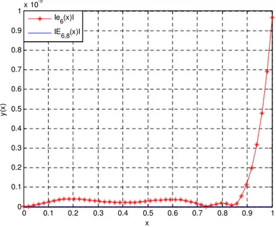
It is seen from Table 1, that the results obtained by the present method is very superior to that obtained by the Taylor method (Yalcinbas & Sezer, 2000). We compare the absolute error|e6(xi)|with the corrected absolute error
E6,8(xi)
in Table 2 which shows the numerical results of the absolute errors and the corrected absolute errors forN=8, M=9. In addition, Figure 1 illustrates a comparison of the absolute error with the corrected absolute error. It indicates the significant decrease in the absolute error owing to the error correction by the residual function
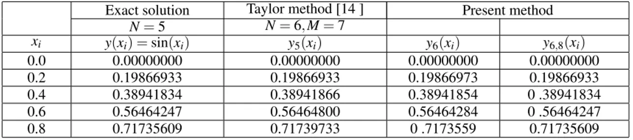
Exact solution Taylor method [14 ] Present method
N=5 N=6,M=7
xi y(xi) =sin(xi) y5(xi) y6(xi) y6,8(xi)
0.0 0.00000000 0.00000000 0.00000000 0.00000000 0.2 0.19866933 0.19866933 0.19866973 0.19866933 0.4 0.38941834 0.38941866 0.38941854 0 .38941834 0.6 0.56464247 0.56464800 0.56464284 0 .56464247 0.8 0.71735609 0.71739733 0 .7173559 0.71735609
Table 1:Comparison of the solutions of Example 5.2.
xi
Absolute error
Corrected absolute error
|e6(xi)|
E6,8(xi)
0.0 0 0
0.2 4.02395202e-7 6.41420e-10 0.4 2.05743865e-7 5.98424e-10 0.6 3.75763114e-7 4.54363e-10 0.8 1.81724658e-7 1.45354e-10 1.0 9.66645529e-6 2.45684e-08
Table 2:Numerical results of the error functions of Example 5.2 forN=8,M=9.
Example 3.(Hosseini & Shahmorad 2002) With exact solutiony(x) =ex2 consider the linear Volterraintegro-differential equation
y′(x) +y(x) =1+2x+
x
∫
0
x(1+2x)et(x−t)y(t)dt,0≤x,t≤1, (34)
y(0) =1.
From Eq. (23), the fundamental matrix equation of the problem is
{
P0XCT+P1X BTCT−λX¯M¯H¯C¯ }
A=G
wherep0(x) =1,p1(x) =1,g(x) =1+2x,λ =1,K(x,t) =x(1+2x)et(x−t).
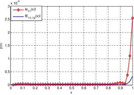
The absolute errors of the solutions obtained by the other methods (Hosseini & Shahmorad 2002, Makroglou 1980)are compared with the absolute error of the solutions obtained by presented method forN=11 in the Table 3. In Table 4 and Figure 3, we compare the corrected absolute error |E11.12(xi)| with the corrected absolute errors |E11.14(xi)| and
0 0.1 0.2 0.3 0.4 0.5 0.6 0.7 0.8 0.9 1 0
0.1 0.2 0.3 0.4 0.5 0.6 0.7 0.8 0.9
1x 10
-5
x
y
(x
)
Ie 6(x)I IE6,8(x)I
Fig. 1:Comparison of the absolute error with the corrected absolute error for Eq.(32).
xi
Tau method (Shahmorad 2005)
Block-by-Block method
(Hosseini & Shahmorad, 2002) Present method
N=10 N=10 N=11,M=12
e10(xi) e10(xi) |e11(xi)| |E11.12(xi)|
0.0 0.000000 0.000000 0.000000 0.000000
0.2 5.721560e-12 3.630000e-8 2.766215e-8 7.344930e-9 0.4 2.384510e-8 1.600000e-7 2.505511e-8 6.86885e-9 0.6 1.049210e-4 4.450000e-7 2.342665e-8 6.05788e-9 0.8 1.049210e-4 1.110000e-6 2.324619e-8 3.58465e-9 1.0 1.615160e-3 2.750000e-6 2.553052e-6 3.33466e-7
Table 3:Comparison of the absolute errors of Eq. (34).
xi Corrected absolute error
|E11.12(xi)| |E11.14(xi)| |E11.17(xi)|
0 0 0 0
0.2 7.34493e-9 9.1127e-10 2.8085e-10 0.4 6.86885e-9 9.9376e-10 7.151e-11 0.6 6.05788e-9 5.3919e-10 3.8486e-10 0.8 3.58465e-9 8.8155e-10 2.71137e-9 1.0 3.33466e-7 1.6776e-7 3.98625e-9
Table 4:Numerical results of the error functions of Example 5.3 forN=11,M=12,14,17.
c
0 0.1 0.2 0.3 0.4 0.5 0.6 0.7 0.8 0.9 1 0
0.5 1 1.5 2 2.5
3x 10
-6
x
y
(x
)
Ie11(x)I
IE11,12(x)I
Fig. 2:Comparison of the absolute error with the corrected absolute error for Eq.(34).
0 0.1 0.2 0.3 0.4 0.5 0.6 0.7 0.8 0.9 1
0 0.5 1 1.5 2 2.5 3 3.5x 10
-7
x
y
(x
)
IE11,12(x)I
IE11,14(x)I
IE11,17(x)I
Fig. 3:Comparison of the corrected absolute errors for Eq.(34).
9 Conclusion
In this article, we have presented Fibonacci collocation method with a residual error function to solve high order linear Volterra integro-differential equations. From the comparisons of the results obtained by this method is more effective than some other methods. It is observed from discussed examples which have the exact solution, the error estimation algorithm is very effective when the compared absolute errors of these examples. And also, if the exact solution of the problem is
c
unknown, the absolute errors can be computed with this error estimation algorithm. One of the considerable advantages of this method is that the approximate solutions are found very easily by using the computer programs. As seen from this study, the Fibonacci polynomial approach is a good approximation for solving these equations.
References
[1] Brunner H., Davies P.J & Duncan D.B. 2009. Discontinuous Galerkin approximations for Volterra integral equations of the first kind.IMA J. Numer. Anal.29: 856–881.
[2] Cao J. & Wang J. 2004. Delay-dependent robust stability of uncertain nonlinear systems with time delay.Appl. Math. Comput. 154: 289–297.
[3] C¸ elik ˙I. 2006. Collocation method and residual correction using Chebyshev series.Applied Mathematics and Computation. 174 (2): 910-920.
[4] Danfu H. & Xufeng S. 2007. Numerical solution of integro-differential equations by using CAS wavelet operational matrix of integration.Appl. Math. Comput. 194: 460–466.
[5] Elmer C.E. & Van Vleck E.S. 2002. A variant of Newton’s method for solution of traveling wave solutions of bistable differential-difference equation.J. Dyn. Differ. Equ.14: 493–517.
[6] Erdem K., Yalcinbas S., Sezer M. 2013. A Bernoulli approach with residual correction for solving mixed linear Fredholmintegro-differential-difference equations,Journal of Difference Equations and Applications, 19(10): 1619-1631.
[7] Hosseini S.M. &Shahmorad S. 2002. A matrix formulation of the Tau method and Volterra linear integro-differential equations. Korean J. Comput. Appl. Math.9 (2): 497–507.
[8] Kadalbajoo, M.K. & Sharma K.K. 2002. Numerical analysis of boundary-value problems for singularly-perturbed differential-difference equations with small shifts of mixed type.J. Optim. Theory Appl.115: 145–163.
[9] Kadalbajoo M.K. & Sharma K.K. 2004. Numerical analysis of singularly-perturbed delay differential equations with layer behavior.Appl. Math. Comput.157:11–28.
[10] Kajani M.T., Ghasemi M. &Babolian E. 2007. Comparison between the homotopy perturbation method and the sine–cosine wavelet method for solving linear integro-differential equations.Comput. Math. Appl.54: 1162–1168.
[11] Kurt A. 2012. Fibonacci polynomial solutions of linear differential, integral and integro-differential equations, M.Sc. Thesis, Graduate School of Natural and Applied Sciences, Mugla University.
[12] Kurt A., Yalcinbas S. &Sezer M. 2013. Fibonacci Collocation Method For Solving Linear Differential-Difference Equations. Mathematical and Computational Applications.18.3: 448-458.
[13] Kurt A., Yalc¸ınbas¸ S., Sezer M. 2013. Fibonacci Collocation Method for Solving High- Order Linear FredholmIntegro-Differential-Difference Equations.International Journal of Mathematics and Mathematical Sciences2013: 1-9.
[14] Makroglou A. 1980. Convergence of a block-by-block method for nonlinear Volterraintegro differential equations, Math. Comput.35: 783–796.
[15] Maleknejad K. &ahmoudi Y. 2004. Numerical solution of linear Fredholm integral equation by using hybrid Taylor and block-pulse functions.Appl. Math. Comput. 149: 799–806.
[16] Maleknejad K. &Mirzaee F. 2006. Numerical solution of integro-differential equations by using rationalized Haar functions method.Kybernetes Int. J. Syst. Math. 35: 1735–1744.
[17] Oliveira FA. 1980. Collocation and residual correction. NumerischeMathematik, 36 (1): 27-31.
[18] Pour-Mahmoud J., Rahimi-Ardabili M.Y & Shahmorad S. 2005. Numerical solution of the system of Fredholmintegro-differential equations by the Tau method.Appl. Math. Comput.168: 465–478.
[19] Sezer M. 1994. Taylor polynomial solution of Volterra integral equations.Int. J. Math. Educ. Sci. Technol.25: 625–633.
[20] Shahmorad S. 2005. Numerical solution of general form linear Fredholm-Volterraintegro-differential equations by the Tau method with an error estimation.Appl. Math. Comput.167 (2): 1418-1429.
[22] Wazwaz A.M. 2010. The combined Laplace transform-Adomian decomposition method for handling nonlinear Volterraintegro-differential equations.Appl. Math. Comput. 216: 1304–1309.
[23] Yalcinbas S. & Sezer M. 2000. The approximate solution of high-order linear Volterra–Fredholmintegro-differential equations in terms of Taylor polynomials.Appl. Math. Comput. 112(2): 291–308.
[24] Yalcinbas S. 2002. Taylor polynomial solutions of nonlinear Volterra-Fredholm integral equations.Appl. Math. Comput. 127: 195-206.
[25] Yalcinbas S. & Erdem K. 2010. Approximate solutions of nonlinear Volterra integral equation systems.International Journal of Modern Physics B, 24(32): 6235-6258.
[26] Yalcinbas S., Sahin N. & Sezer M. 2011. Bessel polynomial solutions of high-order linear Volterraintegro-differential equations. Comput. Math. Appl. 62(4): 1940-1956.