Theoretical and numerical characterization of continuously graded thin layer by the reflection acoustic microscope

(1)

Theoretical and numerical characterization of

continuously graded thin layer by the reflection

acoustic microscope

Ahmed Markou, Hassan Nounah and Lahcen Mountassir

Laboratory of Metrology and Information Processing

Department of Physics

Faculty of Sciences, Ibno Zohr University, Agadir, Morocco

Abstract—This article presents a theoretical and numerical

study by the reflection acoustic microscope of the surface acoustic waves propagation at the interface formed by a thin layer and the coupling liquid (water). The thin layer presents a gradient in its acoustical parameters along its depth. A stable transfer matrix method is used to compute the reflectance function of the surface acoustic modes radiated in the coupling liquid. This function is required to calculate the theoretical acoustic material signature which allows to determine the phase velocity of these modes. In order to characterize the influence of the gradient on the acoustic material signature, a few gradient functions are studied. The numerical results obtained show that the acoustic material signature can be used to characterize these profiles.

Keywords—Reflection acoustic microscope; Surface acoustic

wave; Thin graded layer; Transfer matrix method; Reflectance function; Acoustic material signature

I. INTRODUCTION

The acoustic microscope is an ultrasonic wave sensor, at the presence of an electrical excitation in its input allows to generate an acoustic wave capable to penetrate into the structures with a high resolution. This device is widely used in the various fields of nondestructive testing, such as mi-croelectronics [1] and metallurgy [2] and biology [3], etc. The development of the first acoustic scanning microscope is motivated by the idea of using the acoustic field to study the elastic properties of materials with a resolution equivalent or better than that obtained by the optical microscope [4]. The acoustic material signature or V(z) curve has been used by Atlar et al. [5] to analyze the images obtained by the reflection acoustic microscope. They have obtained the V(z) curve by recording the voltage in the output of the transducer at each defocus z (distance between the acoustic lens and the sample). Weglein et al. [6] found that the periodic oscillations in the V(z) curve are linked to the surface acoustic wave propagation. Parmon and Bertoni proposed a simple formula, by using a ray model, to calculate the velocity of the surface acoustic wave from measuring the period of the oscillations in the V(z) curve [7]. The invention of the line focus acoustic microscope allows the quantitative measurement of the elastic properties and thicknesses of isotropic and anisotropic layered materials [8][9]. Today many techniques concerning the quantitative measurement by the acoustic microscope are developed to characterize the elastic properties of different solids. These techniques involve many type of acoustic microscope, cit-ing for example: the conventional acoustic microscope and

time-resolved acoustic microscope [10] and tow-lens acoustic microscope. For the conventional acoustic microscope, the acoustic beam is focused onto a sample by means of an acoustic lens. The transducer is located on the upper part of this lens and its other face is ground into a cavity with a quarter-wavelength matching layer. According to the shape of this cavity, we can distinguish tow conventional acoustic microscope types: line focus acoustic microscope (LFAM) which has a cylindrical cavity form. This lens focuses the acoustic wave along a line and the surface acoustic wave are excited in the direction perpendicular to the focal line. For the acoustic microscope with a spherical cavity shape, the wave is focused onto a spot with the dimensions comparable to the acoustic wavelength in the coupling liquid, which is placed between the lens and the specimen. In this study we will focus on the numerical investigation of the acoustic material signature by the reflection acoustic microscope with spherical cavity to evaluate the influence of the gradient function shape on V(z) curve and on its phase for the continuously thin graded layer on a solid substrate. The numerical example considered in this article is a thin graded Aluminum layer deposited in a solid Silicon substrate, where the Aluminum layer presents a continuous gradient in its elastic parameters and density, from its surface to a given depth (layer thickness). For modeling the inhomogeneous area, a simple gradient functions are used to describe the variation of the elastic properties according to the spatial coordinate. There are several methods for determining the reflectance functionR(f, θ)relative to the inhomogeneous media, such as transfer matrix method and stiffness matrix method [11] and Peano series expansion [12], etc. The model adopted in this study to evaluate the surface acoustic wave propagation is based on the transfer matrix formalism which is detailed in the previous study [13]. The present study offers the possibility to characterize the gradient profiles in the elastic properties of a thin layer by the V(z) curve technique and by the dispersion curve of the surface acoustic wave. The first stage is to establish the reflectance function [13] and the second stage is to determine the expression of the V(z) curve (section II) and deducing the dispersion curve.

II. BACKGROUND THEORY

There are several methods for analyzing the V(z) curve in the output of a focus transducer for the solid structures and this section will expose Auld and Weise et al. and Zinin et al. approaches for determining V(z) curve expression

(2)

[14][15][16][17].

The figure 1 shows the defocused acoustic lens schema for a reflection acoustic microscope. The trajectoryCOis related to the specular wave and BF HD is the trajectory of the leaky surface acoustic wave (in the ray model). The leaky Rayleigh wave is excited by the ray BF, finally the trajectory AO′

E

is relative to the edge wave . The acoustic lens is moved mechanically away the sample in the positive values of z. The following assumption is considered: the coupling liquid is parfait and then does not support transverse modes and that the sample is a solid plan reflector.

Fig. 1. Defocused acoustic lens in the reflection acoustic microscope

The output signalV of the reflection acoustic microscope at any positionz can be expressed as [18]:

V =

Z −∞

∞

Z −∞

∞

Uin(−k1,−k2)Usc(k1, k2)k3dk1dk2 (1)

WhereUinandUsc are, respectively, the Fourier spectrum of

the incident and scattered acoustic fields.k1andk2andk3are

the components of the wave-vectork, wherek=ω/vliq.ω is

the angular frequency andvliqis the acoustic wave velocity in

the coupling liquid. In the Debye approximation, the spectrum of the incident field at the focal plane can be written as:

Uin=

P(k1, k2)

k3

(2)

With P(k1, k2)represents the pupil function, it is defined as

the distribution of the field emitted before crossing the lens. The Fourier spectrum of the acoustic field reflected from a multi-layered system located between tow semi-infinite media is as following [19]:

Usc=R(k1, k3)Ui(k1, k2) (3)

At the object plane marked byzcoordinate, the expression of the spectrum of the incident field is determined by intro-ducing the propagation factorexp(jk3z). Taking into account

the equation (1) and (2) and (3), the expression of the output signal V(z) is then:

V(z) =

Z −∞

∞

Z −∞

∞

P(−k1,−k2)P(k1, k2)

×R(k1, k3) exp(2jk3z)dk1dk2/k3

(4)

The expression of the V(z) in the equation (4) is relative to an anisotropic sample in the non-par-axial approximation.

For an acoustic microscope with spherical lens and taking into account the spherical coordinates and the Debye approach which consider that pk2

1+k22 ≤ sinθm. Where θm is the

semi-aperture of the pupil. For symmetrical pupil function, the V(z) curve can be expressed as (the constant resulting from the second integral on the azimuthal angleφis omitted) :

V(z) =

Z θm

0

P2(θ)R(θ, ω) exp(2jkzcos(θ)) cosθsinθdθ

(5)

R(θ, ω) is the reflectance function of the acoustic wave propagating at the interface constituted by the coupling liquid and the graded layer. This reflectance is of great importance because it contains all informations about the modes which are reflected in the coupling liquid.

According to the ray model, which consider only the contribution of the normal rays to the lens surface of the acoustic microscope, the velocity of the surface acoustic wave

vSAW and the periodicity in the acoustic material signature

V(z), for each given frequencyf, are related by the following formula:

vSAW =

vliq

q

1−(1− vliq

2f∆z)2

(6)

Where∆zrepresents the period of the oscillations in the V(z) curve. This period can be calculated by using the fast Fourier transform of the windowing V(z) curve.

III. NUMERICAL RESULTS AND DISCUSSION

A. Gradient functions

The numerical values of the ultrasonic velocities and densities of the layer and substrate [20] used in numerical simulations are regrouped in the following table:

TABLE I. INPUT DATA USED IN SIMULATION

VL(m/s) VT(m/s) ρ(kgm−1) d(µm)

Silicon 8485 5850 2300

-Aluminum 6374 3111 2700 10

water 1500 - 1000

-The gradient functions used in simulations are:

fl(x3) =f0+ (fd−f0)x3

fg(x3) =f0exp(−αx23)

ftanh(x3) =f0+ (fd−f0)a1

a2

(7)

Where fl and fg and fT anh are, respectively, the linear

and Gaussian and tanh profiles, they describe the physical properties along the depth x3.d denotes the thickness of the

graded layer.f0andfdare the acoustical parameters at the top

surface of the layer (x3= 0) and at the substrate (x3=d).α

anda1 anda2 are defined as the following:

α=1

d2log(

f0

fd

)

a1=tanh(b(x3−

d

2))−tanh(b

d

2)

a2=tanh(b(

d

2)−tanh(−b(

d

2))

(8)

(3)

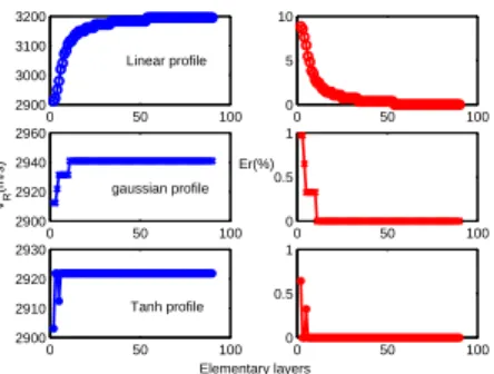
With b is a given constant, it allows to provide different Tanh profile shapes. To approach the physical reality of a continuously graded layer, the thin layer is divided into a finite number n of homogeneous elementary layers. For each subdivision n and at a fixed frequency, the phase velocity of the leaky Rayleigh wave which propagates in the layer is determined. When this velocity becomes stable and remains unchanged with n, its convergence is reached. The asymptotic value reached by the phase velocity allows to estimate the relative error related to the convergence.

The figure 2 shows the longitudinal velocity profiles given by the functions in the relationship (7), where these velocity profiles vary between the tow values of the longitudinal velocities in the Aluminum (top surface of the layer) and in the Silicon (in the substrate). The transversal velocity and density are also varied in the direction perpendicular to the surface of layer and follow the same profiles as those presented in the figure 2.

0 2 4 6 8 10 6000

6500 7000 7500 8000 8500

x₃(µm)

Longitudinal velocity(m/s)

Linear profile Gaussian profile Tanh profile

Fig. 2. Gradient functions simulating the gradient of the layer,d= 10µm

Each point in the figure 2 corresponds an homogeneous elementary layer with thickness equal to 0.5µm. As mention this figure, the graded layer is discretized then into twenty elementary layers.

0 50 100 2900

3000 3100 3200

0 50 100 0

5 10

0 50 100 2900

2920 2940 2960

Elementary layers

VR

(m/s)

0 50 100 0

0.5 1

0 50 100 2900

2910 2920 2930

0 50 100 0

0.5 1 Linear profile

gaussian profile

Tanh profile Er(%)

Fig. 3. Convergence of the velocityVR(blue) and its error (red) versus the

number of elementary layersnat f=1GHz

The figure 3 shows the convergence of the phase velocity of the leaky Rayleigh mode (blue curve) and its relative error (red curve) versus the number of elementary layers at the frequency of 1GHz. From analyzing this figure, it is clear that the number of elementary layers is justified by the convergence of the Rayleigh velocity. Indeed, for a linear profile and at the frequency of 1GHz for to have an error less than 1% on the phase velocity of the leaky Rayleigh mode, the graded

layer should be slicing into about twenty elements (figure 3). For the other profiles like Gaussian and Tanh, the stabilization of the phase velocity of the leaky Rayleigh mode is reached when the layer is subdivided into about only ten elements. At low frequency (10MHz), the phase velocity of the leaky Rayleigh mode stabilizes at few elementary layers (n=2 for linear profile and n=4 for the Tanh profile). For the Gaussian profile, this velocity remains constant versus the number of elementary layers (figure 4).

0 5 10 15 5080

5100 5120 5140

0 5 10 15 0

0.5 1

0 5 10 15 5065

5066 5067 5068

0 5 10 15 −1

0 1

0 5 10 15 5080

5100 5120 5140

0 5 10 15 0

0.5 1

Elementary layers Er(%)

VR

(m/s)

Linear profile

Gaussian profile

Tanh profile

Fig. 4. Convergence of the velocityVR(blue) and its error (red) versus the

number of elementary layersnat f=10MHz

The following points explain the results in the figures 3 and 4:

• At high frequency (f=1GHz) and for great values of slicingninto elementary layers, the thickness∆x3=

d/n of each element becomes small with regards to the wavelength and gives almost continuous variation of the acoustic parameters∆fi and thenVRbecomes

steady. For∆x3large (nis small), the properties (∆fi

important) of the layer vary discontinuously, thing that lead to a sharp variation in the velocityVR

• At low frequency (f=10MHz), the wavelength of the leaky Rayleigh wave is very important in comparison with the global thickness of graded layer and then the depth of penetration of the acoustic wave is large and then the disturbance due to the gradient is negligible. This fact leads to the fast convergence of the velocity of the leaky Rayleigh modeVR.

B. Acoustic material signature and dispersion curve

The images in the figures 5 and 6 (left figures) represent the phase of the reflectance function R(f, θ) plotted in the plan (f, θ). They show the dispersion of different surface acoustic modes radiated in the coupling liquid. The first mode in these images is called leaky Rayleigh mode, and the other modes are called Sezawa modes. As mention these figures, their phases vary between the tow values−πand+π. In the dispersion curve relative to the linear profile (figure 5 left), the first sezawa mode presents a cut off frequency at the frequency of 280MHz where the phase velocity is about 5850 m/s (θ=14.84 degree), which is also the value of the transversal velocity in the substrate. The mode which corresponds to the phase velocity above the transversal velocity in the substrate is called pseudo-Sezawa mode. For the other profiles, the second mode is continuous and does not show the discontinuity observed in the dispersion curve relative to the linear profile. These images show also that the

(4)

−3 −2 −1 0 1 2 3

Frequency(MHz)

Incident angle(

°

)

0 200 400 600 800 1000

0

10

20

30

40

50

Phase R

−3 −2 −1 0 1 2 3

Frequency(MHz)

Incident angle(

°

)

0 200 400 600 800 1000

0

10

20

30

40

50

Phase R

Fig. 5. Phase of the reflectance functionR(f, θ)relative to the linear profile (left) and for the Gaussian profile (Right)

−3 −2 −1 0 1 2 3

Incident angle(

°

)

Frequency(MHz)

0 200 400 600 800 1000

0

10

20

30

40

50

Phase R

0 200 400 600 800 1000

2500 3000 3500 4000 4500 5000 5500

Frequency(MHz)

Phase velocity(m/s)

Linear profile gaussian profile Tanh profile

Fig. 6. Phase of the reflectance functionR(f, θ)relative to the Tanh profile (left) and the dispersion curve of Rayleigh mode (right) for the three profiles

0 500 1000 1500 2000

0 0.2 0.4 0.6 0.8 1

Defocus(µm)

Normalized amplitude

linear profile Gaussian profile Tanh profile

f= 47.5MHz

0 100 200 300 400 500 600

−4 −3 −2 −1 0 1 2 3 4

Defocus(µm)

Phase

Fig. 7. Variations of V(z) curve (left) and its phase (right) relative to the three profiles simulating the graded layer at the frequency of 47.5MHz

0 500 1000 1500 2000

0 0.1 0.2 0.3 0.4 0.5

Defocus(µm)

f=200MHz

400 420 440 460 480 500

−3 −2 −1 0 1 2 3 4

Defocus(µm)

Phase

f=200MHz

Fig. 8. Variations of V(z) curve (left) and its phase (right) relative to the three profiles simulating the graded layer at the frequency of 200MHz

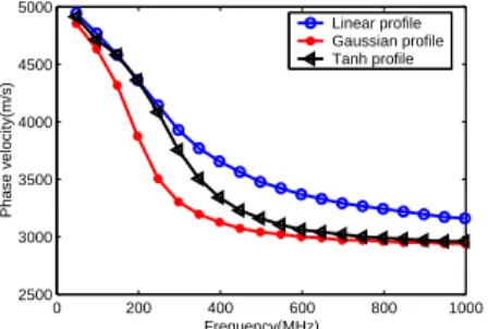
number of the surface acoustic modes which appear in the dispersion curve differs from a profile to an other. The figure 6 (right) shows the dispersion curve of the leaky Rayleigh modes for the three gradient profiles, where the phase velocity of the modes vary between 5163 m/s at low frequency (2.5 MHz) and 3160 m/s for linear profile and about 2900 m/s for Tanh and Gaussian profiles at high frequency (1GHz). Below 100MHz the influence of gradient function is very less. This influence appears at high frequencies. From the frequency of 800MHz, the dispersion curve relative to the Gaussian and Tanh profiles are confused, this because of the gradient

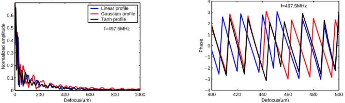
functions which are identical near to surface layer (figure 2). The figures 7 and 8 and 9 show the theoretical V(z) curve (left) and its phase (right) for the three gradient functions used in the simulations. They show the influence of the shape of the gradient functions on the V(z) curve and on its phase. At low frequencies (below 100MHz), this influence is almost null. Above the frequency of 100MHz, the effect of the gradient appears and a lag between the peaks in the phase of V(z) curve appears for the three profiles (figure 8 et 9 left). These peaks are relative to the leaky surface acoustic modes. It is also possible to study these profiles by the V(f) curve which

(5)

0 200 400 600 800 1000 0

0.1 0.2 0.3 0.4 0.5 0.6

Defocus(µm)

f=497.5MHz

400 420 440 460 480 500

−4 −3 −2 −1 0 1 2 3 4

Defocus(µm)

Phase

f=497.5MHz

Fig. 9. Variations of V(z) curve (left) and its phase (right) relative to the three profiles simulating the graded layer at the frequency of 497.5MHz

0 200 400 600 800 1000

0 0.2 0.4 0.6 0.8 1

Frequency(MHz)

z= 8.57µm

0 200 400 600 800 1000

−4 −3 −2 −1 0 1 2 3 4

Frequency(MHz)

Phase

z= 8.57µm

Fig. 10. Variations of V(f) curve (left) and its phase (right) relative to the three profiles simulating the graded layer at the defocus of 8.57µm

0 200 400 600 800 1000

0 0.2 0.4 0.6 0.8 1

Frequency(MHz)

z= 34.29µm

300 350 400 450 500

−4 −3 −2 −1 0 1 2 3 4

Frequency(MHz)

Phase

z= 34.29µm

0 100 200 300 400 500 600 700 800

0 0.2 0.4 0.6 0.8 1

Frequency(MHz)

z=568.57µm

700 720 740 760 780 800

−4 −3 −2 −1 0 1 2 3

Frequency(MHz)

Phase

z= 568.57µm

0 200 400 600 800 1000

0 50 100 150 200 250 300 350

Frequency(MHz)

∆

z(

µ

m)

0 200 400 600 800 1000

0.4 0.6 0.8 1 1.2 1.4

1.6x 10

4

Frequency(MHz)

∆

z

×

f(m.Hz)

Fig. 13. Variations of the period∆z(left) andf∆z(right), relative to the Rayleigh mode, with the frequency for the three gradient profiles

(6)

is calculated by setting the defocus z and by varying the frequencyf in the integral of the equation 5. The V(f) curve (left) and its phase (right) are presented in the figures 10, 11 and 12. These figures show the variations of the V(f) curve and its phase versus the frequency at the fixed defocus. The difference between these curves, relative to the three profiles, is more pronounced above the frequency of 100MHz. For interpreting all these remarks, we use the dispersion curve in the figure 6 (right). Indeed, at the frequency of 100MHz, the phase velocity of the leaky Rayleigh mode, for the linear and Gaussian and Tanh profiles are, respectively, 4796 m/s and 4660 m/s and 4741 m/s which correspond to the wavelength ofλ123=(53.3µm, 51.78µm, 52.68µm). These wavelength are

five times higher than the layer thickness (d=10µm). Then the acoustic wave ”sees” the graded layer as homogeneous and then the effect of the gradient functions on the acoustic wave is negligible. When the wavelength, relative to the three profiles, approaches or exceeds the layer thickness (at f=300MHz, λ123 =(13.1µm, 11µm, 12.5µm )), the acoustic

wave is more influenced by the graded area in the thickness of the layer and its propagation becomes dependent to the frequency.

The reflection acoustic microscope offers the possibility to characterize the gradient profiles through the analyze of the dispersion curve which can be determined from the V(z) curve by calculating different periods in this curve. The figure 13 shows the period∆z(left) and the quantityf∆z(right) versus the frequency. For the leaky Rayleigh mode,∆z is calculated from the tow first successive minima at each frequency in the V(z) curve. The quantity f∆z has the same shapes as the phase velocity VR, but its values can be determined by the

relationship (6) (figure 14).

0 200 400 600 800 1000

2500 3000 3500 4000 4500 5000

Frequency(MHz)

Phase velocity(m/s)

Fig. 14. Dispersion curve ofVRcalculated from the equation 6

IV. CONCLUSION

This work presents a theoretical and numerical model of the characterization, by reflection acoustic microscope, of unidirectional continuous gradient profile in acoustical prop-erties of thin layer. For to be close to the physical reality of a continuously inhomogeneous media, the graded layer is divided into a finite number of homogeneous elementary layers of equal thicknesses. This number is selected in such a way to have a compromise between the accuracy of results and the computing time. A number of twenty elementary layers ensures an error of 1% in the leaky Rayleigh velocity. This result is used to calculate the V(z) and V(f) curves according to the wave theory exposed in the section II. The interest of these tow curves is that they allow the determination of the

dispersion curve of the surface acoustic wave by evaluating the periodicity of the V(z) curve at each frequency. The analyze of the dispersion curve of leaky Rayleigh mode and the V(z) curve, for the three gradient profiles, studying in this work, show a clear dependence of the acoustic wave propagation to the frequency when the thickness of the graded layer is the same order of magnitude as the acoustic wavelength.

REFERENCES

[1] D. A. Hutt, D. P. Webb, K. C. Hung, C. W. Tang, P. P. Conway, D. C. Whalley and Y. C. Chan,Scanning Acoustic Microscopy Investigation of Engineered Flip-chip Delamination, 26th IEEE/CPMT International Electronics Manufacturing Technology Symposium, California, pp.191-199, 2000.

[2] C. Pecorari, P. B. Nagy and L. Adler,Acoustic microscopy to study grain structure, Review of Progress in Quantitative Nondestructive Evaluation. Vol. 09, Plenum Press : New York, 1990.

[3] C. F. Quate, A. Atalar and H. K. Wickramasinghe,Acoustic Microscopy With Mechanical Scanning-A Review, Proceedings of IEEE. Vol. 67 No. 8, 1979.

[4] R. A. Lemons and C. F. Quate,Acoustic Microscopy, Physical Acoustics Vol. XIV, Mason, London Academic, 1979.

[5] A. Atalar, C. F. Quate and H. K. Wickramasinghe,Phase imaging in reflection with the acoustic microscope, Appl. Phys. Lett. 31(12) p. 791-793, 1977.

[6] R. D. Weglein and R. G. Wilson,Characteristic material signatures by acoustic microscopy, Electron.Lett .14(12) pp.352-354, 1978. . [7] W. Parmon and H. L. Bertoni,Ray interpretation of the material signature

in the acoustic microscope, Electron.Lett.15(12) pp. 684-686, 1979. [8] J. Kushibiki, A. Ohkubo and N. Chubachi Linearly focused acoustic

beams for acoustic microscope, Electron.Lett.17(15) pp. 520-522, 1981. [9] J. Kushibiki, A. Ohkubo and N. ChubachiAnisotropy detection in sap-phire by acoustic microscope using line-focus beam, Electron.Lett.17(15) pp. 534-536, 1981.

[10] E. C. Weiss, P. Anastasiadis, G. Pilarczyk, R. M. Lemor and P. V. Zinin, Mechanical Properties of Single Cells by High-Frequency Time-Resolved Acoustic Microscopy, IEEE Transactions On Ultrasonics, Ferroelectrics, and Frequency Control, Vol.54, No.11, pp.2257-2271, 2007.

[11] X. Deng, T. Monnier, P. Guy and J. Courbon, Acoustic microscopy of functionally graded thermal sprayed coatings using stiffness ma-trix method and Stroh formalism, J.Appl.Phys.113(22), pp.224508:1-10, 2013.

[12] C. Baron, Series expansion of the matricant for studying the elastic waves propagation in the mediums with continuously variable properties, PhD dissertation, Bordeaux, France, 2005.

[13] A. Markou and H. Nounah,Numerical Evaluation of the Effect of Gra-dient On reflection Coefficient of Continuously Graded Layer, IJACSA, Vol.6(5), pp.97-102, 2015.

[14] A. Atalar, An angular spectrum approach to contrast in reflection acoustic microscopy, J. Appl. Phys. 49(10), pp.5130-5139, 1978. [15] B. A. Auld,general electromechanical reciprocity relations applied to

the calculation of elastic wave scattering coefficients, Wave Motion 1:3-10, 1979.

[16] W. Weise, P. Zinin and S. Boseck,Angular spectrum approach for imag-ing spherical-particles in reflection and transmission scannimag-ing acoustic microscope, Acoustical imaging, pp.707-712 vol.22, Plenum: New York, 1996.

[17] P. Zinin, W. Weise, O. Lobkis and S. Boseck , The theory of three-dimensional imaging of strong scatterers in scanning acoustic micro-scope, Wave Motion 25(3):213-236, 1997.

[18] A. Atalar,A backscattering formula for acoustic transducers, J. Appl. Phys.51(6)pp. 3093-3098, 1980.

[19] W. Weise, P. Zinin and S. BoseckModeling of inclined and curved surfaces in the reflection scanning acoustic microscope, J. microsc.176(3) pp. 245-253, 1994.

[20] H. Nounah,Modeling and characterization of materials with gradient in the mechanical properties by the micro acoustic methods, PhD dissertation, Montpellier II, France, 1995.