www.geosci-model-dev.net/6/2023/2013/ doi:10.5194/gmd-6-2023-2013
© Author(s) 2013. CC Attribution 3.0 License.
Geoscientiic
Model Development
A hybrid Eulerian–Lagrangian numerical scheme for solving
prognostic equations in fluid dynamics
E. Kaas1, B. Sørensen1, P. H. Lauritzen2, and A. B. Hansen3,4 1Niels Bohr Institute, University of Copenhagen, Copenhagen, Denmark 2Climate and Global Dynamics Division, Boulder, Colorado, USA
3Aarhus University, Department of Environmental Science, Roskilde, Denmark 4National Institute of Water and Atmospheric Research, Lauder, New Zealand Correspondence to:E. Kaas ([email protected])
Received: 18 June 2013 – Published in Geosci. Model Dev. Discuss.: 18 July 2013
Revised: 30 September 2013 – Accepted: 15 October 2013 – Published: 22 November 2013
Abstract. A new hybrid Eulerian–Lagrangian numerical scheme (HEL) for solving prognostic equations in fluid dy-namics is proposed. The basic idea is to use an Eulerian as well as a fully Lagrangian representation of all prognostic variables.
The time step in Lagrangian space is obtained as a transla-tion of irregularly spaced Lagrangian parcels along down-stream trajectories. Tendencies due to other physical pro-cesses than advection are calculated in Eulerian space, in-terpolated, and added to the Lagrangian parcel values. A di-rectionally biased mixing amongst neighboring Lagrangian parcels is introduced. The rate of mixing is proportional to the local deformation rate of the flow.
The time stepping in Eulerian representation is achieved in two steps: first a mass-conserving Eulerian or semi-Lagrangian scheme is used to obtain a provisional forecast. This forecast is then nudged towards target values defined from the irregularly spaced Lagrangian parcel values. The nudging procedure is defined in such a way that mass conser-vation and shape preserconser-vation is ensured in Eulerian space.
The HEL scheme has been designed to be accurate, multi-tracer efficient, mass conserving, and shape preserving. In Lagrangian space only physically based mixing takes place; i.e., the problem of artificial numerical mixing is avoided. This property is desirable in atmospheric chemical transport models since spurious numerical mixing can impact chemi-cal concentrations severely.
The properties of HEL are here verified in two-dimensional tests. These include deformational passive trans-port on the sphere, and simulations with a semi-implicit shal-low water model including topography.
1 Introduction
Numerical chemical weather forecast systems and Earth sys-tem models include components describing the chemistry, in-cluding aerosols, and the interaction of these with cloud and radiation processes (e.g., Grell et al., 2005; Pozzoli et al., 2008). The introduction of many more prognostic variables, sometimes several hundred, representing the concentrations of the individual chemical species, poses some severe chal-lenges regarding computational methodologies.
1.1 Desirable properties
A number of desirable properties for numerical schemes solving the continuity and other prognostic equations have been identified (e.g., Rasch and Williamson, 1990; Schär and Smolarkiewicz, 1996; Lin and Rood, 1996; Jöckel et al., 2001; Lauritzen et al., 2011). These deal with
1. Accuracy 2. Stability
3. Computational efficiency (i.e., accuracy for a given computational resource)
4. Transportivity and locality (the solution should follow characteristics)
5. Shape preservation (positive definite and non-oscillatory)
7. Consistency between wind and mass fields (minimize the so-called mass–wind inconsistency problem) 8. Compatibility (mixing ratios should be bound by their
upstream values)
9. Preservation of constant mixing ratios in deforma-tional flows
10. Preservation of linear correlations between con-stituents
For a brief discussion of these see Machenhauer et al. (2008). While several of the above-listed desired properties are of particular relevance in atmospheric chemical transport mod-els, most are also highly desirable/necessary when it comes to simulation of geophysical dynamics, not least those com-ponents involving water vapor, liquid water droplets and ice crystals in the atmosphere, or e.g. salinity in the ocean.
There is, however, one additional property, not listed above and less discussed in the literature, which is particularly im-portant for chemistry and chemistry–climate applications:
11. Avoidance of spurious numerical mixing/unmixing (Lauritzen and Thuburn, 2012).
1.2 Mixing and unmixing in Eulerian-based models
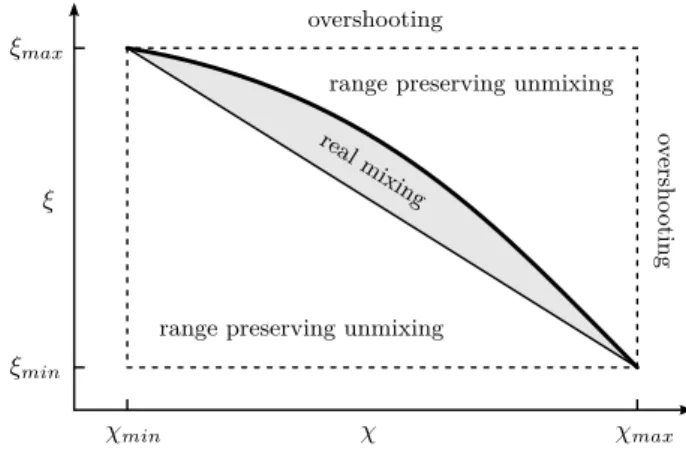
The 11th property above refers to the ability of a scheme to preserve pre-existing functional relations between tracers. Mixing or unmixing can be divided into three categories (see Fig. 1), real mixing, range-preserving unmixing, and over-shooting.
In their native forms, most transport schemes operating on a fixed Eulerian grid (including semi-Lagrangian schemes) will lead to numerical mixing between tracers which, de-pending on the scheme, can fall into any of the three cate-gories. We will term this implicit mixing.
Obviously, range-preserving unmixing and overshooting are unphysical processes, but even real mixing can be so. At a macro spatial scale corresponding to the grid distance in a fluid dynamical model, mixing in nature can be molecu-lar, or a result of turbulence, i.e., deformations of the flow. In geophysical fluid dynamics (GFD) and for typical grid reso-lutions the former is several orders of magnitude smaller than the latter, and, thus, molecular mixing/diffusion is neglected in the governing model equations. To the extent diffusion is parameterized explicitly in GFD models it is therefore sup-posed to represent the mixing associated with unresolved de-formations in the flow. Innon-deformationalflow no mixing should take place and any functional relation between tracers should therefore remain unchanged for inert tracers; i.e., all points in a diagram like that in Fig. 1 will keep their initial positions. Unfortunately, this is not the case for most tradi-tional transport schemes, and therefore they are subject to spurious mixing, even if it belongs to the “real” category. In
ξmin
ξ ξmax
χ
χmin χmax
range preserving unmixing
range preserving unmixing
re alm
ixing overshooting
o
v
e
rs
ho
o
ti
ng
Fig. 1.Illustration of numerical mixing categories. The thick curve is the pre-existing functional relation between tracerξ and tracer χ. Any new relative concentrations(ξk, χk), generated by the
trans-port scheme, can be represented as a point. If the point falls within the shaded convex hull, it is classified as real mixing; if within the dashed rectangle but outside the shaded area it is classified as range-preserving unmixing; and, finally, if outside the dashed rectangle it is classified as overshooting (adopted from Lauritzen and Thuburn, 2012).
the case where the tracers are chemically active, this can po-tentially be a serious problem as spurious chemical reactions are then initiated, or chemical equilibria are displaced.
Note that apart from the initial truncation numerical meth-ods based on orthogonal series expansion functions are the only Eulerian type numerical schemes which do not intro-duce numerical mixing in the case of non-deformational flow. However, generally filters must be introduced in such schemes to prevent e.g. development of negative values, and this introduces numerical mixing also in regions of (quasi-)linear flow.
i.e., spurious accumulation of energy on the shortest resolved scales. The situation is different in pseudo-spectral models where considerably stronger scale selective damping is nec-essary to avoid aliasing.
In conclusion explicit mixing, in terms of filters, diffusion, spectral damping, etc., is needed in both grid point/cell meth-ods and methmeth-ods based on series expansion in order to ensure shape preservation, and in particular positive definiteness, and to control the cascade into smaller scales in a realistic way. In general the combined implicit and explicit mixing will not represent true physical mixing although it may be real in the sense described in Fig. 1.
1.3 The HEL approach
Here we present a numerical methodology, termed the hy-brid Eulerian–Lagrangian (HEL) numerical scheme, which has been designed to fulfill as many as possible of the desired properties mentioned in Sect. 1.1. The aim is to combine the Eulerian and the Lagrangian approaches in such a way that the main problems related to either of these are eliminated or at least reduced. The ideas behind HEL have been inspired by other Lagrangian approaches, in particular that of ATTILA (Atmospheric Tracer Transport In a Lagrangian Atmospheric model) (Reithmeier and Sausen, 2002; Stenke et al., 2008, 2009), which uses a fully Lagrangian scheme for all tracers, including water substances.
Contrary to the problems mentioned in the previous subsection for Eulerian-based schemes, fully Lagrangian schemes are formally exact for the pure advection problem assuming trajectories have been calculated exactly. However, with such schemes, and in general deformational flows, the Lagrangian parcels become irregularly distributed in space and strongly deformed. The irregular distribution is a funda-mental problem for the following reasons:
1. Dynamical tendencies due to non-advective processes generally need to be estimated on a regular grid to en-sure consistency with and between the governing prog-nostic equations.
2. In practice, it is problematic to calculate parameterized physical processes on an irregular grid.
3. There may be sub-domains with no or very few parcels.
The result of an interpolation from mass centers of La-grangian parcels to a regular Eulerian grid will typically, af-ter some time, show a completely unrealistic “spotty” dis-tribution because neighboring parcels originate from quite different positions at the initial time of the integration (see e.g. lower right panel of Fig. 11). In nature, finite size La-grangian parcels typically deform into very long, very thin filaments. A Lagrangian transport scheme aiming at resolv-ing the developresolv-ing shape of individual parcels without any
explicit mixing between neighboring parcels would repre-sent the discrete Lagrangian analogy to the pseudo-spectral method. The aliasing of such a Lagrangian scheme is realized when one interpolates from Lagrangian to physical space, i.e., to a fixed Eulerian grid. To avoid such aliasing one can introduce mixing between parcels. One may think of the dif-ference between a mixed and unmixed Lagrangian scheme as an analogy to the difference between spectral and pseudo-spectral schemes.
In the native form of HEL without parcel mixing the den-sity and, optionally, other prognostic variables are known at all times via a fully Lagrangian as well as a traditional Eu-lerian representation. At each time step a nudging technique is applied where the density information in the downstream translated Lagrangian parcels is used to modify or “repair” an Eulerian-based advection. In this way the non-dispersive, non-diffusive, and shape-preserving advantages of the La-grangian method can be adopted in an otherwise diffusive and/or strongly dispersive Eulerian-based transport scheme. Physical tendency contributions not related to pure advec-tion are most obviously and accurately calculated in Eule-rian space and subsequently interpolated and added to the Lagrangian parcel values. In this way the bulk of the model history is kept in the Lagrangian representation.
With this generic design one is, however, still left with the problem of aliasing in Lagrangian space. To reduce or elimi-nate aliasing a real mixing, described in detail below, is intro-duced in Lagrangian space between neighboring parcels. To mimic the physical nature of the cascade into smaller scales, we let the degree of mixing depend on the local flow defor-mation rate. Not surprisingly, the introduction of such mix-ing turns out to be instrumental for a proper description of the spectral distribution of prognostic variables; however, this is-sue is not covered in the present paper.
Although we are not dealing with chemistry here, it is noted that calculations of chemical reactions are naturally performed in the Lagrangian parcels where it is known that only real mixing takes place.
1.4 Other relevant Lagrangian type numerical schemes
HEL has some similarities to particle in cell (PIC) meth-ods, which have been used extensively in e.g. plasma physics (Tskhakaya et al., 2007). However, one among several fun-damental differences is that in PIC methods the number of Lagrangian parcels far exceeds that of Eulerian grid points/cells, while in HEL these numbers are equal or at least close to the same order of magnitude. The choice of relatively few Lagrangian parcels in HEL was motivated by efficiency considerations since computationally expensive chemical re-actions (not dealt with here) involving up to several hundred chemical tracers should be performed in Lagrangian space.
et al. (2008), ATTILA was implemented in a general circu-lation model to simulate transport of water vapor and cloud water. This was extended in Stenke et al. (2009) to an interac-tively coupled chemistry–climate model version of ATTILA; i.e., water vapor, cloud water, and mixing ratios of all chemi-cal tracers are known for each Lagrangian parcel. ATTILA is able to maintain steep gradients, is mass conserving, numer-ically non-diffusive, and has been used e.g. for studying the climate radiative forcing related to aircraft contrails (Fröm-ming et al., 2011). ATTILA does not handle the “dry dynam-ics” as opposed to HEL; however, besides this the HEL and ATTILA approaches are quite similar when applied for non-dry-dynamical prognostic variables. One difference, though, is that ATTILA on average holds more Lagrangian parcels per Eulerian grid cell than the version of HEL presented here, which on average only has one. More importantly, there are some differences in the way horizontal mixing between neighboring parcels is performed in ATTILA and HEL. For both schemes the degree of mixing depends on the horizon-tal shear deformation rate of the flow; however, in ATTILA this is a simple analytical expression based on Smagorinsky (1963), whereas in HEL the deformation of each parcel is kept as an additional prognostic variable, which is increased each time step in proportion to the shear deformation rate, and attempted to be reduced via realized mixing with neigh-boring parcels.
The approaches in the CLaMS model (McKenna et al., 2002) are less similar than ATTILA to those applied in HEL. The mixing in CLaMS is based on a dynamically adap-tive grid and it becomes acadap-tive in terms of mass exchange between neighboring parcels when the flow deformation is high. A local, in time and space, Lyapunov exponent is used to determine the degree of mixing that takes place, which in practice takes place via generation of new Lagrangian parcels in strongly deformed flow, or merging of clustered Lagrangian parcels. This is one main difference compared to HEL and ATTILA, where Lagrangian parcels survive throughout the integration. In the ATLAS model (Wohlt-mann and Rex, 2009) the flow-dependent mixing method-ology of CLaMS has been modified with emphasis on better performance in lower-resolution model configurations. Also in FPIC (Kaas et al., 1997) an implied mixing takes place via simple birth and merging of particles.
The so-called “trajectory-tracking scheme” introduced in Dong and Wang (2011) and updated in Dong and Wang (2012) has some similarities to HEL. In two-dimensional problems this scheme treats Lagrangian parcels as polygons with a finite number of edges, and with all Lagrangian par-cel polygons spanning exactly the complete integration do-main. The Eulerian space representation is obtained via a first-order conservative remapping so that total mass is con-served in the Lagrangian as well as the Eulerian represen-tation. A “curvature-guard” algorithm is applied in order to maintain an accurate polygon representation in deformation flows. However, this algorithm does not lead to any mixing,
as in HEL, between neighboring Lagrangian parcels. There-fore, in long-term simulations, one should expect problems equivalent to aliasing.
1.5 Overview
The paper is organized as follows: Sect. 2 provides a generic description of the HEL approach, i.e., HEL without any type of mixing between parcels, while Sect. 3 describes how mix-ing between adjacent parcels is achieved. Section 4 presents passive inert transport tests on the sphere. Various traditional and more recently proposed error measures and evaluation statistics are used to demonstrate the performance of HEL in both solid body rotation flow (Sect. 4.1) and in strongly deformational flow (Sects. 4.2 and 4.3). Section 5 deals with some initial attempts to implement HEL as the basis for a dy-namical core in a geophysical fluid dynamics model. In this case the test bed is a shallow water model in plane geome-try. Finally Sects. 6 and 7 discuss the results, including some outlooks for future work, and summarize the basic findings.
2 HEL – passive transport
To introduce the procedure followed in HEL in more detail we first consider the continuity equations for a set ofM trac-ers with densitiesρm:
∂ρm
∂t = −∇ ·(ρmV), m=1, . . . , M, (1)
or alternatively in Lagrangian form,
dlnρm
dt = −∇ ·V, m=1, . . . , M, (2)
whereV is the flow velocity vector. For simplicity we have ignored any sources and sinks, and any diffusion in Eqs. (1) or (2).
It should be noted that other non-FV, yet still mass-conservative, schemes have also been used. For the present work it is of particular relevance to mention the so-called locally mass-conserving semi-Lagrangian method (LMCSL) (Kaas, 2008), which is based on a simple partition of unity principle.
Depending on the chosen order of accuracy any numeri-cal method – Eulerian or semi-Lagrangian type – applied for solving Eqs. (1) or (2) on an Eulerian grid will suffer from some degree of dissipation (or possibly anti-dissipation), some numerical dispersion, and generally, for higher-order schemes, the solution will not be shape preserving.
As mentioned above the main motivation behind the present work is to use a fully Lagrangian forecast, run in parallel, to modify the Eulerian grid forecast in such a way that the above-mentioned disadvantages are reduced or elim-inated. A purely Lagrangian forecast describes the tempo-ral evolution of the densities of individual Lagrangian fluid parcels as they move around. Formally it is straightforward to integrate Eq. (2) for a Lagrangian parcel from timet to some future timet+1t:
lnρ (r(t+1t ), t+1t ))−lnρ (r(t ), t ))
= −
tZ+1t
t
∇·V r(t′), t′dt′
=1t D, (3)
wherer(t )is the position vector of the parcel at timet, andD
represents the average divergence along the trajectory from
r(t )tor(t+1t ). From Eq. (3) one immediately gets
ρ (r(t+1t ), t+1t ))=ρ (r(t ), t ))exp 1t D; (4) i.e., the effect of divergence over the period fromttot+1t
is an expansion/contraction factor:
σ=exp 1t D (5)
multiplied by the original parcel density at timet.
We will now consider the actual numerical discretiza-tion of the prognostic equadiscretiza-tions in Eulerian and Lagrangian space. The Lagrangian parcels are introduced at the initial time, and in the present formulation of HEL they survive throughout the model integration. Also, in the version of HEL presented here, the total number of parcelsP and the number of Eulerian grid cellsKare equal. At the initial time step,n=0, Lagrangian parcel densities,Lρ, are initialized by the corresponding values in Eulerian grid cell centroids; i.e.,
Lρ0
p=Eρk0 Lρ0
m,p=Eρm,k0 , m=1, . . . , M, (6)
wherep, k=1, . . . , P (=K), and mcounts the individual tracers as in Eqs. (1) and (2). In the following we generally
use upper-left superscriptsL andE to indicate Lagrangian and Eulerian space representation, respectively. An upper-right index denotes the time step. A list of all prognostic variables in HEL to be described below can be found in Ap-pendix A.
Assume some numerical scheme has been used to solve Eqs. (1) or (2) in the Eulerian grid cell representation, and let
Eρ˜n+1
k Eρ˜n+1
m,k, m=1, . . . , M (7)
denote the forecast in Eulerian grid cellsk=1, . . . , Kat time step n+1. In general we use the notation (˜·)to represent some provisional approximate value. This is also the case here whereρ˜ indicates that the forecast at time stepn+1 is only a provisional Eulerian space forecast to be modified by densities in the Lagrangian representation.
Letting parcels follow downstream trajectories from time stepnton+1 estimated from the actual velocity components in the Eulerian grid, one obtains an approximate Lagrangian solution to the pure advection problem. However, in a gen-eral divergent flow the parcel volume density will of course undergo changes. According to Eqs. (4) and (5) the effect of divergence for parcelpfrom time stepnton+1 can simply be modeled as
Lρn+1
p =Lσ
n+1/2
p Lρpn, (8)
where superscript n+1/2 indicates that the expan-sion/contraction factor represents the effect of divergence from time stepnton+1. In practiceσn+1/2is determined in Eulerian space from the provisional Eulerian space forecast of the “dry air” density,Eρ˜n+1, i.e., including the effect of divergence, and from a corresponding purely advective fore-cast, i.e., not including the effect of divergence, which we termE,advρn+1:
Eσn+1/2= Eρ˜
n+1
k
E,advρn+1, k=1, . . . , K. (9) For cell-integrated FV and the LMCSL schemes applied in the present paper the calculation ofEσn+1/2is straightfor-ward since estimation ofE,advρn+1 is an inherent part of these schemes.
Once new downstream parcel positionsLrn+1 have been found, Lσn+1/2 can be obtained via interpolation from
Eσn+1/2. The parcel forecast for parcelp, including diver-gence, then simply becomes
Lρn+1
p =
Lσn+1/2
p Lρpn
Lρn+1
m,p=Lσ
n+1/2
p Lρm,pn , m=1, . . . , M. (10)
It is important to note that in a dynamical model, in or-der to prevent numerical instabilities related to fast modes, e.g. gravity waves,Eσpn+1/2must be based on divergence
The modification of the Eulerian densities using the parcel densities is done by first interpolating the irregularly spaced parcel densities to the Eulerian grid obtaining certain Eule-rian space target values,ET andETm, m=1, . . . , M, and then nudging the original Eulerian-based forecast towards these values under the constraints of mass conservation and shape preservation (see details in Sect. 2.6).
A generic recipe in an atmospheric multi-tracer applica-tion of HEL, not yet considering the mixing, can be summa-rized as follows at a given time stepn(here omitting indices for Eulerian grid cells,k, and Lagrangian parcels,p):
1. Perform a conventional, preferably inherently mass-conserving, Eulerian or semi-Lagrangian time step of total dry density, Eρ˜n+1, valid on an Eulerian grid. This is termed theprovisional forecast.
2. Perform a corresponding purely advective time step in Eulerian spaceE,advρn+1 of the dry density, and use this to calculate the divergent multiplication fac-tor,Eσn+1/2=Eρ˜n+1/E,advρn+1.
3. For all tracers, m=1, . . . , M, perform a provisional Eulerian space forecast,Eρ˜n+1
m .
4. Perform a pure downstream displacement of the irreg-ularly spaced Lagrangian parcels; i.e., calculate down-stream trajectories and reposition each parcel fromLrn
toLrn+1.
5. InterpolateEσn+1/2from the Eulerian grid cells to the positionsLrn+1resulting in valuesLσn+1/2. Then cal-culate the new parcel densities for both the dry air and all the tracers, including the effect of divergence:
Lρn+1=Lσn+1/2·Lρn, andLρn+1
m =Lσn+1/2·Lρmn,
m=1, . . . , M.
6. InterpolateLρn+1from the Lagrangian grid to obtain the target values,ET, in the Eulerian grid. In Eulerian
grid cells with no nearby Lagrangian parcelsETn+1is set equal toEρ˜n+1from step 1; see details in Sect. 2.5. 7. As step 6 but for all tracersm=1, . . . , M.
8. Nudge Eρ˜n+1 towards ETn+1 under constraints of mass conservation and shape preservation for the den-sity; see details in Sect. 2.6. The result is the final HEL forecast,Eρn+1, for the dry air in Eulerian space. 9. As step 8 but for all tracers m=1, . . . , M. However,
now the constraints are mass conservation and shape preservation for tracermixingratios.
2.1 The underlying numerical scheme
As outlined above, some numerically stable scheme must be chosen in order to obtain the provisional forecast in Eule-rian grid space. For applications in HEL it would be rea-sonable to use a semi-Lagrangian type scheme since trajec-tory calculations can be partly re-used for estimation of the
downstream parcel trajectories; also, it would then be possi-ble to take long steps not subject to classical CFL conditions for advective processes. Therefore relevant schemes include, e.g., flux-based multidimensional schemes such as Lin and Rood (1996) and Leonard et al. (1996), the Departure area Cell-Integrated Semi-Lagrangian (DCISL) scheme (Machen-hauer and Olk, 1997), the Conservative Semi-LAgrangian Multi-tracer transport scheme (CSLAM) (Lauritzen et al., 2010), the Semi-Lagrangian Inherently Conserving and Ef-ficient scheme (SLICE) (Zerroukat et al., 2002), or the Lo-cally Mass-Conserving Semi-Lagrangian scheme (LMCSL) (Kaas, 2008).
Note, however, that any mass-conserving scheme for solv-ing continuity equations can in principle be used as the un-derlying scheme for HEL. In fact, relaxing the mass con-servation property, any consistent numerical scheme can be used.
In the present paper we have tested the use of first- and third-order versions of the CSLAM and LMCSL schemes to obtain the first guess forecast in Eulerian space.
2.2 Estimation of trajectories
The downstream displacement of parcel locations obviously is an essential component in HEL. In simple numerical tests such trajectories can be calculated analytically, or, as in dy-namical models, they can be calculated via an iterative pro-cedure, which is equivalent to that used in traditional semi-Lagrangian models for estimating the upstream departure points/cells. In the present applications we have generally used analytical or approximate analytical trajectories for ide-alized numerical tests, and iteratively estimated trajectories in dynamical model implementations. This is described fur-ther in Sects. 4.1, 4.2, and 5.1.1.
2.3 Update of the parcel volumes
Each Lagrangian parcel represents a certain volumeLV of the fluid which, at the initial time step, is simply initialized as the volume represented by the volume of the relevant Eu-lerian grid cell.
OnceLρn+1has been calculated one can update the vol-ume of each parcel. Omitting the upper index “L” the parcel volumeVpn+1at time stepn+1 is determined diagnostically by the constraint that, in the absence of mixing, the total mass of each Lagrangian parcel is conserved, i.e.,
Vpn+1ρpn+1=Vpnρpn (11) whereby
Vpn+1=Vpn ρ
n p
ρpn+1
= V
n p
σpn+1/2
using Eq. (10).
The volume of the parcels is a necessary ingredient for mixing between neighboring parcels (Sect. 3).
2.4 Interpolations from Eulerian to Lagrangian representation
Interpolations between the Eulerian and Lagrangian repre-sentations are required as part of the HEL scheme. For ex-ample, as explained above, it is necessary to interpolateσ to the Lagrangian representation. Similarly, when HEL is used in a dynamical model, tendencies related to other physical processes must be interpolated.
In the present formulation of HEL all interpolations from the Eulerian grid cells to the Lagrangian parcel locations are fourth-order Lagrange polynomial interpolations.
2.5 Target values
Provisional target values,ET˜n+1, for the Eulerian space dry air density can be obtained when Eρ˜n+1 and Lρn+1 have been calculated. The provisional target value in Eulerian grid cell k is composed as a weighted sum of the provisional Eulerian-based forecast,Eρ˜kn+1, and a parcel-based estimate
Rk:
ET˜n+1
k =
w1Eρ˜kn+1+w2Rk
w1+w2
, (13)
whereRkis defined as
Rk= 1
Wk P
X
p=1
wp,kEρˆp,kn+1 with Wk= P
X
p=1
wp,k, (14)
wherewp,kis a simple bi-linear interpolation weight given to
an estimate of the densityEρˆnp,k+1in Eulerian grid cellkwhich is based on the density at the location of parcel numberp:
Eρˆn+1
p,k =
Lρn+1
p +(Lrnp+1−rk)·gp,k. (15)
gp,kis a second-order numerical approximation to the
gradi-ent∇ Eρ˜n+1at the location 0.5(Lrn+1
p +rk), andrkis the
position vector of thekth Eulerian grid cell.
The weightsw1andw2in Eq. (13) are determined as fol-lows:
w1=max[w0, (1−Hk)Wk]
w2=HkWk, (16)
wherew0 is a small positive number, andHk is a measure
of the homogeneity of the distribution of Lagrangian parcels around the Eulerian cellk. Here we have used the following estimate ofHk:
Hk=
2×min[Wl]
max[Wl] +min[Wl]
l∈Lk, (17)
k
4k
2k
1k
3n
+1
n
Fig. 2.Traditional upstream semi-Lagrangian departure point.
whereLk is a subset of Eulerian cells includingk and its
nearest eight surrounding neighbors (for a regular grid as used here). In Eq. (16) the maximization ofw1is introduced to ensure that the target values are always well defined. The value ofw0has, somewhat arbitrarily, been set to 10−5; i.e., in the target values estimated from Eq. (13) there will always be some weight on the Eulerian-based forecast. In general this weight is small but in the special case whereWk=0,
i.e., where there are no neighboring parcels at all, the target value will simply be equal to the provisional Eulerian fore-cast.
In practice the calculations of Rk and Wk are not
per-formed as sums over all parcels as indicated in Eq. (14) since this would be very inefficient numerically because it is known that only four of the parcel weights,wp,k, for a given
parcelpare different from zero. InsteadRk andWk are
cal-culated in a single loop over all parcels where information is distributed (summed) to the neighboring four Eulerian cells, followed by a second loop where the result is divided by the sum of weights for each cell.
Provisional target values for the tracers ET˜mn+1, m=
1, . . . , Mare obtained via the same technique as outlined for the dry air, i.e.,ET˜n+1above. I.e., all weights are the same.
To obtain an Eulerian space forecast, which is shape pre-serving and compatible we must identify minimum and max-imum permitted mixing ratios,q−andq+, respectively, for each tracermin each Eulerian grid cell. The mixing ratio for a tracer mis defined as qm=ρm/ρ, implying that we can
always deduce mixing ratios in both the Eulerian and La-grangian representation whenρmandρ are known, and we
can always convert a mixing ratioqm back to volume
Thus the provisional minimum and maximum mixing ra-tios for tracermbecome
Eq˜−
m,k=min[Eq n m,ki] Eq˜+
m,k=max[Eqm,kn i]
, i=1, . . . ,4. (18)
The final limits are obtained by using additional information from mixing ratios in theQparcelspi, i=1, . . . , Qthat have
Euclidian distance to the Eulerian cellkat time leveln+1, which is less than 1.5 grid distances:
Eq−
m,k=min[
Eq˜ m,k,Lq
n+1
m,pi] Eq+
m,k=max[Eq˜m,k,Lq n+1
m,pi]
, i=1, . . . , Q. (19)
Once the Eulerian space forecast for dry air densityEρhas been obtained, the minimum and maximum permitted val-ues of volume density for tracerm=1, . . . , Mcan easily be obtained:
Eρ−
m,k=
Eq−
m,k· Eρ
k, (20)
Eρ+
m,k=
Eq+
m,k· Eρ
k. (21)
2.6 Nudging of first guess towards target values
After the (shape-preserving) target values have been calcu-lated, the provisional, “first guess”, Eulerian forecast can be corrected. The correction, or nudging, is done in two steps. First we calculate the total mass,M=PKk=1Eρ
k·EVk, and
the total mass of the target values,MT =PKk=1ETk·EVk, as
well as the discrepancy,1M=MT −M, between the two. This will lead to three different possibilities:
1M <0: Mass of target field is too small.
1M=0: Mass of target field is correct.
1M >0: Mass of target field is too large.
In the (extremely unlikely) event that the mass of the tar-get field is exact (1M=0), the Eulerian field is simply re-placed by the target field. In the two remaining possibilities the target field has to be modified to ensure mass conserva-tion. If the mass of the target field is less that the actual mass (1M <0), we calculate the maximum possible mass of the field, i.e.,M+=PKk=1ρk+·EV
k, where shape preservation
is still fulfilled. The target field and the maximum field can then be combined to produce a final corrected Eulerian field, which is both mass conserving and shape preserving.
w+= 1M
M+−MT (22)
Eρ
k=(1−w+)·ETk+w+·Eρ
+
k. (23)
This is always possible as M+≥M. The procedure is the same if the mass of the target field is too large; then
the target field is weighed with the minimum mass field,
M−=PKk=1ρk−·EVk, to acquire mass conservation.
w−= 1M
MT −M− (24)
Eρ
k=(1−w−)·ETk+w−·Eρ
−
k. (25)
The procedure is then repeated for all tracersm=1, . . . , M. The nudging employed in the current version is global, but since all chemistry is calculated in the Lagrangian parcels, it will not introduce errors due to the inevitable numerical mix-ing in the Eulerian domain. A local nudgmix-ing method has also been tested, but it leads to somewhat poorer – and in prac-tice less localized – results, as the nudging method’s ability to correct the Eulerian values will be lessened by hard local-ity constraints. The traditional concerns when using global methods, i.e., mass redistribution and unphysical mixing, is fully controlled by the correct values being preserved in the Lagrangian parcels, meaning that HEL is very “local”.
3 Mixing between parcels
As discussed in Sect. 1 densities/mixing ratios or other in-variants will generally develop into thin filaments as part of the cascade into smaller and smaller scales in geophysical deformational flows. At some point a model at given res-olution cannot represent the spatial scale of the filaments, and explicit horizontal diffusion may therefore be required to prevent spectral blocking. Considered in discrete Lagrangian space, i.e., a model, the analogue to spectral blocking is re-alized as a gradual development into unrealistically large differences between densities/mixing ratios in neighboring parcels.
An example of this is presented below in Sect. 5. There-fore, due to their non-dissipative nature, explicit mixing must be introduced in Lagrangian models. We introduce a direc-tionally biased mixing as an a posteriori operation applied each time step after the generic HEL forecast, described above, has been obtained.
In the present paper we only consider two-dimensional flow. In this case the degree of mixing between neighbor-ing parcels is based on a modified instantaneous and local two-dimensional rate of deformation:
Dn=max
0,
s∂vn
∂x + ∂un ∂y 2 + ∂un ∂x − ∂vn ∂y 2 − ∂un ∂x + ∂vn ∂y , (26)
Time step n
a
na
n
a
n+1
a
n+1True asymptotic
shear dilatation axi
s
a
n+1a
n+1Time step n+1 Normalize at time step n+1
True asymp totic
shear d
ilatation axis
True asymptotic
shear dilatation axi
s
Δ Δ
Δ Δ
Pa
P P
P
Pa Pa
P
a
P P
P
Δ
Δ
Δ
Fig. 3.Downstream advection of two different Lagrangian parcels and their auxiliary parcels in a pure shear flow. For each parcelP and Pa denote, respectively, its position and the position of the auxiliary parcel. The associated auxiliary vectors are marked black and gray, respectively, to distinguish between the two parcels. In this example the (true) asymptotic/Lagrangian dilatation axis, indicated with dashed lines, is the same all over the small domain shown, although its direction rotates clockwise from time stepnto time stepn+1. Note that it is the relative movements between parcels and auxiliary parcels that are relevant. After several time steps the auxiliary vectors will align approximately with the true asymptotic dilatation axis.
should not lead to excessive damping when the scheme is ap-plied to the full mass field in a dynamical model. Not intro-ducing such a modification would tend to damp dynamically important gravity waves.
The calculation ofD is estimated in Eulerian space via
centered, i.e., second-order accurate, differences. The ex-pression in Eq. (26) is only valid in Cartesian geometry. Therefore, in the applications on the sphere presented below, metric factors have been applied.
In addition to the prognostic variables discussed above a set of three prognostic variables are introduced in Lagrangian space (only) in order to perform the mixing. For each La-grangian parcelp these include the actual parcel deforma-tion,Lδp, and the two coordinates of a position vector,Lrpa,
of a passive auxiliary Lagrangian parcel,Lpa, that is used to identify the asymptotic dilatation axis for shear, i.e., the direction of “long-term” parcel stretching due to shear con-sidered in a Lagrangian sense; see e.g. Cohen and Schultz (2005).
For each parcelp its deformation is initialized to zero at the first time step:Lδ0p=0, and it is updated as part of the mixing procedure described below. The location of the aux-iliary parcelpafor main parcelpis initialized one grid dis-tance,1, away frompin an arbitrary direction on the inte-gration plane. At each time step the auxiliary parcel is trans-lated downstream using the same trajectory algorithm as for the main parcels.
The mixing operates as follows:
1. Once the modified deformation rate,Dn, has been de-termined in Eulerian space at a given time step, it can be interpolated to the parcel positions enabling calcu-lation of new provisional parcel deformations:
Lδ˜n+1
p =Lδpn+1tLDnp. (27)
2. Omitting for simplicity the Lagrangian and parcel in-dicesLandp, and the time indexn+1, letr˜adenote the pure downstream position vector of the auxiliary parcel for a main parcel, which has downstream posi-tion vectorr. The final downstream position vectorra of the auxiliary parcel is then defined as
ra=r+1 ˜ ra−r ||˜ra−r| |
; (28)
i.e., the distance between a parcel and its auxiliary par-cel is simply normalized to one grid distance. Two ex-amples of the identification of theavector are shown in Fig. 3. No formal proof is given here that the vec-tors ra will actually converge toward the Lagrangian shear dilatation axes. Since the additional parcelsaare initialized randomly, a certain time will elapse from the model initial state until realistic dilatation axes are identified for each parcel. However this time is propor-tional to the deformation rate of the flow, and there-fore, when the deformation rate is large, the dilatation axes is also quickly approached. Obviously if the flow is linear, i.e., no mixing is needed, then the dilatation axes of the model parcels maintain their initial random orientations.
3. For each parcel,p, letµp,krepresent a fraction of the
parcel volume,LVp, which is assigned to a
neighbor-ing Eulerian grid cell centroidk.µp,kis defined as
µp,k=0.25 min
h
1,Lδ˜np+1
i
exp(−κdp,k2 ), (29) where dp,k is the distance in units of grid distances
Asymptotic (Lagrangian) d
ilatation axis
Δ
Δ
Δt⋅D⋅ Δ
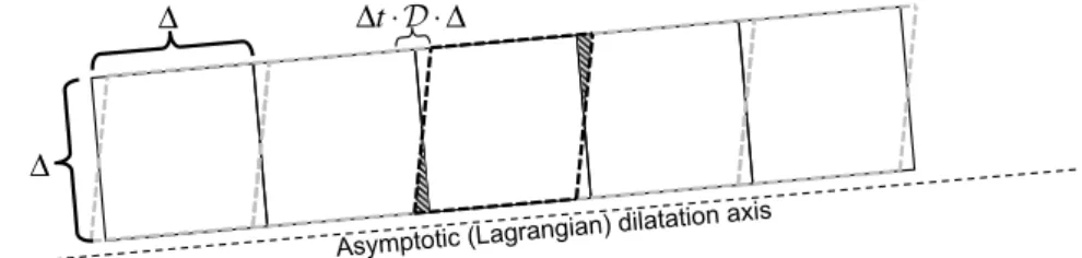
Fig. 4.This figure describes why we use a factor of 0.25 between the deformation within one time step1t·Dand the fraction of the parcel area12that should be mixed. The underlying assumption is that the deformation is mainly due to shear, and the figure shows how cells are then deformed within one time step from regular squares into irregular parallelograms with the same area (assuming zero divergence). In order to re-shape a cell into squares the mass in the two shaded triangles must be given off via interpolations to the neighboring cells. The factor comes because the sum of the triangular areas is 0.251t·D12.
dp,k=0.5, then the exponential factor in Eq. (29)
be-comes about 0.1; i.e., only grid cells close to theps’ dilation axis are assigned an appreciable fraction of volume. For all Eulerian pointskwith distances top
larger than1,µp,kis set to zero. I.e., in a regular grid
µp,kis only different from zero for a maximum of four
individual values of k. It is ensured that the sum of these four weights does not exceed unity. The factor “0.25” is obtained from geometrical considerations of the relationship between deformation rate and the frac-tion of the parcel volume which should be mixed with neighboring parcels – see Fig. 4.
4. Once µp,k is calculated, a total mass contribution,
µp,kLρm,pVp, for each tracermis transferred from the
Lagrangian parcelp to Eulerian grid cellk. In other words the average density of mass contributions from all parcels “neighboring”kis
ρm,k= P
pµp,kLρm,pVp
P
pµp,kVp
, (30)
where it is noted that µp,k represents elements in a
sparse matrix with non-zero contributions from no or only a few parcels.
5. Now the mixing can be realized by transferring the mixed densities in the Eulerian cells back to the La-grangian parcels. For parcelpthe final mixed density
Lρ
m,pbecomes Lρ
m,p=(1−µp,k)u,Lρm,p+µp,kρm,k, (31)
where we have formally used the notationu,Lρm,p to indicate the unmixed forecasted density in parcelp re-sulting from the generic HEL recipe.
Note that not only tracers are mixed using Eq. (31). To ensure full consistence between prognostic variables also the dry air is mixed.
It can easily be shown that the total parcel mass for each tracer and for the complete “dry parcel
mass of the atmosphere” are conserved when applying Eq. (31).
6. Based on the amount of actual mixing,Mp, that has
taken place for parcel pvia the above operations the final parcel deformation is calculated. The actual mix-ing, not including trivial mixing of parcels with them-selves, is
Mp=X
k
µp,k
P
p′wp′,kVp′−µp,kVp
P
p′wp′,kVp′
, (32)
where it is again noted that for regular grids the sum overkonly includes four grid cells surrounding parcel
p. The parcel deformation is finally reduced according to the degree of mixing that has actually taken place:
Lδn+1
p =Lδ˜pn+1(1−4Mp), (33)
where the factor of “4” is a constant determining how muchLδp is reduced per unit change in relative area.
This factor is obtained from the same geometrical con-siderations mentioned above (see Fig. 4) of the rela-tionship between deformation rate and the fraction of the parcel volume which is actually mixed with neigh-boring parcels. Note that the factor of 0.25 in Eq. (29) ensures thatLδpn+1cannot be less than zero.
Most computational operations in the above list are common for all tracers, and therefore, in multi-tracer applications, the total number of operations is limited.
the problem of numerical mixing and unmixing is eliminated. It is noted that the introduction of a flow-dependent mixing based on the degree of deformation is not new. Sadourny and Maynard (1997) introduced a horizontal diffusion which was dependent on the magnitude of the deformation rate of the flow, and later Váˇna et al. (2008) used a similar approach to obtain a flow dependent degree of mixing in a semi-Lagrangian model. Also ATTILA (Stenke et al., 2009) and CLaMS (Chemical Lagrangian Model of the Stratosphere) (McKenna et al., 2002) employ mixing depending on hori-zontal flow deformation rate.
4 Passive tracer numerical simulations on a cubed sphere
To validate HEL we perform inert passive tracer transport on the sphere driven by both solid body rotation and two types of deformational flow.
For the passive transport tests presented here the underly-ing Eulerian-based scheme required in HEL is a first-order (i.e., shape preserving by definition) version of CSLAM (Lauritzen et al., 2010). Where necessary this is referred to as CSLAM-1st. The performance of HEL is compared to that of a third-order accurate version of CSLAM in combination with a simple shape-preserving filter (Lauritzen et al., 2010), referred to as CSLAM-M.
In the tests shown here both HEL and CSLAM have been implemented on a so-called cubed sphere grid – see Lau-ritzen et al. (2010) for details.
4.1 Solid body rotation
In standard solid body rotation tests on the sphere a certain spatial distribution returns to its original position after one or more rotations. In this case HEL should perform with high accuracy since the parcels end up in exactly the same grid cell centroids they were initialized in, and no mixing takes place because the deformation rate of this flow is zero. Thus the target values will be almost exactly equal to their initial value, except for the small weight factorw0(see Eq. 16). This again implies that the final HEL forecast should be almost exactly equal to the corresponding analytic solution since global nudging is used.
The test example we present here is the solid body advec-tion of a cosine bell with radiusRc=R/3, whereRis the ra-dius of the Earth. The angle of rotation isπ/4 relative to the Earth rotation axis; i.e., the bell passes over the edges of the cubed sphere. One full revolution is completed in 576 time steps of 1800 s each. These settings are identical to those in Putman and Lin (2007).
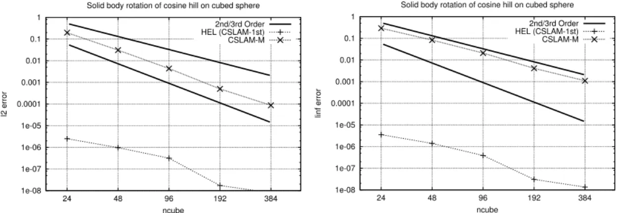
To validate the results obtained with this simple setup we use the traditional l2 andl∞ error norms. Results in terms of l2 andl∞ after one revolution are plotted in Fig. 5. As expected the HEL is very accurate due to the low value of
thew0weight. Thel2andl∞convergence rates for CSLAM-M are 2.82 and 2.04, respectively, while they are 2.24 and 2.16 for HEL. It is noted that the convergence rate for HEL increases significantly if a fixed Courant number is used in such tests (not shown) because this implies that, as the time step decreases, the weight per time unit on the parcels in-creases relative to that on the underlying Eulerian-based fore-cast. While the accuracy increases the shorter the time step in HEL, the opposite is generally the case in semi-Lagrangian models such as CSLAM because the number of remappings increases when the time step is reduced.
The temporal growth of error in HEL and in CSLAM-M are quite different: running over several revolutions the er-ror norms continue to grow in CSLAM-M, although slowly, while in HEL the error norms do not grow with time, as one should also expect from the way HEL is designed.
4.2 Deformational flow tests
For the deformation flow tests we have used the two types of analytic flow fields, the density shapes, and the validation diagnostics suggested in Lauritzen et al. (2012), and used in a model intercomparison (Lauritzen et al., 2013). For the di-agnostics this means that, in addition to thel2andl∞error norms and related convergence rates used for the simple solid body rotation tests above, we have calculated an additional set of diagnostics, briefly described below.
The two analytical flow fields used have originally been proposed by Nair and Lauritzen (2010), and they include a non-divergent as well as a divergent flow. In both cases the Lagrangian parcels follow relatively complex trajectories, and the flow is composed of a deformational deformation component, which is different in the two cases, and an over-laid translational flow. The translational part is designed to perform exactly one rotation around the sphere (along equa-tor) during the entire simulation. After a half complete pe-riod of simulation the deformational flow component goes to zero, and this part of the flow is then reversed so that the final exact solution equals the initial condition. Half way through the simulation, at the time when the deformational flow com-ponent goes to zero and starts to reverse, the initial distribu-tions are deformed into thin filaments, particularly for the non-divergent flow.
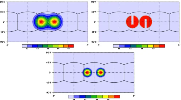
Three initial, i.e.,t=0, distributions consisting of two iso-lated Gaussian hills, two slotted cylinders, and two cosine hills are shown in Fig. 6. Details for these distributions are described in Lauritzen et al. (2012).
As an example Fig. 7 shows the result of simulations att=
1e-08 1e-07 1e-06 1e-05 0.0001 0.001 0.01 0.1 1
24 48 96 192 384
l2 error
ncube
Solid body rotation of cosine hill on cubed sphere
2nd/3rd Order HEL (CSLAM-1st) CSLAM-M
1e-08 1e-07 1e-06 1e-05 0.0001 0.001 0.01 0.1 1
24 48 96 192 384
linf error
ncube
Solid body rotation of cosine hill on cubed sphere
2nd/3rd Order HEL (CSLAM-1st) CSLAM-M
Fig. 5.Test of convergence for linear advection on cubed sphere using error normsl2(left) andl∞(right). ncube refers to the number of grid cells in each direction on each of the 6 faces of the cubed sphere; i.e., ncube=24 corresponds to an equatorial angular grid distance of 2π/(4×24)=0.065 radians.
For illustrative purposes Fig. 7 also includes the result of a simulation without any parcel mixing, and where the param-eterHk deliberately has been set to unity. In this case, as can
be seen, the distribution at timet=T /2 becomes unrealis-tic since the initial distribution has been cut into small parts (represented by the individual parcels). However, as expected since time is reversed, the final distribution in this aliased model setup is very close to the analytic solution. It is only small errors in the parcel trajectories, and the fact thatw0is different from zero, that prevents the final field from being equal to the analytical solution.
Using the non-divergent flow, basic error norms l2 and
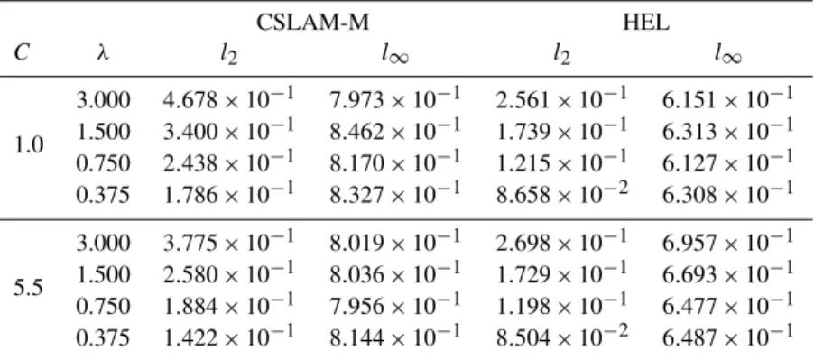
l∞ for CSLAM-M and HEL, and two maximum Courant numbers (1.0 and 5.5), are listed in Tables 1, 2, and 3 for each of the three initial distributions. In general one can con-clude that HEL is very accurate at low resolution for the smoother distributions, i.e., the Gaussian and cosine hills, whereas CSLAM-M and HEL are comparable at the high Courant number and at the two finest resolutions. Another feature is that, as compared to CSLAM-M, HEL is less sen-sitive to the maximum Courant number. This is because HEL is influenced much less by the number of semi-Lagrangian remappings needed to finalize each simulation than CSLAM-M.
The convergence rates for each of the three initial distri-butions and for the two Courant numbers are listed in Ta-ble 4. In general CSLAM-M converges faster than HEL at high Courant number for the smooth distributions, while the difference is small for the rough slotted cylinder distribution where the convergence rates in any case are low. The conver-gence rates are comparable in the low Courant number cases.
4.2.1 “Minimal” resolution
Numerical schemes may be constructed to converge fast – at least for smooth distributions. However, as pointed out by Lauritzen et al. (2012) increases in resolution are often
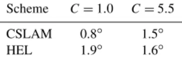
computationally expensive, and therefore it is of interest to identify some kind of measure of absolute accuracy for a nu-merical scheme. A diagnostic designed for this is the “min-imal” resolution needed to obtain a certain accuracy for a specific problem. Following the specifications in Lauritzen et al. (2012) we have calculated the minimal resolution as the resolution required to obtain anl2error norm for the co-sine bell distribution that is less than 0.033. In the specifica-tions (Lauritzen et al., 2012) the result should be obtained for an unlimited scheme, i.e., no shape-preserving limiter should be applied, e.g. on CSLAM, in this case. Minimal resolutions for CSLAM and HEL are listed in Table 5.
The minimal resolution for HEL is coarser than that for CSLAM, particularly for a maximum Courant number of 1. We therefore conclude that the effective resolution for HEL is higher than for CSLAM.
The minimal resolution for HEL is controlled by the strength of the mixing between parcels. If HEL is run without any parcel mixing the minimal resolution goes to infinity in the sense that the numerical solution becomes almost exactly equal to the analytic solution at any resolution, of course de-pending on the weightw0.
4.2.2 Filament diagnostics
The filament preservation diagnostic,lf, describes the trans-port scheme’s ability to preserve thin filaments or gradients in the concentrations.lfis defined as
lf=
100.0·A(τ,tA(τ,t )=0) ,ifA(τ, t=0)6=0
0.0 ,else , (34)
Fig. 6.Initial (and final analytic) distributions for deformational test cases: Gaussian hills (upper-left panel), slotted cylinders (upper-right panel), and cosine hills (lower panel).
Table 1.Statistics for the Gaussian hill problem. The columns show maximum Courant number (C), equatorial resolution in degrees (1λ), and the error normsl2andl∞, respectively, for both CSLAM-M and HEL.
CSLAM-M HEL
C λ l2 l∞ l2 l∞
1.0
3.000 2.422×10⁻¹ 3.434×10⁻¹ 4.593×10⁻² 6.934×10⁻² 1.500 7.606×10⁻² 1.576×10⁻¹ 1.397×10⁻² 3.284×10⁻² 0.750 1.376×10⁻² 5.475×10⁻² 4.499×10⁻³ 1.431×10⁻² 0.375 2.592×10⁻³ 1.850×10⁻² 1.661×10⁻³ 6.989×10⁻³
5.5
3.000 9.953×10⁻² 1.415×10⁻¹ 6.837×10⁻² 1.021×10⁻¹ 1.500 1.990×10⁻² 5.084×10⁻² 1.889×10⁻² 2.814×10⁻² 0.750 3.112×10⁻³ 1.767×10⁻² 5.474×10⁻³ 1.570×10⁻² 0.375 5.371×10⁻⁴ 5.978×10⁻³ 1.825×10⁻³ 6.990×10⁻³
Table 2.As Table 1 but for the slotted cylinder problem.
CSLAM-M HEL
C λ l2 l∞ l2 l∞
1.0
3.000 4.678×10⁻¹ 7.973×10⁻¹ 2.561×10⁻¹ 6.151×10⁻¹ 1.500 3.400×10⁻¹ 8.462×10⁻¹ 1.739×10⁻¹ 6.313×10⁻¹ 0.750 2.438×10⁻¹ 8.170×10⁻¹ 1.215×10⁻¹ 6.127×10⁻¹ 0.375 1.786×10⁻¹ 8.327×10⁻¹ 8.658×10⁻² 6.308×10⁻¹
5.5
3.000 3.775×10⁻¹ 8.019×10⁻¹ 2.698×10⁻¹ 6.957×10⁻¹ 1.500 2.580×10⁻¹ 8.036×10⁻¹ 1.729×10⁻¹ 6.693×10⁻¹ 0.750 1.884×10⁻¹ 7.956×10⁻¹ 1.198×10⁻¹ 6.477×10⁻¹ 0.375 1.422×10⁻¹ 8.144×10⁻¹ 8.504×10⁻² 6.487×10⁻¹
(0.10, . . . ,0.95). The values oflfare expected to increase for low values ofτ and decrease for high values ofτ due to nu-merical diffusion. Atτ =0.1 the value oflf should be 100, since the area with the background concentration should not be increased during the simulation.
The lf values for CSLAM-M and HEL are presented in Fig. 8 for simulations with maximum Courant numbers 1 and 5.5. As expected CSLAM-M is more diffusive; i.e., it maintains filaments less well, at maximum Courant num-ber 1 as opposed to 5.5. This is because more remappings are required at the lower Courant number. The HEL val-ues are calculated for both Eulerian and parcel, i.e., La-grangian, representations. It can be concluded from Fig. 8 that at timet=T /2 of the simulation the Eulerian represen-tation of HEL is generally more diffusive than CSLAM-M for the high maximum Courant number although the high-est functional values are maintained to a higher degree than for CSLAM-M. This is because a relatively large weight,
w1, in Eq. (13) is given to the provisional first-order Eu-lerian forecast,Eρ˜n+1, due to the highly inhomogeneously spaced parcels at this time. The Eulerian HEL representation does not change significantly with Courant number and is generally better at preserving the maximum values than the CSLAM-M. Therefore the low Courant number CSLAM-M
is more diffusive than the corresponding Eulerian HEL repre-sentation. The Lagrangianlfvalues are generally much closer to 100 than the corresponding CSLAM-M and Eulerian HEL representations, and there is almost no dependency on the Courant number. The last observation is completely as ex-pected since the parcel mixing takes place at the same time interval in the two cases. It is noted (not shown) that thelf values are quite insensitive to the mixing frequency between Lagrangian parcels. In a more general application, using non-analytic trajectories, there could in theory be some spatial overlapping between parcels. However, such overlaps cannot be quantified due to deformation of the Lagrangian parcels into filaments, and HEL does not include information about their exact shape. The total area, however, is conserved.
Table 3. As Table 1 but for the cosine hill problem.
CSLAM-M HEL
C λ l2 l∞ l2 l∞
1.0
3.000 3.898×10⁻¹ 5.268×10⁻¹ 7.246×10⁻² 9.585×10⁻² 1.500 1.625×10⁻¹ 2.903×10⁻¹ 2.169×10⁻² 3.025×10⁻² 0.750 2.844×10⁻² 9.827×10⁻² 6.244×10⁻³ 1.119×10⁻² 0.375 6.397×10⁻³ 3.319×10⁻² 1.998×10⁻³ 5.437×10⁻³
5.5
3.000 2.036×10⁻¹ 2.684×10⁻¹ 9.807×10⁻² 1.502×10⁻¹ 1.500 4.330×10⁻² 8.907×10⁻² 2.829×10⁻² 4.533×10⁻² 0.750 6.674×10⁻³ 3.063×10⁻² 7.673×10⁻³ 1.336×10⁻² 0.375 1.357×10⁻³ 1.047×10⁻² 2.241×10⁻³ 5.579×10⁻³
Table 4.l2andl∞convergence rates calculated from the error norms listed in Tables 1, 2, and 3. The second column gives the initial spatial distribution with “GH” indicating Gaussian hill, “SL” slotted cylinder, and “CH” cosine hill, while the convergence rates are listed in columns three through six.
Scheme Initial distr. l2,C=1.0 l∞,C=1.0 l2,C=5.5 l∞,C=5.5
CSLAM-M GH 2.21 1.42 2.53 1.52
HEL GH 1.60 1.11 1.75 1.24
CSLAM-M SL 0.46 0.01 0.47 0.01
HEL SL 0.52 0.01 0.55 0.04
CSLAM-M CH 1.68 1.14 2.44 1.56
HEL CH 1.77 1.55 1.82 1.60
Table 5. “Minimal” resolution required to obtain anl2error norm less than 0.033 for the cosine hill problem in the non-divergent de-formation flow. The columns include scheme and Courant number.
Scheme C=1.0 C=5.5
CSLAM 0.8◦ 1.5◦
HEL 1.9◦ 1.6◦
pseudo-spectral models. So, although we know that explicit mixing must be introduced in some undiffusive models for purely physical reasons, we do not know exactly how much mixing is required. I.e., the optimal lf values are, unfortu-nately, also unknown. The fundamental idea behind the par-cel mixing applied here has been to base it on simple geomet-ric considerations and thereby obtain a simple first principle guess on the required amount of actual physical mixing.
4.2.3 Pre-existing functional relations and mixing
To evaluate the mixing properties discussed in Sect. 1.2 the statistics proposed in Lauritzen and Thuburn (2012) and Lau-ritzen et al. (2012) have been calculated for initial conditions consisting of two tracers: cosine bells – corresponding toχin Fig. 1 – and corresponding non-linearly related bells – corre-sponding toξ. The flow is the same non-divergent deforma-tion flow as above.
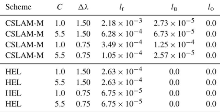
These mixing statistics include real mixing, lr, range-preserving unmixing,lu, andovershooting,lo. The more pre-cise definitions oflr,lu, andloare provided in Appendix B.
The error norm,lo, should always be zero, indicating that the scheme in question is shape preserving. However, the second norm,lu, which ideally should be zero as well, will generally not be zero, unless the scheme is semi-linear and monotone (Thuburn and McIntyre, 1997). This was one of the motivational factors for the development of HEL. The first norm,lr, should be a non-zero value, since real mixing is always present; it should, however, as described in Sect. 3, not be artificial numerical mixing but physically based mix-ing.
0.1 0.2 0.3 0.4 0.5 0.6 0.7 0.8 0.9 1.0
τ
0 20 40 60 80 100 120 140
lf
Filament preservation, 0.75◦
CSLAM-CN1.0 CSLAM-CN5.5 HEL-E-CN1.0 HEL-E-CN5.5 HEL-CN1.0 HEL-CN5.5
0.1 0.2 0.3 0.4 0.5 0.6 0.7 0.8 0.9 1.0
τ
0 20 40 60 80 100 120 140
lf
Filament preservation, 1.5◦
CSLAM-CN1.0 CSLAM-CN5.5 HEL-E-CN1.0 HEL-E-CN5.5 HEL-CN1.0 HEL-CN5.5
Fig. 8.Diagnostics for filament preservation,lf, for the two resolutions 1.5◦(left) and 0.75◦(right). The curves show the shape-preserving CSLAM-M (crosses), HEL in Eulerian grid (squares), and the HEL in Lagrangian space (circles). Each scheme is shown with a maximum Courant number of 1.0 (dotted line) and 5.5 (solid line), respectively.
Table 6.Mixing diagnosticslr,lu, andlofor CSLAM-M and HEL for two equatorial resolutions (1.5◦and 0.75◦) and two maximum Courant numbers (1 and 5.5). The columns show scheme, maximum Courant number (C), equatorial resolution in degrees (1λ), and the three error norms, respectively.
Scheme C 1λ lr lu lo
CSLAM-M 1.0 1.50 2.18×10⁻³ 2.73×10⁻⁵ 0.0 CSLAM-M 5.5 1.50 6.28×10⁻⁴ 6.73×10⁻⁵ 0.0 CSLAM-M 1.0 0.75 3.49×10⁻⁴ 1.25×10⁻⁴ 0.0 CSLAM-M 5.5 0.75 1.05×10⁻⁴ 2.57×10⁻⁵ 0.0
HEL 1.0 1.50 2.63×10⁻⁴ 0.0 0.0
HEL 5.5 1.50 2.63×10⁻⁴ 0.0 0.0
HEL 1.0 0.75 6.75×10⁻⁵ 0.0 0.0
HEL 5.5 0.75 6.75×10⁻⁵ 0.0 0.0
4.3 Deformational passive advection with divergence
Traditionall2andl∞error norms for the strongly divergent flow are presented in Table 7 for the cosine hill initial condi-tion. In this case the two maximum Courant numbers tested are 0.6 and 3.2, respectively, and it can be seen that HEL is now considerably more accurate than CSLAM-M, particu-larly for the small Courant number tested. As for the non-divergent case HEL is relatively insensitive to the Courant number.
5 Implementation and tests in a shallow water dynamical model
In this section we demonstrate a dynamical application of HEL namely as a transport scheme also for the dynamical core of an existing geophysical type model, namely a sim-ple shallow water model in Cartesian geometry (Kaas, 2008).
Despite the simple geometry applied in this model it does in-clude the fundamental processes and thereby potential prob-lems in the shallow water framework.
5.1 Model setup
The governing differential equations are du
dt =f v−g
∂(h+hs)
∂x (35)
dv
dt = −f u−g
∂(h+hs)
∂y (36)
dh
dt = −h∇ ·V+Dh+Fh (37)
dhm
dt = −hm∇ ·V+Cm+Sm+Dm, m=1, . . . , M, (38)
whereu,vare the flow speed components in thex–yplane,f
is the Coriolis parameter,gthe gravitational acceleration,h
is the geopotential thickness of the flow, andhsthe stationary surface geopotential height (“topography”).hmis a quantity
we can think of as the contribution to geopotential height from them’th tracer. The mixing ratio for them’th tracer can be evaluated from
qm=hm/ h, (39)
i.e., formally the volume density for this tracer is ρm=
ρhm/ h, whereρ is the density of the dry fluid in the
shal-low water model. It has been assumed thatPhm≪hsince,
otherwise, the expression in Eq. (39), which formally rep-resents specific density, would not approximate mixing ra-tio. The termFhrepresents a weak globally mass-conserving
Newtonian relaxation towards the initial “zonal” average pro-file ofh.Fhmimics the effect of diabatic processes. Finally
Table 7.As Table 1 but for the cosine hill problem in strongly divergent flow. Note that the maximum Courant numbersCin this case are different from those of Table 1.
CSLAM-M HEL
C λ l2 l∞ l2 l∞
0.6
3.00 3.184×10⁻¹ 4.400×10⁻¹ 5.253×10⁻² 7.607×10⁻² 1.50 9.755×10⁻² 2.048×10⁻¹ 1.580×10⁻² 2.638×10⁻² 0.75 2.346×10⁻² 7.629×10⁻² 4.711×10⁻³ 1.034×10⁻²
3.2
3.00 1.942×10⁻¹ 3.034×10⁻¹ 5.621×10⁻² 8.342×10⁻² 1.50 4.220×10⁻² 1.132×10⁻¹ 1.661×10⁻² 2.578×10⁻² 0.75 8.351×10⁻³ 3.965×10⁻² 4.848×10⁻³ 1.293×10⁻²
Althoughu,v, andhdo not depend on thehmvalues of
the tracers, the model is formally set up as “online coupled” (see, e.g., Grell and Baklanov, 2011); i.e., all equations are solved each time step.
The integration domain covers a domain defined byx∈ [xmin, xmax]andy∈ [ymin, ymax], withxmin=0 km,xmax= 20 000 km,ymin= −10 000 km, and ymax=10 000 km. The boundary conditions are periodic in both directions and with enforced symmetry around the line y=0 (“Equator”) for the variablesu,h,hs,Fh, and hm, m=1, . . . , M, and
anti-symmetry around the same line forv. Also, the Coriolis pa-rameter
f =2sin
π y ymax−ymin
is anti-symmetric aroundy=0 (is the angular velocity of the Earth rotation).
As for the inert tracer applications tested above the strat-egy followed for applying HEL in the shallow water model is to use parcel densities/geopotential thicknesses to mod-ify an existing solution in Eulerian space. As the underly-ing solution we have used a locally mass-conservunderly-ing, semi-Lagrangian transport scheme LMCSL (i.e., not the CSLAM as above) with a semi-implicit treatment of the gravity– inertial wave terms, in combination with an Arakawa C-grid staggering; see Kaas (2008) for details.
In the present implementation we have only applied the HEL technique on the mass fields (h and the hm’s) of the
model. The wind field forecast is based on the same third-order semi-Lagrangian scheme as in Kaas (2008).
As for the case of passive/inert advection the divergent expansion/contraction factors,σn+1/2, that are needed to in-clude the effects of divergence in Lagrangian space are first calculated in Eulerian space:
Eσn+1/2= Eh˜n+1
E,advhn+1, (40)
whereEh˜is the complete provisional Eulerian space forecast including semi-implicit adjustments, andE,advhis the cor-responding purely advective semi-Lagrangian forecast, i.e.,
also an Eulerian space forecast. The Eulerian space values
Eσn+1/2 are now interpolated to each parcel location (see Sect. 2.4) at time leveln+1 and subsequently multiplied on the parcel values ofLhandLhm,m=1, . . . , M. Mixing
de-pending on the flow deformation rate is then performed in Lagrangian space as described in Sect. 3
The final Eulerian space forecasts ofEh andEhm, m=
1, . . . , M are obtained via exactly the same nudging proce-dure as described above in Sect. 2.6
For the inert and passive advection tests with prescribed analytical velocities in Sect. 4 the underlying Eulerian space forecasts were all based on a first-order numerical scheme providing good numerical efficiency. Here in our dynamical model implementation we have found that it is necessary to keep third-order accurate remappings in the semi-Lagrangian scheme in order to obtain sufficiently accurate estimates of pressure gradient terms and to ensure sufficiently accurate coupling between the momentum equations (Eqs. 35 and 36), and the continuity equation (Eq. 37).
Although we have used third-order remappings it could of course still be possible to run with first-order remappings for all the tracers,m=1, . . . , M, i.e., when solving Eq. (38). In this way one can retain the same high multi-tracer efficiency as in the transport tests in Sect. 4. One may argue, though, that this violates the mass–wind consistency property, i.e., the 7th of the desired properties listed in Sect. 1. It is noted, however, that since the bulk of the model memory in HEL is kept in Lagrangian space, this is now only a theoretical prob-lem: if an inert and passive tracermis initialized ashm=h,
the Lagrangian space density of this variable will continue to be exactly equal to that ofh; i.e., at any time step nwe haveLhnm=Lhn, independent of the order of accuracy of the
underlying Eulerian-space-based forecast ofEhm.
5.1.1 Estimation of trajectories
Fig. 9.Initial height fieldh(upper left) and surface topography (upper right) for the shallow water model. The lower panel shows an example of an initial field of a single inert tracer. Only the “Northern Hemisphere” part of the fields are plotted.
obtained with a semi-Lagrangian model, as here, upstream trajectories are needed; i.e., one has to identify all departure points at timen1t for trajectories which at time(n+1)1t
end up in each Eulerian grid cell centroid. In HEL it is fur-thermore required to calculate downstream arrival points at time(n+1)1t for trajectories beginning at the irregularly spaced locations for each Lagrangian parcel at timen1t.
For the upstream trajectories we use the approach de-scribed in Kaas (2008). This is a conventional iterative proce-dure using two iterations. However, here we use third-order accurate bi-cubic Lagrange interpolations of the upstream velocities at time levelnas opposed to the first-order inter-polations in Kaas (2008). As explained in Kaas (2008), in order to ensure satisfactory behavior of the LMCSL scheme, it necessary to include the effect of accelerations in the es-timate of the trajectories. For the estimation of downstream parcel trajectories an equivalent procedure has been followed (see Appendix C for details).
5.1.2 Shallow water model results
The initial state of the shallow water model is chosen rather arbitrarily as wavy structure in the geopotential surface height field,h, shown in Fig. 9, with the velocity field (not shown) simply initialized to be in geostrophic balance with this mass field. Figure 9 also shows the bottom topography,
hs, consisting of a “sharp” isolated “mountain”, and an initial field of mixing ratio for a single tracer field, which here sim-ply is a step function in a background of zero mixing ratio.
The results obtained with HEL are compared to those ob-tained with the third-order semi-implicit LMCSL scheme (Kaas, 2008) without introduction of any shape-preserving
filters. It is noted (not shown) that one could just as well have verified HEL against a traditional implicit semi-Lagrangian (SISL) time stepping scheme, since SI-LMCSL and SISL turn out to produce almost identical forecasts. All simulations presented below have been performed with a horizontal resolution of 128×128 points cells−1. The time step was one hour, which gives a maximum Courant num-ber slightly below one. The reader is informed that LMCSL and HEL (both with and without parcel mixing) can be run stably with maximum Courant numbers up to about 3, and thereafter numerical mountain wave resonance (Rivest et al., 1994; Lindberg and Alexeev, 2000) becomes visibly destabi-lizing. No off-centering or other techniques to control moun-tain wave resonance were introduced.
Figure 10 shows the surface height field and the mixing ratio field after 48 h of simulation for the initial conditions plotted in Fig. 9. It can be seen that the geopotential height fields for each of the two forecasts are almost indistinguish-able, although the HEL result is based on densities at the locations of the irregularly spaced Lagrangian parcels. The mixing ratio fields are also similar and it can be seen that HEL via its design is shape preserving.