Adilson Jesus Teixeira*
Institute of Aeronautics and Space São José dos Campos/SP – Brazil [email protected]
*author for correspondence
Rate control system algorithm
developed in state space for models
with parameter uncertainties
Abstract: researching in weightlessness above the atmosphere needs a payload to carry the experiments. To achieve the weightlessness, the payload uses a rate control system (RCS) in order to reduce the centripetal acceleration within the payload. The rate control system normally has actuators that supply a constant force when they are turned on. The development of an algorithm control for this rate control system will be based on the minimum-time problem method in the state space to overcome the payload and actuators dynamics uncertainties of the parameters. This control algorithm uses the initial conditions of optimal trajectories to create intermediate points or to adjust existing points of a switching function. It associated with inequality constraint will form a decision function to turn on or off the actuators. This decision function, for linear time-invariant systems in state space, needs only to test the payload state variables instead of spent effort in solving differential equations and it will be tuned in real time to the payload dynamic. It will be shown, through simulations, the results obtained for some cases of parameters uncertainties that the rate control system algorithm reduced the payload centripetal acceleration below µg level and keep this way with no limit cycle.
Keywords: Rate control, Off-on control, Time optimal control, State space, Bang-bang control.
INTRODUCTION
The microgravity environment to perform experiments can be obtained in several ways. One of them uses a sounding rocket that carries a payload out of atmosphere inluence and the experiments are performed during the payload ballistic phase. After the payload separation, from the sounding rocket, the payload needs to have its angular velocity reduced in order to minimize the centripetal acceleration of the embedded equipment. To achieve centripetal acceleration to microgravity level (µg), the payload needs to have a rate control system (RCS).
The RCS for this purpose normally uses a cold gas subsystem (CGS), which is comprised of on-off actuators. This subsystem has three sets of solenoid valve thrusters, mounted in the service module skin of the payload, and each set can supply a constant torque that changes the angular velocity in one of the main payload axis.
Many publications of studies that employ on/off control, which is also named as bang-bang control, can be found. The bang-bang control has been investigated for several decades and been applied in the most different areas.
In Udrişte (2008), it is studied the controllability, observability and bang-bang properties of multi-time completely integrable autonomous linear systems described by partial differential equations (PDE). In O’Brien (2006), it is described a bang-bang control algorithm developed for a double integrator plant that can be extended to higher order plants with two integrators. This approach is studied to be used in a steering controller for an autonomous ground vehicle. Another application is the study for developing a bang-bang algorithm for a path tracking control to a differential wheeled mobile robot, where it shows that the bang-bang algorithm offers better results in accurate and time execution (Nitulescu, 2005). The switching-time computation for a bang-bang control law is developed by Lucas and Kaya (2001) to compute the switching times applied to a nonlinear system with one and after for two control inputs. Ettl and Pfänder (2009) describes the RCS used in several programs for weightlessness research in Europe and in Brazil. The aim of the RCS is to reduce the angular rates of the payload signiicantly above the atmosphere in order to minimize the centripetal accelerations to a level lower than 10 μg. This article describes the principle of a RCS. Remain publications in the references will be mentioned later in the development of the control algorithm.
Received: 04/08/11 Accepted: 06/10/11
A common problem to be solved for a RCS with a on/off control system is to obtain the instant and the duration of each control pulse to be applied to the actuators in order to reduce the payload angular velocity as close as possible to zero in minimum time, and to keep with no cycle limit amplitude. However, nonlinearities and parameters uncertainties of the system to be controlled can affect the desired performance of a designed control system.
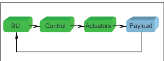
A basic RCS block diagram is shown in Fig. 1:
MATHEMATIC MODELS
A mathematic model can be a set of mathematic equations, linear or nonlinear, that approximately represents a speciic behavior of a real system.
A payload mathematical model can be represented by a LTI system in state space as shown in Eq. 1:
x'(t) = Ax(t) + Bu(t)
y(t) = Cx(t) (1)
where:
A ∈ Rn x n is the dynamic matrix; B ∈ Rn x p is the control matrix; C ∈ Rp x r is the output matrix; x(t) ∈ Rn is the state vector; u(t) ∈ Rr is the control vector; and y(t) ∈ Rp is the output vector.
To develop the equations, terms that indicate function of t
are going to be omitted.
In order to show the development of the RCS algorithm and its performance, it was used the payload and actuator mathematical models for the main X axis.
Payload mathematical model
The payload mathematical model, according to Cornelisse, Schöyer and Wakker (1979), is represented here by a linear time invariant system of a rigid body, symmetric around body X axis. For microgravity experiments, the payload is controlled only during its ballistic trajectory phase above the atmosphere when its inluence can be neglected; therefore, no external perturbation is considered. Based on these simpliications, the payload model can be represented by Eq. 2:
p'
[ ]
= 0[ ]
p+ lxIxx
¬ ®
¼
¾
½2Fa
(2)
where:
p: roll angular velocity (“roll-rate”), in [rad/s];
lx: arm of the actuator force, in [m];
Ixx: inertial momentum around body X axis, in [Kg m2]; Fa: force of each actuator, in [N], perpendicular to the body X axis. The actuator force is multiplied by two because there are two actuators for roll control, one at each opposite side of payload skin, to avoid body translation.
where:
SU: represents the sensor unit that measures the angular velocities and accelerations of the payload at its three main axes;
Control: represents the control unit that can be programmed with the control algorithm to turn on and off the actuators; and
Actuators: represents the actuators units used to change the payload angular velocity.
One method to develop a control system for on/off actuators can be found in minimum-time problem, in optimal control theory. This method permits to calculate the optimal time to turn on and off the actuators and, consequently, to get the optimal payload trajectory in the state space. Based on this, it will be developed a modiied method that uses the initial conditions for an optimal trajectory to create or adjust a switching function.
Minimum-time problem has a good performance when the parameters of a dynamic system are well known, but this performance is affected when there are parameter uncertainties. Therefore, the switching function must be created or adjusted to these uncertainties in real time.
In this paper, it will be shown the performance and how to adjust the RCS control algorithm for the following parameter uncertainties: payload mass, payload inertial momentum, actuator torque level, and/or actuator response delay. This control algorithm also has the advantage that it does not require great effort in processing.
SU Control Actuators Payload
To design the RCS it was considered that the payload mathematical model parameters have the values given by Eq. 3:
lx= 0.5 m
Ixx= 30 kg m2 (3)
Actuator mathematical model
The actuator mathematical model is represented here by an on/off second order system, with the following parameters: steady state force of 2 N, rise time (tr) of 50 ms, at 10% of steady state error, and damping ratio of 1.0; and an on/off input control ua. The hysteresis and the electromechanical delay that may affect the actuator response are not considered. Based on these simpliications, the actuator model can be represented by the LTI of Eq. 4 (Ogata, 1982):
x'a1 x'a2
¬ ® ¼ ¾ ½ ½= 0 1 -6006.25 -155 ¬ ® ¼ ¾
½ xxa1
a2 ¬ ® ¼ ¾ ½ ½+ 0 6006.25 ¬ ® ¼ ¾
½ua
Fa = 1 0¬® ¼¾ xa1
xa2
¬ ® ¼ ¾ ½ ½ (4)
where:
xa: actuator state vector;
ua: input control: value 1 (Actuator ON) and value 0 (Actuator OFF); and
Fa: actuator force, in [N].
The actuator response to unitary pulse width command of 0.3 s is shown in Fig. 2. The input signal is represented by a black dash line and the actuator force response by the blue solid line.
can be incorporated into the model. Considering model uncertainties structured, the LTI model can be represented by Eq. 5:
x ' = A +
)Ax + B + )B[u +)u] y(t) = C + )Cx + sa(5)
where:
∆A, ∆B and ∆C denotes plant parameter uncertainties, ∆u is the input parameter uncertainty,
sa is the sensor additive noise measurement.
RCS DESIGN
To explore the performance of the CGS, it is necessary to control the actuator during its steady state and its transient response. The problem is how to calculate the moment and pulse width to be applied to the actuator for these completely different behaviors.
There are many methods to design a control law for an on/off actuator. Bryson and Ho (1997) presented a design, using the minimum-time problem method in state space to get the optimal trajectory. As there are parameter uncertainties in the mathematical models, it was used this concept to develop a control algorithm that the control law could self adjust to these parameters in real time. Some generic cases of phase plane approach can be found in Ogata (1982) and of state space approach can be found in Takahashi, Rabins and Auslander (1972).
Switching function design
The irst approach of designing a rate control system in state space for a system, which has parameters uncertainties, is presented in Teixeira (2009). Here it is presented an improvement of this approach in order to get better performance and to reduce the limit cycle.
Choosing the state variable p and p’ for the state space, the optimal trajectory is that one, which takes the payload state from an initial state to a inal one, considered here the origin of state space, in minimum time. As can be seen in Fig. 2, after turning off the actuator there is a residual thrust that affects the payload state. Therefore, for the system control purpose this residual thrust need to be considered when getting optimal trajectory. Considering that the actuator is turned off during its positive or negative steady state, it can be obtained two optimal trajectories from these respectives payload mathematical model states towards the state space origin. These optimal trajectories are shown in Fig. 3.
Model parameter uncertainties
If uncertainties about the model or unmeasured inputs to the process are structured (Frisk, 1996), that is, it is known how they enter at the system dynamics; this information
0 0 0.5 1 Force [N] 1.5 2
0.05 0.1 0.15 0.2 0.25 Time [s]
0.3 0.35 0.4 0.45 0.5
These optimal trajectories could be used as a decision for the control algorithm only if the actuator was turned off from its steady state, but as it is desired to explore the CGS performance, the RCS control algorithm needs to operate also during the actuator transient response, therefore, it is necessary to build the optimal trajectories for various pulse width command during the actuator transient response.
Figure 4 shows the angular acceleration of the payload mathematical model, in time, when the actuator is turned on and off during its transient response.
as those used for the payload and actuator mathematical models. Therefore, the switching function presented in Fig. 5 will not keep the performance designed for the RCS. Thus, this algorithm must be adjusted to these unknown values.
The dynamic behavior of the real payload will be only obtained during the moment that it receives any input command, therefore, the switching function must be created or adjusted in real time. The easiest way to create it will be through linear segments connecting each point obtained for the switching function. Therefore, to begin this process the switching function is initially represented by two linear segments, one between the points in state space (-pMax, p´Max) and (0, 0) and another between points (0, 0) and (pMax, - p´Max). These segments are the initial conditions for the optimal trajectory from Fig. 5. Additional points shall be added or adjusted after each measure of the state vector error, which will be explained later.
-2 -0.08 -0.06 -0.04 -0.02 0 0.02
p’
[rad/s/s]
0.04 0.06 0.08
-1.5 -1 -0.5 0
p [rad/s]
0.5 1 1.5 x 10⁻³
2
Figure 3. Optimal trajectory that moves the payload mathematical model state vector to the state space origin.
Through several simulations, with various pulse width for the actuator operating in its transient response, and rebuilding the respective optimal trajectories, it is possible to get the initial condition, where the actuator should be turned off. By interpolating all initial conditions, it is possible to obtain one curve that will split the state space where the actuator must be turned on or off. This curve will be called switching function and it is shown in Fig. 5.
Control law design
To design the control law, it must be considered that the payload and actuator dynamic parameters are not the same
p’
[N]
0 0.01 0.02 0.03 0.04 0.05 0.06 0.07 0.08
0.05 0.1 0.15 0.2 0.25 Time [s]
0.3 0.35 0.4 0.45 0.5
Figure 4. Angular acceleration of the payload mathematical model for three different pulse width commands during the actuator transient response.
0.08
0.06
0.04
0.02
-0.02
-0.04
-0.06
-0.08 0
-2 -1.5 -1 -0.5 0 0.5 1 1.5 2
x 10-3
p’
[rad/s
2]
p [rad/s]
Figure 5. Switching function to control the payload when its actuator is commanded during its transient response.
After several simulations, it was observed that the inal conditions of the switching function for the RCS algorithm needed to be changed a little bit and had to to be added some inequality constraints (Bryson et al., 1997) to compensate the simulation step and to reduce the limit cycle amplitude, when angular velocity of the payload mathematical model is close to zero. These inequality constraints and the switching function compound a decision function that will generate the conditions to turn on or off the actuator.
where:
pMax: maximum negative angular velocity value of the switching function;
-2pMin: twice the desired increment for the negative angular velocity of the switching function;
-pMin and pMin: angular velocity precisions according to microgravity level speciied;
p’Max: maximum positive angular acceleration value of the switching function; and
-p’Min and p’Min : angular accelerations to measure the state vector error related to the state space origin.
The decision function for negative angular velocity that controls the positive actuator is compounded by four areas and two transitions described below:
• Red Area: the payload angular velocity must be reduced. The positive actuator must be turned on.
• Blue Area: close to the speciied state space area for low gravity level (green area). The control algorithm for this area will generate command pulses to the actuator to drive the payload state vectors to the state space origin.
• Green Area: corresponds to the state space area around the state space origin to get the desired low gravity level. At this area, the algorithm control must keep the actuator turned off.
• White area: corresponds to the payload state vector where the actuator must be turned off.
• Transition A: payload state vector when the control algorithm generates the command to turn off the actuator. The correspondent angular velocity of the switching function will be able to be adjusted.
• Transition B: payload state vector when the angular acceleration reaches the range from –p’Min to p’Min. The payload angular velocity measured will be used to adjust the value of the angular velocity stored at the switching function when occurs the Transition A.
Note: the best control law to generate the pulses for the blue area is under study. A good response was obtained for a pulse width equals to one step integration (1 ms) and pulse period equals to the actuator falling time (50 ms). By this way the payload state vector moves toward the origin of the state space.
The control law must use the following tests, according to each area:
1. Red Area: Actuator ON
p< Sf(p')
Up< -pMax(6)
2. Blue Area: Actuator ON/OFF (Pulse Commands)
(7)
3. Green Area: Actuator OFF
(8)
4. White Area: Actuator OFF
remain (p, p’) states while p’ > p’Min (9)
where:
Sf(p’) is the switching function in function of p’.
-pMax
Transition A
Transition B ON
ON/
OFF OFF
OFF
-2pMin -pMin
-p’Min p’Min p’Max p’
p
pMin
To adjust or create a switching function segment, according to the payload dynamic, the RCS algorithm needs to process the following steps:
• detect the Transition A;
• store the payload state vector (pA, p’A);
• detect the Transition B;
• obtain the state vector error that is the payload state vector at transition B;
• if the state vector error is outside the blue and green areas do the correction of the switching function:
If there is not a segment for (pA, p’A), then create it; else correct the stored value of the angular velocity of the switching function through the Eq. 10:
Sf (p’A) = pA – pb (10)
Regarding to the decision function for the control of the positive angular velocity, appropriate considerations shall be made in order to develop the whole algorithm control.
RCS ALGORITHM PERFORMANCE
The RCS algorithm performance was veriied through simulation to evaluate its behavior and the limit cycle amplitude of the payload angular velocity. To do so, it was used an angular velocity range from (-1.0 to +1.0) e-4rad/s as the inal payload angular velocity. These values represent a range from (-5 to +5) e-9 m/s2 that is lower than the needed one to get the microgravity condition for the parameters values of payload mathematical model given by Eq. 3. This velocity angular range was used to test the limit cycle amplitude that would be generated by the RCS algorithm. The initial values used for simulation were:
• Initial payload roll angular velocity: p0=0.005 rad/s (initial value used only for graphical purposes).
• Maximum values for the switching function, obtained from Fig. 5:
|pMax| = 1.7e-3 rad/s and |p’
Max| = 7.0e -2 rad/s2.
• Angular and acceleration steps for the switching function:
|pMin| = 1.0e-4 rad/s and |p’
Min| = 4.1e -3 rad/s2.
It was also considered the noise at sensors measures in the simulations. This noise was modeled as a color noise with Gaussian distribution, given by Eq. 11, which was added to the true sensor measure:
f
x |ȝ,ı= 1ı 2ʌ
e - x-ȝ2
2ı2
(11)
where:
μ=0 is the noisemean;
σav=2e
-5 rad/sis the noise standard deviation for angular
velocity;
σaa=2e
-5 rad/s2is the noise standard deviation for angular
acceleration.
The simulations were performed using: Simulink version 6.3, MatLab, version R14 SP3, Dormand-Prince solver and 1 ms integration step. The RCS performance is shown in the following cases.
Case I
In case I, the payload and actuators mathematical models have the nominal parameters speciied for the RCS design given by Eq. 3 and 4. Figure 7 shows a state space with the payload trajectory toward the state space origin, where: black solid line represents the payload state vector trajectory; red dashed line represents the maximum angular velocity for the switching function; solid red lines represent the switching function; blue solid lines represent the limit area for the on/off control; and green dashed lines represent the range speciied for the angular velocity and acceleration near the vector state space origin. The abscissa axis is used for angular velocity in [rad/s] and the ordinate axis is used for angular acceleration [rad/s2].
-2 -0,08 -0,06 -0,04 -0,02 0 0.02 0.04 0.06 0.08
-1 0 1
p [rad/s] x 10-3
p’
[rad/s
2]
2 3 4 5
It can be seen in Fig. 7 that the RCS algorithm turn the negative actuator on and after some time turn it off in the optimal time to drove the payload state vector close to the state space origin in minimum time.
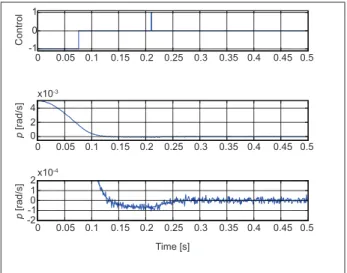
Figure 8 shows the actuator control signal and the respective payload angular velocity in time representation. First graphic represents the control signal to the actuator, where positive values correspond to the commands for positive actuator and negative values correspond to the commands for the negative one. Second graphic corresponds to the payload angular velocity and the third graphic is the magniied payload angular velocity in the speciied desired range for the design (-pMin < p, pMin).
p
[rad/s]
0 -2 -1 0 1 2x10
-4
0.05 0.1 0.15 0.2 0.25
Time [s]
0.3 0.35 0.4 0.45 0.5
p
[rad/s]
0 2 4
x10-3
0 0.05 0.1 0.15 0.2 0.25 0.3 0.35 0.4 0.45 0.5
Control
-1 0 1
0 0.05 0.1 0.15 0.2 0.25 0.3 0.35 0.4 0.45 0.5
Figure 8. Actuator control signal and payload mathematical
model angular velocity for nominal parameters. p [rad/s]
p’ [rad/s
2]
-2 -0.08 -0.06 -0.04 -0.02 0 0.02 0.04 0.06 0.08
-1 0 1 2 3 4 5
x10-3
Figure 9. Payload matethematical model state vector trajectory for case II parameters.
The payload mathematical model angular velocity was reduced to the desired range at minimum time with no limit cycle. It can be seen a small pulse width command to the positive actuator. This command was generated due to the noise at the angular velocity measure.
Case II
Case II shows the RCS algorithm performance considering the following parameters changes to the mathematical models: mass is 20% heavier, which increases the inertial momentum (Ixx = 36 kg m2); the actuator is faster, its rise time was 30% reduced (tr = 35 ms), and the actuator force was 25% reduced (Fa = 1.5 N).
Figure 9 shows the payload state vector trajectory. It can be noted that the negative actuator was initially turned off before the optimal time, related to the new payload and actuator dynamic characteristics. As the payload state vector did not reach the area speciied in the state space to
get the desired low gravity level, the RCS control algorithm created one segment for the switching function, according to the error measured during the transition B and generated another command to the negative actuator to drive the payload state vector to the origin of the state space.
Comparing Fig. 9 to Fig. 7, it can be seen that the changes at the switching function were due to the changes of the payload and actuator dynamic parameters.
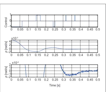
Figure 10 shows the time response of the actuator control signal and the respective payload angular velocity. First graphic shows the control signal to the negative actuator. Second graphic shows the behavior of the payload angular velocity and the third one is a magniied view of the angular velocity graphic to show that the payload angular velocity was reduced to the desired angular velocity range and it was maintained within this range with no limit cycle.
Figure 10. Actuator control signal and plant angular velocity for case II parameters.
p
[rad/s]
-2-1 0 1 2x10⁻⁴
Time [s]
0 0.05 0.1 0.15 0.2 0.25 0.3 0.35 0.4 0.45 0.5
p
[rad/s]
0 2 4
x10-3
0 0.05 0.1 0.15 0.2 0.25 0.3 0.35 0.4 0.45 0.5
Control -1
0 1
p
[rad/s]
-2 -1 0 1
2x10
-4
Time [s]
0 0.05 0.1 0.15 0.2 0.25 0.3 0.35 0.4 0.45 0.5
p
[rad/s]
-2 0 2 4
0 0.05 0.1 0.15 0.2 0.25 0.3 0.35 0.4 0.45 0.5
x10-3
0 0.05 0.1 0.15 0.2 0.25 0.3 0.35 0.4 0.45 0.5
Control -1
0 1
Figure 12. Actuator control signal and plant angular velocity for case III parameters.
CONCLUSION
It was shown that a RCS algorithm developed presents good performance, although there are uncertainties at the payload and actuators dynamic parameters.
Using the state space approach, as the time is implicit; the system control needs only to test the state vector in state space instead to solve partial differential equations. Based on minimum-time problem method for an on/off control system, adding some additional inequality constraints and the capability for the control algorithm to adjust the switching function, it is possible to converge the payload state vector to a feasible desired range, although the payload and actuators have dynamic parameter uncertainties.
Note that each point added to the switching function represents the optimal state to turn off the actuator. If this condition happens again, the state trajectory will follow the optimal trajectory.
It was shown through simulation that the RCS algorithm could self adjust to parameter uncertainties such as:
±20% of payload mass change, ±30% of actuator rise time, and ±25% of actuator force.
REFERENCES
Bryson, Jr., Arthur, E., Ho, Yu-Chi, 1997, “Applied Optimal Control – Optimization, Estimation and Control”, Hemisphere Publishing Corporation, USA.
Case III
Case III shows RCS algorithm performance considering the following parameters changes to the mathematical models: the payload mass is 20% lighter, which reduces the inertial momentum (Ixx = 24 kgm2); the actuator is slower, its rise time was increased for 30% (tr = 65 ms); and the actuator force was increased for 25% (Fa = 2.5 N).
Figure 11 shows the payload state vector trajectory. It can be noted that the negative actuator was turned off initially after its optimal time, related to the new payload and actuator dynamic characteristics. As the payload state vector did not reach the low gravity level speciied in the state space, the RCS control algorithm changed the maximum positive angular velocity of the switching function from (1.7 to 3.1) e-3rad/s, according to the error measured during the transition B. After that, the RCS control algorithm generated commands and created segments to the switching function.
p’
[rad/s
2]
p [rad/s] -2
-0.1 -0.08 -0.06 -0.04 -0.02 0 0.02 0.04 0.06 0.08
-1 0 1 2 3 4 5
x10-3
Figure 11. Payload matethematical model state vector trajectory for case III parameters.
Cornelisse, J. W., Schöyer, H. F. R., Wakker, K. F., 1979, “Rocket Propulsion and Spacelight Dynamics”, Pitman Publishing Limited, London, England.
Ettl, J., Pfänder, J., 2009, “Rate Control System for Sounding Rockets”, 19th ESA Symposium on European Rocket and Balloon Programmesand and Related Research, Bad Reichenhall, Germany, (ESA SP-671).
Frisk, E., 1996, “Model-Based Fault Diagnosis Applied To A Si-Engine”, Linköping University, Linköping, Sweden.
Lucas, S. K., Kaya, C. Y., 2001, “Switching-Time Computation for Bang-Bang Control Laws”, Proceedings of the American Control Conference, Arlington, VA, USA.
Nitulescu, M., 2005, “Controlling a Mobile Robot Along Planned Trajectories”, Control Engineering and Applied Informatics, Vol. 7, N. 2, p. 18-24.
O’Brien Jr., R.T., 2006, “Bang-Bang Control for Type-2 Systems”, Proceedings of the 38th Southeastern Symposium on System Theory, Tennessee Technological University, Cookeville, TN, USA.
Ogata, K., 1982, “Modern Control Engineering”, Editora Prentice/Hall do Brasil Ltda, Rio de Janeiro, RJ, Brazil.
Takahashi, Y., Rabins, M. J., Auslander, D. M., 1972, “Control and Dynamic Systems”, Addison-Wesley Publishing Company, Massachusetts, USA.
Teixeira, A. J., 2009, “Rate Control System For Plant Parameter Uncertainties”, Proceedings of the 19th ESA Symposium on European Rocket and Balloon Programmes and Related Research, SP-671 pg. 255-260, Bad Reichenhall, Germany.