Shirley C. C. Nascimento
Emanuel N. Macêdo
Member, ABCMJoão N. N. Quaresma
Sênior Member, ABCM[email protected] Chemical and Food Engineering Department Universidade Federal do Pará – UFPA Campus Universitário do Guamá Rua Augusto Corrêa, 01 66075-110 Belém, PA, Brazil
Generalized Integral Transform
Solution for Hydrodynamically
Developing Non-Newtonian Flows in
Circular Tubes
The Generalized Integral Transform Technique (GITT) is applied to the solution of the momentum equations in a hydrodynamically developing laminar flow of a non-Newtonian power-law fluid inside a circular duct. A primitive variables formulation is adopted in order to avoid the singularity of the auxiliary eigenvalue problem in terms of Bessel functions at the centerline of the duct when the GITT approach is applied. Results for the velocity field and friction factor-Reynolds number product are computed for different power-law indices, which are tabulated and graphically presented as functions of the dimensionless coordinates. Critical comparisons with previous results in the literature are also performed, in order to validate the numerical codes developed in the present work and to demonstrate the consistency of the final results.
Keywords: Generalized integral transform technique, non-Newtonian fluids, power-law
model, hydrodynamically developing laminar flow, primitive variables formulation
Introduction
The analysis of hydrodynamically developing laminar flows inside ducts of cylindrical geometry has been a subject of great interest as demonstrated by the currently literature, mainly to the interest in flows within concentric circular ducts. Therefore, a correct prediction related to the heat transfer between the channel wall and the fluid studied is extremely important in equipment design and thermal devices in general. Heat transfer to purely viscous non-Newtonian fluids is frequently encountered in various industrial processes (e.g., chemical, petrochemical and food processing). These fluids are commonly processed under laminar flow conditions because of their high apparent viscosities and also the small hydraulic diameters employed in compact heat exchangers. An important feature of most purely viscous non-Newtonian fluids is that some of their rheological and thermophysical properties are very sensitive to temperature. This variation can have a large effect on the development of the velocity and temperature profiles, consequently on the pressure drop and heat transfer rates.1
A brief literature survey indicates that Lin and Shah (1978) have studied the heat transfer problem of power-law fluids with yield stress, flowing in the entrance region of a circular duct and of parallel plates; they used a forward marching procedure to solve the related momentum and energy equations. Cuccurullo and Berardi (1998) investigated the simultaneously developing of velocity and temperature profiles in the entrance pipe flow. The flow was assumed to be steady state for a non-Newtonian fluid in incompressible laminar pipe flow. The fluid behavior was assumed to follow the Ostwald-de Waele power-law model. The developing velocity and temperature profiles were solved by the integral method. Results were presented and discussed in terms of axial and radial velocity profiles, Fanning friction factors and Nusselt numbers for different fluid properties and thermal boundary conditions.
In this context, the present study applies the Generalized Integral Transform Technique (GITT) in the solution of the momentum equations for a non-Newtonian power-law fluid flowing in the entrance region of circular tubes, and for this purpose, the
Paper accepted September, 2005. Technical Editor: Atila P. Silva Freire.
boundary-layer formulation in terms of primitive variables is adopted in order to avoid singularities in the auxiliary eigenvalue problem expressed as Bessel functions at the centerline of the duct. The GITT approach is an extension of the Classical Integral Transform Technique, which is based on eigenfunction expansions yielding to solutions where the most features are the automatic and straightforward global error control and an only mild cost increase in overall computational effort for multidimensional situations. The most recent contributions are aimed at finding accurate solution of non-linear heat and fluid flow problems, which include problems with variable properties, moving boundaries, irregular geometries, non-linear source terms, non-linear boundary conditions, Navier-Stokes equations and boundary layer equations (Machado and Cotta, 1991). In recent works, Quaresma (1997), Magno (1998), Nascimento (2000) and Chaves (2001) carried out important studies related to the GITT application to different kinds of problems. A detailed compilation dealing with the advances of this technique on diffusion-convection problems can be found in Cotta (1993, 1998) and Cotta and Mikhailov (1997). Numerical results for the velocity field and local Fanning friction factor are obtained considering the effect of the power-law index, and the results for velocity profile are compared with those reported in literature. The convergence behavior is also illustrated showing the consistency of the final results.
Nomenclature
Ai(R) = coefficient defined in Equation (19a) Bfdi = coefficient defined in Equation (19b) Ci = coefficient defined in Equation (19c) Dijk =coefficient defined in Equation (22a) Eijk = coefficient defined in Equation (22b) f = Fanning friction factor
i
f = coefficient defined in Equation (21) Ffdik = coefficient defined in Equation (22c) Gik = coefficient defined in Equation (22d) Hi = coefficient defined in Equation (22e)
J0, J1 =Bessel functions of the first kind of orders zero and one, respectively
K = consistency index of the fluid n = power-law index
p, P = pressure field, dimensional and dimensionless, respectively
rw = tube radius
r, R = radial coordinate, dimensional and dimensionless, respectively
Re = apparent Reynolds number
i
U (Z) = transformed potential for the velocity field UF(R,Z) = filtered potential for the velocity field Ufd(R) = fully developed longitudinal velocity
u, U = longitudinal velocity component, dimensional and dimensionless, respectively
u0 = inlet velocity
Uc = longitudinal velocity component at the centerline of the circular tube
v, V = radial velocity component, dimensional and dimensionless, respectively
X+ = dimensionless longitudinal coordinate defined in Equation (26)
z, Z = longitudinal coordinate, dimensional and dimensionless, respectively
Greek Letters δij = Kronecker delta
η = coefficient defined in Equation (3)
µi = eigenvalues of problem (14)
ρ = fluid density
ψi(R) = eigenfunctions of problem (14) )
R ( ~
i
ψ = normalized eigenfunctions
Subscripts and Superscripts
i, j, k = order from eigenvalue problem fd = referred to fully developed situation F = referred to filtered potential _ = integral transformed quantities ~ = referred to normalized eigenfunction
Analysis
Within the range of validity of the boundary layer hypothesis, the continuity and momentum equations in primitive-variables formulation for this problem are written in dimensionless form as:
( )
RV 0 R R 1 Z U = ∂ ∂ + ∂ ∂; 0<R<1; Z>0 (1)
∂ ∂ η ∂ ∂ + ∂ ∂ − = ∂ ∂ + ∂ ∂ R U R R R 1 Re 1 Z P R U V Z U
U ; 0<R<1; Z>0 (2)
where 2 1 n 2 R U − ∂ ∂ = η (3)
with the following inlet and boundary conditions:
0
Z= : U(R,Z)=1; V(R,Z)=0; (4a,b)
R=0: 0 R ) Z , R ( U = ∂ ∂
; V(R,Z)=0; (4c,d)
1
R= : U(R,Z)=0; V(R,Z)=0; (4e,f)
The dimensionless groups employed in the above equations are:
w
r r R= ;
0
u u U= ;
0
u v V= ;
w
r z Z= ;
2 0 u p P ρ = ; K r u Re n w n 2 0− ρ = (5a,f)
To improve the computational performance in the solution of the velocity field, with respect to the direct procedure (Cotta and Carvalho, 1991), the fully developed flow situation is separated from the complete potential, in the form:
) Z , R ( U ) R ( U ) Z , R (
U = fd + F (6)
− + + = + n 1 n
fd 1 R
1 n 1 n 3 ) R ( U (7)
This is a commonly used strategy in the integral transform approach (Cotta and Serfaty, 1991; Cotta, 1993) that is equivalent to the separation of the steady state solution in a transient problem, which acts by filtering the equation source terms responsible for the slower convergence rates in non-homogeneous problems. Then, after the substitution of the splitting-up scheme, Eq. (6), the problem formulation is rewritten as:
( )
RV 0 R R 1 ZUF =
∂ ∂ + ∂ ∂ (8)
(
)
+ ∂ ∂ η ∂ ∂ + ∂ ∂ − = = + − ∂ ∂ + ∂ ∂ + dR dU R U R R R 1 Re 1 Z P R n 1 n 3 R U V Z U U U fd F n 1 F F fd F (9) where 2 1 n 2 n 1 F R n 1 n 3 R U − + − ∂ ∂ = η (10)and the inlet and boundary conditions become:
0
Z= : UF(R,Z)=1−Ufd(R); V(R,Z)=0 (11a,b)
0
R= : 0
R ) Z , R (
UF =
∂ ∂
; V(R,Z)=0 (11c,d)
R=1: UF(R,Z)=0; V(R,Z)=0 (11e,f)
The next step in the solution of Eqs. (8) to (10) is the elimination of the transversal velocity component, V(R,Z), and the pressure gradient, (-∂P/∂Z). First, the continuity equation (8) is integrated, to yield:
ξ ∂ ∂ ξ
=
∫
dZ U R 1 ) Z , R ( V 1 R F (12)
(
)
1 R F fd 1 0 F F fd R U dR dU Re 2 dR Z U U U R 4 Z P = ∂ ∂ + η − ∂ ∂ + = ∂ ∂−
∫
(13)Equations (12) and (13) relate the transversal velocity and pressure gradient to the longitudinal velocity field, as required for completion of the integral transformation process. Following the formalism in the generalized integral transform technique, to construct the eigenfunction expansions, an auxiliary eigenvalue problem is selected as:
0 ) R ( R dR ) R ( d R dR d i 2 i
i +µ ψ =
ψ
; in 0<R<1 (14a)
0 dR ) R ( d 0 R i = ψ =
; ψi(R)R=1=0 (14b,c)
The eigenfunctions and the transcendental expression to calculate the eigenvalues are given, respectively, by:
) R ( J ) R
( 0 i
i = µ
ψ ; J0(µi)=0 (14d,e)
The eigenfunctions of this eigenvalue problem enjoy the following orthogonality property:
= ≠ = δ = ψ ψ
∫
j i , 1 j i , 0 dR ) R ( ~ ) R ( ~ R ij 10 i j (14f)
where ψ~i(R)=ψi(R)/ Ni is the normalized eigenfunction and the normalization integral is defined as:
( )
( )
∫
ψ = µ= 1 0 i 2 1 2 i i J 2 1 dR R R N (14g)
The problem given by Eqs. (14) allows the definition of the following integral-transform pair:
∫
ψ = 10 i F
i(Z) R~ (R)U (R,Z)dR
U , transform (15)
∑
∞ = ψ = 1 i i iF(R,Z) ~ (R)U(Z)
U , inversion (16)
In terms of the transformed potentials defined by Eq. (15), the transversal velocity component and pressure gradient are rewritten as:
∑
∞ = = 1 i i i dZ ) Z ( U d R ) R ( A ) Z , R ( V (17) dZ U d C n 1 n 3 B 2 dZ U d U 4 Z P i 1 i i fdi 1 i i j 1 j ij∑
∑ ∑
∞ = ∞ = ∞ = + − + δ = ∂ ∂ − + − ψ η −∑
∞ = n 1 n 3 U ) 1 ( ' ~ ) z , 1 ( Re 2 1 i i i (18) where[
J( ) RJ( R)]
N 1 d ) R ( ~ ) R (A 1 i 1 i
2 / 1 i i 1 R i
i µ − µ
µ = ξ ψ ξ =
∫
; dR ) R ( ~ ) R ( U RB fd i
1 0
fdi =
∫
ψ (19a,b)dR ) R ( A R C 1 0 i n 1
i=
∫
;2 1 n 2 1 i i ' i n 1 n 3 ) Z ( U ) 1 ( ~ ) Z , 1 ( − ∞ = + − ψ =
η
∑
(19c,d)Equation (9) is now integral transformed through the operator
∫
1 ψ0 i(R)dR
~
R , to yield the transformed ordinary differential
equations:
[
]
j fdik ik1 j jk i ijk ijk 1 k G n 1 n 3 F U ) 0 ( A 4 E D + − + δ − +
∑
∑
∞ = ∞ = i k k fdk i H dZ U d C n 1 n 3 B ) 0 ( A 2 = + − − (20)The inlet condition, Eq. (11a), is similarly integral transformed to provide:
[
1 U (R)]
dR ) R ( ~ R f ) 0 (Ui = i =
∫
01 ψi − fd (21)where the various coefficients in Eq. (20) are given by:
∫
ψ ψ ψ= 1
0 i j k
ijk R~ (R)~ (R)~ (R)dR
D ;
∫
ψ ψ = 10 k
' j i
ijk ~ (R)~ (R)A (R)dR
E (22a,b)
∫
ψ ψ= 1
0 fd i k
fdik RU (R)~ (R)~ (R)dR
F ;
∫
ψ= 1
0 i k
n 1
ik R ~ (R)A (R)dR
G (22c,d)
( )
A(0)n 1 n 3 U 1 ~ ) Z , 1 ( Re 2 H i 1 k k ' k i + − ψ η − =
∑
∞ =∫
∑
+ − ψ η ψ − ∞ = 1 0 n 1 k 1 k ' k 'i R dR
n 1 n 3 U ) R ( ~ ) Z , R ( ) R ( ~ R Re 1 (22e)
The inversion formula, Eq. (15), and Eq. (6) are recalled to construct the original potential for the longitudinal velocity component, in the form:
∑
=ψ + = NC 1 i i ifd(R) ~ (R)U (Z)
U ) Z , R ( U (23)
where NC is the truncation order for the velocity eigenfunction expansion.
n 1 2 2
R 1
2 U U
f
Re R R
−
=
− ∂ ∂
= ∂ ∂
;
+ −
ψ = ∂
∂
∑
∞=
= n
1 n 3 ) Z ( U ) 1 ( ~ R
U
1 i
i ' i 1 R
(24,25)
Results and Discussion
Numerical results for the velocity profiles and Fanning friction factors were produced for different values of power-law indices, namely n = 0.5; 0.75; 1.0; 1.25 and 1.5, at the entrance region of a circular tube. The computational code was developed in FORTRAN 90/95 programming language and implemented on a PENTIUM-IV 1.3 GHz computer.
First, the numerical code was validated for the case n = 1.0 (Newtonian situation) against those results presented by Hornbeck (1964) and Liu (1974), which employed the Finite Difference Method for the solution of the same problem. The routine DIVPAG from the IMSL Library (1991) was used to numerically handle the truncated version of the system of ordinary differential equation (20), with a relative error target of 10-8 prescribed by the user, for the transformed potentials. These results were produced for Re = 2000, but it should be noted that the dimensionless axial coordinate X+ makes the results independent of the apparent Reynolds number. The definition of X+ is written as:
Re Z
X+= (26)
Tables 1 to 3 show the convergence behavior of the longitudinal velocity component at the centerline of the circular tube for power law indices n = 0.5; 1.0 and 1.25, a convergence with at least three significant digits is verified. Also, for n = 1.0, the comparison with the results presented by Hornbeck (1964) and Liu (1974) demonstrates a good agreement, which provides a direct validation of the numerical code here developed. This same analysis is also shown in Fig. 1, where it is observed a monotonic convergence for the longitudinal velocity component at the centerline of the circular tube, Uc.
Table 1. Convergence behavior of the longitudinal velocity component at the centerline of the circular tube for power-law index n = 0.5.
X+ NC = 20 NC = 40 NC = 60 NC = 80
0.0002116 1.017 1.021 1.024 1.025 0.0005000 1.034 1.044 1.049 1.050 0.001058 1.066 1.078 1.083 1.084 0.001250 1.075 1.088 1.093 1.094 0.005000 1.200 1.215 1.220 1.220 0.005288 1.207 1.222 1.227 1.227 0.01204 1.329 1.345 1.351 1.351 0.01250 1.335 1.352 1.357 1.357 0.04924 1.544 1.569 1.578 1.579 0.05000 1.546 1.571 1.580 1.581 0.06250 1.566 1.592 1.602 1.603 0.06281 1.566 1.593 1.603 1.604 0.07634 1.579 1.606 1.616 1.618 0.08993 1.587 1.614 1.624 1.626
1.0 1.592 1.666 1.666 1.666
5.0 1.667 1.667 1.667 1.667
Table 2. Convergence behavior of the longitudinal velocity component at the centerline of the circular tube for power-law index n = 1.0.
X+ NC = 20
NC = 40
NC = 60
NC = 80
Hornbeck (1964)
Liu (1974)
0.0002116 1.015 1.033 1.067 1.113 - 1.100 0.0005000 1.096 1.111 1.127 1.145 1.150 -
0.001058 1.169 1.183 1.192 1.200 - 1.210 0.001250 1.187 1.201 1.209 1.215 1.227 - 0.005000 1.393 1.408 1.414 1.415 1.433 - 0.005288 1.405 1.420 1.429 1.427 - 1.439
0.01204 1.607 1.625 1.631 1.631 - 1.644 0.01250 1.618 1.636 1.642 1.642 1.660 - 0.04924 1.906 1.933 1.945 1.946 - 1.971 0.05000 1.907 1.935 1.946 1.947 1.970 - 0.06250 1.923 1.949 1.960 1.961 1.986 - 0.06281 1.923 1.949 1.960 1.961 - 1.989 0.07634 1.933 1.957 1.968 1.969 - 1.996 0.08993 1.941 1.962 1.972 1.972 - 1.999 1.0 2.000 2.000 2.000 2.000 - - 5.0 2.000 2.000 2.000 2.000 - -
Table 3. Convergence behavior of the longitudinal velocity component at the centerline of the circular tube for power-law index n = 1.25.
X+ NC = 10 NC = 20 NC = 30
0.0002116 0.9983 1.025 1.038 0.0005000 1.094 1.129 1.137 0.001058 1.185 1.219 1.227 0.001250 1.201 1.241 1.249 0.005000 1.456 1.487 1.496 0.005288 1.469 1.499 1.509
0.01204 1.704 1.739 1.751
0.01250 1.717 1.752 1.764
0.04924 1.999 2.036 2.052
0.05000 1.201 2.037 2.053
0.06250 2.023 2.050 2.064
0.06281 2.021 2.050 2.064
0.07634 2.039 2.061 2.072
0.08993 2.054 2.069 2.078
1.0 2.111 2.111 2.111
0 0.02 0.04 0.06 0.08 0.1
X+
1 1.2 1.4 1.6 1.8 2
Uc
Liu (1974) Hornbeck (1964) NC = 80 NC = 60 NC = 40 NC = 20 n = 1.0
Figure 1. Convergence behavior of the Uc velocity component for power-law index n = 1.0.
Figures 2 and 3 bring a convergence behavior of the Uc velocity component for the cases of power-law indices n = 0.5 and 1.25, and the same observations are verified as for the case of n = 1.0, i.e., a monotonic convergence for this velocity component.
0 0.02 0.04 0.06 0.08
X+
1 1.2 1.4 1.6
Uc
NC = 80 NC = 60 NC = 40 NC = 20 n = 0.5
Figure 2. Convergence behavior of the Uc velocity component for power-law index n = 0.5.
0 0.02 0.04 0.06 0.08
X+
0.8 1.2 1.6 2 2.4
Uc
NC = 30 NC = 25 NC = 20 NC = 15 NC = 10 n = 1.25
Figure 3. Convergence behavior of the Uc velocity component for power-law index n = 1.25.
Figure 4 illustrates the development of the longitudinal velocity profiles for different power-law indices, namely, n = 0.5; 0.75; 1.0; 1.25 and 1.5, as function of the transversal coordinate R, at specific axial positions X+. From this figure it can be noticed that when the power-law index increases there is an increase in the value of the centerline velocity. In regions near the tube wall, it is verified that the velocity gradient diminishes as n increases. This is due to an increase of the apparent fluid viscosity, and consequently an increase of the wall stress. For practical engineering considerations, this effect leads to an undesirable increase of the pumping power to promote the flow of this type of fluids inside circular tubes.
0 0.4 0.8 1.2 -1
-0.6 -0.2 0.2 0.6 1
R
0 0.4 0.8 1.2 0 0.4 0.8 1.2 0 0.4 0.8 1.2 1.6 0 0.4 0.8 1.2 1.6 2 n = 0.5
n = 0.75 n = 1.0 n = 1.25 n = 1.5
X+ = 0.8467x10⁻³ X+ = 0.125x10⁻² X+ = 0.375x10⁻² X+ = 0.75x10⁻² X+ = 0.225x10⁻¹
U(X+, R)
Figure 4. Development of the longitudinal velocity component along the entrance region of the circular tube for different power-law indices.
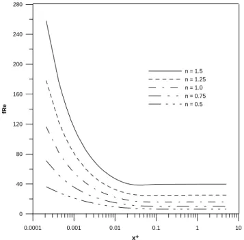
due to higher velocity gradients experimented by these fluids in this region.
0.0001 0.001 0.01 0.1 1 10
X+
0 40 80 120 160 200 240 280
fR
e
n = 1.5 n = 1.25 n = 1.0 n = 0.75 n = 0.5
Figure 5. Development of the product Fanning friction factor-apparent Reynolds number in the entrance region for different power-law indices.
Finally, Table 4 shows a comparison of the present results for the product fRe in the fully developed region against those of Quaresma and Macêdo (1998). It is verified an excellent agreement between the two sets of results, once again validating the numerical codes developed here.
Table 4. Comparison of the product fRe in the fully developed region for different power-law indices.
fRe n
Present work Quaresma and Macêdo (1998)
0.5 6.3246 6.32455
0.75 10.102 10.1023
1.0 16.000 16.0000
1.25 25.238 -
1.50 39.718 39.7175
Conclusions
Numerical results for the velocity field and product Fanning friction factor-apparent Reynolds number were produced by using the GITT approach in the solution of the momentum equations for the flow of non-Newtonian power-law fluids in circular tubes.
Results for velocity profiles indicate that an increase of the power-law index promotes an increase of the centerline velocity in order to obey the mass conservation principle, this way demonstrating the strong influence of the viscous effects on the characteristics of the fluid flow. It was also observed that the product fRe is higher for the cases of dilatant fluids (n > 1) than for those of pseudoplastic ones (n < 1) due to an increase of the apparent fluid viscosity in regions near to the tube wall.
References
Chaves, C.L., 2001, “Integral Transformation of the Momentum and Energy Equations in the Flow of Non-Newtonian Fluids in Irregular Ducts”, M.Sc. Thesis (in Portuguese), Chemical Engineering Department, Universidade Federal do Pará, Belém, Brazil.
Cotta, R.M. and Serfaty, R., 1991, “Integral Transform Algorithm for Parabolic Diffusion Problems with Nonlinear Boundary Layer and Equation Source Terms”, Proceedings of the 7th Int. Conf. Num. Meth. for Thermal Problems, Stanford, Vol. II, pp. 916-926.
Cotta, R.M. and Carvalho, T.M.B., 1991, “Hybrid Analysis of Boundary Layer Equations for Internal Flow Problems”, Proceedings of the 7th Int. Conf. Num. Meth. in Laminar and Turbulent Flow, Stanford, Vol. I, pp. 106-115.
Cotta, R.M., 1993, “Integral Transforms in Computational Heat and Fluid Flow”, CRC Press, Boca Raton, USA.
Cotta, R.M. and Mikhailov, M.D., 1997, “Heat Conduction: - Lumped Analysis, Integral Transforms, Symbolic Computation”, John Wiley, New York, USA.
Cotta, R.M., 1998, “The Integral Transforms Method in Thermal and Fluids Science and Engineering”, Begell House, New York, USA.
Cuccurullo, G and Berardi, P.G., 1998, “Developing of Velocity and Temperature in Entrance Pipe Flow for Power Law Fluids”, Proceedings of the11th International Heat Transfer Conference, Vol. 3, pp. 15-20.
Hornbeck, R.W., 1964, “Laminar Flow in the Entrance Region of a Pipe”, Applied Scientific Research, Section A, Vol. 13, pp. 224-232.
IMSL Library, 1991, MATH/LIB, Houston, TX.
Lin, T. and Shah, V.L., 1978, “Numerical Solution of Heat Transfer to Yield Power Law Fluids Flowing in the Entrance Region”, Proceedings of the 6th International Heat Transfer Conference, Vol. 5, pp. 317-322.
Liu, J., 1974, “Flow of a Bingham Fluid in the Entrance Region of an Annular Tube”, M. S. Thesis, University of Wisconsin – Milwaukee, USA.
Machado, H.A. and Cotta, R.M., 1995, “Integral Transform Method for Boundary Layer Equations in Simultaneous Heat and Fluid Flow Problems”, International Journal of Numerical Methods for Heat and Fluid Flow, Vol. 5, pp. 225-237.
Magno, R.N.O., 1998, “Solutions for the Boundary Layer Equations for a Non-Newtonian Fluid via Generalized Integral Transform Technique”, M.Sc. Thesis (in Portuguese), Chemical Engineering Department, Universidade Federal do Pará, Belém, Brazil.
Nascimento, U.C.S., 2000, “Study of the Thermal Entry Region in the Laminar Flow of Bingham Plastics in Concentric Annular Ducts”, M.Sc. Thesis (in Portuguese), Chemical Engineering Department, Universidade Federal do Pará, Belém, Brazil.
Quaresma, J.N.N., 1997, “Integral Transformation of the Navier-Stokes Equations in Three-Dimensional Laminar Flows”, D.Sc. Thesis (in Portuguese), Mechanical Engineering Department, Universidade Federal do Rio de Janeiro, Rio de Janeiro, Brazil.