Attribute Match Discovery in Information
Integration: Exploiting Multiple Facets of
Metadata
David W. Embley, David Jackman and Li Xu*
Department of Computer Science - Brigham Young University Provo, Utah 84602, U.S.A.
Phone: Voice: (801) 422-3027 Fax: (801) 422-0169 [email protected], [email protected], [email protected]
Abstract
Automating semantic matching of attributes for the purpose of information integration is challenging, and the dynamics of the Web further exacerbate this problem. Believing that many facets of metadata can contribute to a resolution, we present a framework for multifaceted exploitation of metadata in which we gather information about potential matches from various facets of metadata and combine this information to generate and place confidence values on potential attribute matches. To make the framework apply in the highly dynamic Web environment, we base our process on machine learning when sufficient applicable data is available and base it otherwise on empirically observed rules. Experiments we have conducted are encouraging, showing that when the combination of facets converges as expected, the results are highly reliable.
Keywords: semantic attribute matching, information integration, exploitation of metadata.
1 Introduction
In this paper, we focus on the long-standing and challenging problem of attribute matching [1] for the purpose of information integration. To address this problem, researchers have used a variety of techniques including the use of data values [2, 3], data-dictionary information [3], structural properties [4], ontologies [5], synonyms and other terminological relationships found in dictionaries and thesauri [6, 7, 8], and various combinations of these techniques [9, 10, 11]. These are the kinds of facets of
metadata we wish to exploit, all of which may contribute to the resolution of attribute-matching issues.
As in [12], we assume that we wish to integrate data from multiple source schemes into a target scheme, and we assume that all schemes are described using the same conceptual model [13]. Source schemes may or may not have associated populated data instance and additional metadata beyond a basic database scheme. Typical sources we consider include Web repositories, which we reverse engineer into source schemes by the data-extraction processes we have defined for semistructured and unstructured Web pages [14], by the database reverse-engineering process we have defined, which works for Web tables and relational databases [15], and by the Web form data-extraction process we are developing [16]. Moreover, using standard representational transformations among conceptual-model schemes, we can transform the conceptual-model instance of any particular wrapper into a conceptual-model instance required by our technology, and thus we can make use of any developed wrapper technology (e.g. [17, 18, 19] and many more — see the bibliography in [14]). In addition to these assumptions for sources, we assume that target schemes are augmented with a variety of both application-independent and application-speficic-ontological information. For this paper the augmentations we discuss are WordNet [20, 21], which is application independent, sample data, which is application specific, and regular-expression recognizers, which are partly application specific and partly application independent.
Our contribution in this paper is the following framework, which we propose as a way to discover which attributes in a source scheme S directly match with which attributes in a target scheme T.1
1. For each individual, independent facet,2 find potential attribute matches between the m attributes in S and the n attributes in T. Provide confidence measures between 0 (lowest confidence) and 1 (highest confidence) for each potential match. Section 2 explains how we generate matching rules over independent facets.
2. Using the confidence measures from (1), combine the measures for each potential match into a unified measure of match confidence. The result is an m x n matrix M of confidence measures. The last subsection of Section 2 explains how we combine confidence measures.
3. Using the matrix of combined confidence measure from (2), apply a structural test to further refine the confidence-measure matrix M. Section 3 explains how we apply this test.
4. Iterate over M obtained from (3) using a best-first match constrained by an injective assignment algorithm until all matches whose confidence measures exceed a predetermined threshold are settled. Section 4 explains how we settle attribute matches.
Although we have some idea about what metadata is most useful and in what combination and under what circumstances we should use this metadata, we do not know with certainty. Thus, rather than try to encode algorithms over the metadata ourselves, we use machine learning, where possible, to develop the algorithms. This approach also has the advantage of being flexible in the presence of changing dynamics, which are so common on the Web.
We illustrate our framework using car advertisements, which are plentiful on the Web, appearing in a variety of unstructured and structured forms. In Section 5 we report on the results obtained from this application.
Sometimes we are not able to make use of all facets of metadata. Targets may not have sample data, for example, and sometimes they may not have data descriptions. Sometimes source schemes are known, but data has either not yet been provided or is not available.
In these cases, even though we cannot make use of all facets of metadata, we can still run our multifaceted attribute-matching process by considering the facets we do have. We discuss the case of having only two facets, namely
terminological relationships and structural properties, in Section 6. We also give results for three additional applications: music CDs, genealogy, and real estate.
In Section 7 we summarize, draw conclusions, and give guidance for future work.
2 Independent Facet Matching
We have investigated three independent facets: (1) terminological relationships (e.g. synonyms, word senses, and hypernym groupings), (2) data-value characteristics (e.g. average values, variances, string lengths), and (3) target-specific, regular-expression matches (i.e. whether expected strings appear in the data). For each independent facet we obtain a vector of measures for the features of interest and then apply machine learning over this feature vector to generate a decision rule and a measure of confidence for each generated decision. We use C4.5 [22] as our decision-rule and confidence-measure generator.
In the subsections below, we explain the details about how we generate confidence values for source-target attribute pairs for the independent facets we have investigated. Then, in a subsequent subsection we explain how we combine the confidence values obtained from the independent facets into a single combined confidence-value matrix for each pair of source-target attributes.
2.1 Terminological Relationships
One facet of metadata that provides a clue about which attributes to match is the meaning of the attribute names. To match attribute names, we need a dictionary or thesaurus. WordNet [20, 21] is a readily available lexical reference system that organizes English nouns, verbs, adjectives, and adverbs into synonym sets, each representing one underlying lexical concept. Other researchers have also suggested using WordNet to match attributes (e.g. [7, 23]), but have given few, if any, details.
f3 <= 0: NO (222.0/26.0) f3 > 0
I f2 <= 2: YES (181.0/3.0) I f2 > 2
I I f4 <= 11
I I I f2 <= 5: YES (15.0/5.0) I I I f2 > 5: NO (14.0/6.0) I I f4 > 11: NO (17.0/2.0)
Figure 1: Generated WordNet Rule
1 In future work we intend to expand this framework to indirect
matches in which target object and relationship sets match with virtual source object and relationship sets formed by queries over source model instances as set forth in [12], but we focus here only on direct attribute matches.
2 All facets except structural facets are independent. Since structural
Initially we investigated the possibility of using 27 available features of WordNet in an attempt to match an attribute A of a source scheme with an attribute B of a target scheme. The C4.5-generated decision tree, however, was not intuitive.3 We therefore introduced some bias by selecting only those features we believed would contribute to a human’s decision to declare a potential attribute match, namely (f0) same word (1 if A = B and 0 otherwise), (f1) synonym (1 if “yes” and 0 if “no”), (f2) sum of the distances of A and B to a common hypernym (“is kind of”) root (if A and B have no common hypernym root, the distance is defined as a maximum number in the algorithm), (f3) the number of different common hypernym roots of A and B, and (f4) the sum of the number of senses of A and B. For our training data we used 222 positive and 227 negative A-B pairs selected from attribute names found in database schemes, which were readily available to us, along with synonym names found in dictionaries. Figure 1 shows the resulting decision tree. Surprisingly, neither f0 (same word) nor f1 (synonym) became part of the decision rule. Feature f3 dominates - when WordNet cannot find a common hypernym root, the words are not related. After f3, f2 makes the most difference - if two words are closely related to the same hypernym root, they are a good potential match. (Note that f2 covers f0 and f1 because both identical words and direct synonyms have zero distance to a common root; this helps mitigate the surprise about f0 and f1.) Lastly, if the number of senses is too high (f4 > 11), a pair of words tends to match almost randomly; thus the C4.5-generated rule rejects these pairs and accepts fewer senses only if pairs are reasonably close (f2 <= 5) to a common root. The parenthetical numbers (x I y) following “YES” and “NO” for
a decision-tree leaf L give the total number of training instances x classified for L and the number of incorrect training instances y classified for L.
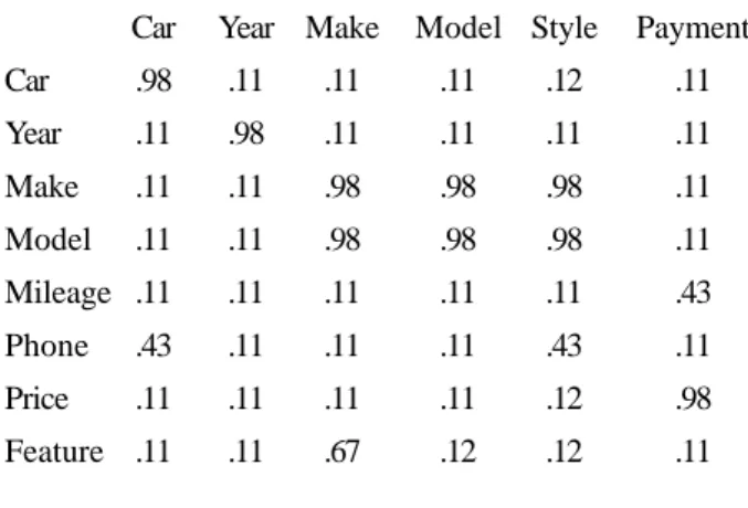
Car Year Make Model Style Payment
Car .98 .11 .11 .11 .12 .11
Year .11 .98 .11 .11 .11 .11
Make .11 .11 .98 .98 .98 .11
Model .11 .11 .98 .98 .98 .11
Mileage .11 .11 .11 .11 .11 .43
Phone .43 .11 .11 .11 .43 .11
Price .11 .11 .11 .11 .12 .98
Feature .11 .11 .67 .12 .12 .11
Figure 2: WordNet Confidence-Value Matrix
Figure 2 shows a confidence-value matrix generated by the decision rule in Figure 1 for a sample application. The attributes along the top are source attributes taken from a Web table (www.swapaleas.com, November 2000).4 The attributes on the left are target attributes taken from our standard car-ads data-extraction ontology (www.deg.byu.edu). For a “YES” leaf L, C4.5 computes confidence factors by the formula (x - y) / x where x is the total number of training instances classified for L and y is the number of incorrect training instances classified for L.5 For a “NO” leaf, the confidence factor is 1-((x-y)= / x), which converts “NO’s” into “YES’s” with inverted confidence values. Observe that the confidence is high for the matches {Car, Car}, {Year, Yearg}, {Make, Make}, and {Model, Model}, as it should be. The confidence, however, is also high for {Make, Model}, {Make, Style}, and {Model, Style}, which are synonyms in some contexts, although not in car ads. Also, the confidence of {Price, Payment} is high, but “Price” is the selling price of a car, which should not match “Payment,” the monthly payment of the lease. As we shall see, other facets are needed to sort out these differences.
2.2 Data-Value Characteristics
Another facet of metadata that provides a clue about which attributes to match is whether two sets of data, in some sense, have similar value characteristics. Previous work in [2] shows that this facet can successfully help match attributes by considering such characteristics as means and variances of numerical data and string-lengths and alphabetic/non alphabetic ratios of alphanumeric data. We used the same features as in [2], but generated a C4.5 decision rule rather than a neural-net decision rule.
Car Year Make Model Style Payment
Car NA NA NA NA NA NA
Year NA .98 0 0 0 0
Make NA 0 .97 .83 0 0
Model NA 0 1 1 0 0
Mileage NA 0 0 0 0 .97
Phone NA 0 0 0 0 0
Price NA 0 0 0 0 .14
Feature NA 0 .05 .92 0 0
Figure 3: Value-Characteristics Confidence-Value Matrix
3 An advantage of decision-tree learners over other machine learning
(such as neural nets) is that they generate results whose reasonableness can be validated by a human.
4 When attribute names were abbreviations, we expanded them so
that WordNet could recognize them. We also selected nouns from phrase names. In future work, we intend to automate abbreviation expansion using dictionaries and noun selection using simple natural-language-processing techniques.
5 We set the C4.5 parameter for rule-instance classication to 10 so
We trained the C4.5 decision-rule generator for our ads application using data from twenty-nine different car-ad Web sites scattered throughout the US. We generated two decision trees, one for numeric data and one for alphanumeric data. These decision trees are similar in form to the decision tree in Figure 1.6
Figure 3 shows the results of applying our generated numeric- and alphanumeric- data decision trees to our sample car-ads test case. Note that in Figure 3 the “Car” attribute is a nonlexical attribute whose values are OID’s, making them inapplicable for value analysis. Observe that years, makes, and models, which should match all have high confidence values. Observe, however, that the makes, models, and features all tend to look alike according to the value characteristics measured and that mileages and payments also look alike. These need to be further sorted out using other facets. Interestingly, prices and payments do not have similar value characteristics; this is because their means are vastly different.
2.3 Expected Data Values
Yet another facet of metadata that provides a clue about which attributes to match is the presence of expected data values. As explained in [12], we can associate with each attribute A in the target scheme a regular expression that matches values expected to appear for a source attribute B that potentially matches A. Then, using techniques described in [14], we can extract data values for source attributes and categorize them with respect to the attributes in the target, and thus match source and target attributes.
Car Year Make Model Style Payment
Car NA NA NA NA NA NA
Year NA 1 0 .04 0 .49
Make NA 0 1 0 0 0
Model NA 0 0 .87 .13 .01
Mileage NA 0 0 0 0 0
Phone NA 0 0 0 0 0
Price NA 0 0 0 0 0
Feature NA 0 0 .01 .99 0
Figure 4: Expected-Values Confidence-Value Matrix
Instead of using C4.5 to generate a decision rule for expected data values, we directly generated confidence factors as follows. We applied the regular expression for
each target attribute A against the set of values for each source attribute B and found the percentage of B values that matched (or included at least some match). Then, for each A-B pair, we simply let this percentage value be the confidence value.
Figure 4 shows the matrix for our sample car-ads test case. Once again note that “Car” attribute values are inapplicable since they are OID’s. Observe that years, makes, and models consistently include values that are expected. Further, observe that makes, models, and styles do not get mixed up when we consider specific expected values - “Ford” is a make, not a model or a style; “Cavalier” is a model, not a make or a style; and “Sedan” is a style, not a make or a model. Interestingly, features and styles match - this is because features include styles in our car-ads ontology. It is also interesting that years and payments show some degree of match - this is because year values and payment values overlap.
2.4 Combining Facets
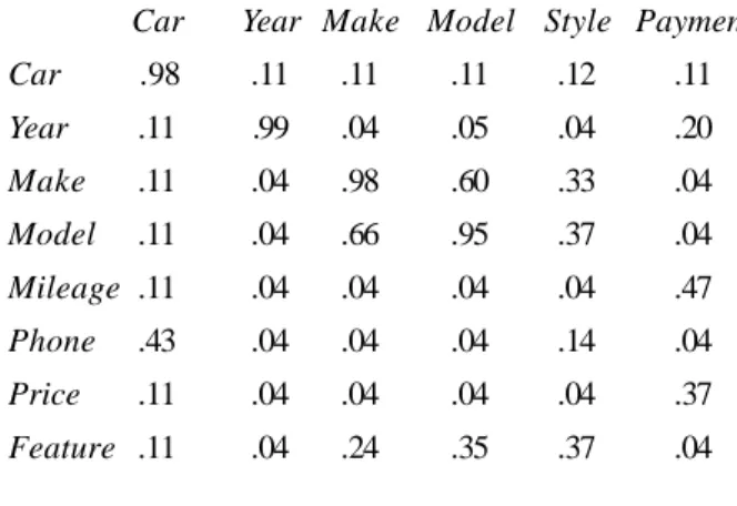
Although we would like to study more sophisticated combinations in the future, including the possibility of using machine learning to provide an appropriate decision rule, we currently use a simple average over the confidence values for each applicable attribute pair. Figure 5 shows the resulting combined matrix for our sample car-ads application.
Car Year Make Model Style Payment
Car .98 .11 .11 .11 .12 .11
Year .11 .99 .04 .05 .04 .20
Make .11 .04 .98 .60 .33 .04
Model .11 .04 .66 .95 .37 .04
Mileage .11 .04 .04 .04 .04 .47
Phone .43 .04 .04 .04 .14 .04
Price .11 .04 .04 .04 .04 .37
Feature .11 .04 .24 .35 .37 .04
Figure 5: Combined Matrix
3 Structure
One more facet of metadata that provides a clue about which attributes to match is structure. If the same relationships among source objects are found to exist among target objects, we have more confidence that we have correctly matched source and target structure than we do if we do not find matching source and target structure.
6 These decision trees can be found in a technical report available at
We can represent the structure of both source and target schemes as graphs. Nodes of the graph are object sets, and edges of the graph are relationship sets.7 Figure 6, for example, shows a target scheme graph (Figure 6(a)), a source scheme graph (Figure 6(b)), and a second source scheme graph (Figure 6(c)). In a scheme graph we denote object sets as boxes and relationship sets as lines connecting boxes. Dotted boxes are for lexical object sets, and solid boxes are for nonlexical object sets. Car is thus a nonlexical object set in Figure 6 and Year is a lexical object set. Lines with arrowheads denote functional relationship sets - For each Car there is only one Year, one Make, and one Model. Lines without arrowheads denote nonfunctional relationship sets - for each Car in Figure 6(a) there are many Features (e.g., A/C, Automatic
Transmission, ...), each of which may be applicable for many cars, and there may be more than one Phone for contacting the seller, who in turn may be selling many cars. An “O” near a connection between an object set and a relationship set denotes that objects in the object set may participate optionally in the relationship set. Thus, in Figure 6(b) a
BodyStyle may or may not have an Extension.
As an example of how structure helps resolve attribute matching, consider Extension in Figure 6. In the target (Figure 6(a)), Extension represents the extension for a phone number, whereas in the first source (Figure 6(b)), Extension represents the extended length of a cab for a truck or the extended length of the body for a sport utility vehicle (SUV). Observe that by checking the facets we have discussed so far, we would likely consider Extension in the two schemes to be a match. (1) The name is identical, so the terminological-relationship test would declare high confidence for a match. (2) The data values may be close to the same (e.g. extension 24 for a phone and a 24-inch extension for an SUV), so tests for both the data-value characteristics and the expected values would likely declare high confidence in a match. However, we can see by the structure of the graph, that they should not match. Extension for Phone should only match Extension for Body Style if Phone matches
Body Style, which should have extremely low confidence.
In the second source, Extension appears twice, once for
Phone and once for Body Style. Here we should be able to
sort out which Extension matches and which does not match by a structural comparison.
With this in mind, we defined our structure test as follows. We identified a list of structure-related features we could measure for a potential match between a target object set T and a source object set S. Most of these structure-related features involve an object set T’ in the target adjacent to T. For the relationship set linking T and
T’, we use these structure-related features to find the best
corresponding relationship set or chain of relationship sets forming a path in the source. To do so, we consider each
7 Most relationship sets are binary, and thus connect two object
sets, but n-ary relationship sets which connect three or more object sets are possible. Scheme graphs are thus actually hypergraphs.
Year
Make
Model
Mileage
Feature
Price
Phone
Extension
Car
(a) Target Scheme
Year
Make
Model
Body Style
SMRP
Number of
Doors
Extension
Car
(b) Source Scheme
(c) Second Source Scheme
Year
Make
Model
Phone
Car
Body Style
SMRP
Number of
Doors
Extension
Extension
object set S’ in the source that has a potential match with T’ and compute a score by taking the product of all the measures of the structure-related features. We then select the highest score as the best corresponding path for the
T-T’ relationship set. After finding this highest score for every
adjacent object set T’ of T, we take the average of these highest scores as the structural confidence measure for the match between T and S.
We now list the structure-related features we used. We describe each feature generically and then provide, parenthetically, our way of obtaining a measure for the feature. As part of explaining our way of obtaining a measure, we give as an example the measure for matching
Extension in the target in Figure 6(a) with Extension in the
source in Figure 6(b). Observe that the only adjacent object set to Extension in the target is Phone. Thus, in the computation, we match Phone in Figure 6(a) with each object set in the source in Figure 6(b) and compute the structure score. As it turns out, the highest of these scores is obtained when Phone matches with Car. Thus, in our examples we let T be Extension in the target, T’ be Phone in the target, S be Extension in the source, and S’ be Car in the source.
Importance Feature Object sets with more incident relationship sets are considered to be more important than object sets with fewer incident relationship sets. Target object set T and source object set S are more likely to match if their importance factor is about the same. (For either a target or source object set X, let the importance factor If (X) be # incident / Max #
incident, where # incident is the number of incident
relationship sets on X and Max # incident is the largest number of incident relationship sets in the entire scheme graph for X. Then, compute the
Importance Feature as 1 - IIf (T)-If (S) I. This value is higher when T and S have similar importance in their respective scheme graphs. For our example, since the source in Figure 6(a) has a maximum of 7 incident relationship sets on any of its object sets and since
Extension has one incident relationship set, the
importance factor for T, If (T), is 1I 7 = .14. Similarly, If (S) is 1I 5 = .20. Thus, the value for the importance feature is 1 - I .14 - .20 I = .94.)
Match Score This is the confidence value of a match between target object set T and source object set S based on all independent facets. (We compute this score as the average of the confidence values for all the independent facets for T and S. For our example, we assume that the Extension-Extension score is computed to be .98. This value is consistent with the highest values in Figure 5.)
Match Score of Adjacent Object Sets This is the confidence value of a match between target object set T’ and
source object set S’ based on all independent facets. (We compute this score as the average of the confidence values for all the independent facets for
T’ and S’. For our example, we assume that the Car score is computed to be .43, the value for Phone-Car in Figure 5.)
Distance Feature If the number of relationship-set edges along corresponding paths in the target and source are the same, our confidence should increase. (For given object sets T, T’, S, and S’, we compute this as (MAX_DIST - min(distance - 1;MAX_DIST)) I
MAX_DIST, where the “1” represents the one
relationship set connecting T and T’, distance is the number of relationship sets along the shortest path connecting S and T’ in the source scheme graph, and
MAX_DIST is a user supplied threshold specifying
the maximum distance we will consider before saying that two source object sets are not close enough to be of interest for this measurement. For our experiments, we let MAX_DIST = 5. For our example
distance = 2, since there are two relationship sets
along the path from Extension to Car in the source. Hence, we have (5 - min(2 - 1; 5)) I 5 = .80.)
Function Feature If the functional characteristics along corresponding paths in the target and source are the same, our confidence should increase. (We compare the functional characteristics of the relationship set connecting T and T’ with the functional characteristics of the relationship sets along a path connecting S and S’. If the functional characteristics of the T-T’ relationship set are the same as the functional characteristics of a path, we score the path as 1.0 and otherwise score the path as F, a user-supplied value, which we set at 0.8 for our experiments. If more than one path exists in the source, we compute the score for each and take the highest. For our example, the relationship set Phone-Extension in the target has no function in either direction. In the source, however, there is a function from Car to Body Style and from
Body Style to Extension and thus, in the join, there is
a function from Car to Extension. Since the functional characteristics do not match, the value for this measure is 0.8.)
the path as O, a user-supplied value, which we set at 0.8 for our experiments. If more than one path exists in the source, we compute the score for each and take the highest. For our example, Phone is optional for the relationship set Phone-Extension in the target. In the source since Body Style is optional in the relationship between Body Style and Extension, Car is optional in the join of the relationships from Car to
Body Style and from Body Style to Extension. Thus,
the optionality characteristics are the same, and hence, the value for this measure is 1.0.)
Leaf-Node Feature If corresponding object sets of corresponding paths in the target and source are either both leaf nodes or both nonleaf nodes in the scheme graph, our confidence should increase. (For this measure, we determine whether T’ and S’ are either both leaf nodes — have one incident relationship-set edge, or are both nonleaf nodes — have more than one incident relationship-set edge. If so, the score is 1.0, and otherwise is N, a user-supplied value, which we set at 0.3 for our experiments. Since neither Phone nor Car is a leaf node in our example, the score is 1.0.)
Lexical Feature If corresponding object sets of corresponding paths in the target and source are either both lexical or both nonlexical, our confidence should increase. (For this measure, we determine whether T’ and S’ are either both lexical or both nonlexical. If so, the score is 1.0, and otherwise is L, a user supplied value, which we set at 0.2 for our experiments. Since Phone is lexical and Car is nonlexical in our example, the score is 0.2.)
Finishing our example, we take the product of all the scores: Importance (.94) x Match (.98) x Adjacent Match (.43) x Distance (.80) x Functional (.80) x Optional (1.00) x Leaf-Node (1.00) x Lexical (.20) = .05. Since there are no other object sets besides Phone for Extension in the target, we take this score as the (degenerate) average score for the structure match between Extension in the target scheme in Figure 6(a) and Extension in the source scheme in Figure 6(b). By way of comparison, the structure score for the match between Extension in the target (Figure 6(a)) and Extension attached to Phone in the second source scheme (Figure 6(c)) is .93 (= Importance (1 - I 1I 7 - 1I 6 I = .97) x Match (.98) x Adjacent Match (.98)
x Distance ((5 - min (1-1,5))I 5 = 1.00) x Functional (1.00) x Optional (1.00) x Leaf-Node (1.00) x Lexical (1.00)). Further, by way of comparison, for the match between Extension in the target (Figure 6(a)) and Extension attached to Body
Style in the second source scheme (Figure 6(c)), the best
structure score arises from the Phone-Phone match for the adjacent object set instead of the Phone-Car match.
This score is .56 (= Importance (1 - I1 I 7- 1 I 6I = .97) x
Match (.98) x Adjacent Match (.98) x Distance ((5 - min(3
- 1, 5)) I 5 = .60) x Functional (1.00) x Optimal (1.00) x
Leaf-Node (1.00) x Lexical (1.00)). These scores correspond to our intuitive notion of “structural goodness.” Figure 7 shows the results of applying the structural rule for our car-ads application.
4 Settling Attribute Matches
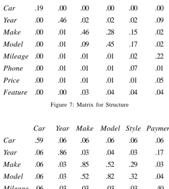
Before settling matching pairs, we produce one more matrix, which is the average over all the confidence values. Figure 8 shows this matrix.
We settle matching pairs by the algorithm in Figure 9, which is greedy (selects the highest confidence value first) and is an injective assignment algorithm (allows at most one match for any row or column). When we run this algorithm on the matrix in Figure 5 with a threshold value of 0.5, we obtain the final matrix in Figure 10. Observe that even though “Make-Model” pairs have values exceeding the threshold, the injective assignment constraint eliminates these matches because they are precluded by the “Make-Make” and “Model-Model” matches. Thus, the final matching pairs are {Car, Car}, {Year, Year}, {Make, Make}, and {Model, Model}, as they should be.
Car Year Make Model Style Payment
Car .19 .00 .00 .00 .00 .00
Year .00 .46 .02 .02 .02 .09
Make .00 .01 .46 .28 .15 .02
Model .00 .01 .09 .45 .17 .02
Mileage .00 .01 .01 .01 .02 .22
Phone .00 .01 .01 .01 .07 .01
Price .00 .01 .01 .01 .01 .05
Feature .00 .00 .03 .04 .04 .04
Figure 7: Matrix for Structure
Car Year Make Model Style Payment
Car .59 .06 .06 .06 .06 .06
Year .06 .86 .03 .04 .03 .17
Make .06 .03 .85 .52 .29 .03
Model .06 .03 .52 .82 .32 .04
Mileage .06 .03 .03 .03 .03 .40
Phone .22 .03 .03 .03 .12 .03
Price .06 .03 .03 .03 .03 .29
Feature .06 .03 .19 .27 .29 .03
5 Experimental Results
In addition to our sample application presented here, we applied our method to six other car-ads sites found on the Web and obtained similar results. Over all test cases, the process correctly matched 31 of 32 of the direct matches, for a recall value of 97%. The one false negative was the pair Mileage-Miles. WordNet does not recognize these words as being synonyms; it converts the plural Miles into the singular Mile and then attempts to match Mileage with
Mile, which are not related. The expected-value measure
also runs into trouble because the format in which the values appear was not anticipated by the regular expressions for mileage.
Car Year Make Model Style Payment
Car 1 0 0 0 0 0
Year 0 1 0 0 0 0
Make 0 0 1 0 0 0
Model 0 0 0 1 0 0
Mileage 0 0 0 0 .03 .40
Phone 0 0 0 0 .12 .03
Price 0 0 0 0 .03 .29
Feature 0 0 0 0 .29 .03
Figure 10: Final Matrix
There were 2 false matches among a potential of 376 false matches, resulting in a precision value of 31I (31+2) = 94%. In one test case Feature matched Color, and in another Feature matched Body Type. In our car-ads ontology, both colors and body types are special kinds of features, and thus the match was not entirely wrong - just not exact. In future work we intend to resolve partial matches such as these. To do so, we will need to recognize the possibility of a partial match, and thus these false matches will potentially become very useful.
By way of comparison, we ran each individual independent-facet matrix alone through the settling
algorithm. In these tests, the settling process found only 72 of the 82 direct matches (29 of 32 for WordNet, 21 of 25 applicable matches for value characteristics, and 22 of 25 applicable matches for expected values). This reduces the overall recall from 97% to 88%. The settling process also found 19 false matches (4 for WordNet, 9 for value characteristics, and 6 for expected values.) This reduces the overall precision from 94% to 79%. The structure facet is not independent, but it too suffers a degradation (as we show in the next section) when we use it with only one of the other facets as opposed to all of them together. These results suggest that the multifaceted approach proposed here is likely to be better than any single-faceted approach.
6 Limited Facets
To further test the approach we propose here, we considered three additional applications - music CDs, genealogy, and real estate. We found Web sites for these applications and faithfully converted the information for each site into a scheme graph. By “faithfully” we mean that we preserved the original vocabulary of the site as well as the implied constraints and structure. Altogether, we obtained 4 scheme graphs for music CDs, 4 for genealogy, and 5 for real estate. As an example, Figure 11 shows the four scheme graphs for music CDs.
For these applications, we only applied our terminological and structural facets. We did not extract values, and we did not develop recognition expressions for expected values for each of the object sets. Although this limitation prevents us from testing for data-value characteristics and for expected values, we were still able to apply our technique. This situation is typical of many real-world situations where we may have limited information. For testing these applications, we decided to let any one of the scheme graphs for an application be the target and let any other scheme graph be the source. Because our tests are nearly symmetrical, we decided not to test any target-source pair also as a source-target pair, with the chosen target as the source and the chosen source as the Input: a matrix M of confidence values, and a threshold T.
Output: a set of matching attribute pairs.
While there is an unsettled confidence value in M greater than T Find the largest unsettled confidence value V in M; Settle V by setting it to 1;
Mark V as being settled;
For each unsettled confidence value W in the rows and columns of V Settle W by setting it to 0;
Mark W as being settled;
Output the settled attribute pairs whose value is 1;
target. We also decided not to test any single scheme graph as both the target and the source. For the music CD schemes in Figure 11, for example, we tested the following target-source pairs: AllMusic-Amazon, AllMusic-CDNow, AllMusic-MovieMusic, CDNow-Amazon, MovieMusic-CDNow-Amazon, MovieMusic-CDNow.
For comparison, we also retested our car-ads applications using only terminological and structural facets. For these tests, we used the same single target we had already chosen for each of the seven sources. Altogether we ran 29 tests (7 for car-ads, 6 for music CDs, 6 for genealogy, and 10 for real estate).
(a) AllMusic Scheme
Death Date
Death Place Birth Place
Birth Date
Real Name
Name
Genre
Style
Instrument
Biography
Author
Text Artist
Role
Album Album Title
Date of Release
Rating Genre
Style
Time
Review
Text
Author Track
Composer Time Title
Label
Medium
Year
Catalog Number Release
Figure 11: Scheme Graphs for Music CDs
(b) Amazon Scheme
List Price Artist
Title
Our Price
Number of Discs
Average Customer Review
Number of Reviews Availability
Release Date
Original Release Date Audio CD
Sample
Track
Track Name
Rating
Title
Reviewer Date
Text Customer Review
Editorial Review
Company Author
Text
(c) CDNow Scheme List Price
All Music Guide Pick (Price)
Date Album
Length
Label
Genre
Category Artist
Image
CD
Production Credit
Role Name
Performer
Part Name
Title
Composer
Time
Sample Track
(d) Movie Music Scheme
Genre Year
Composer
Title
Image
Label
Rating
Track
Sample
Title Favorate Track
Review Text
Date
Reviewer Rating Sound Track
For each test, we used the WordNet rule in Figure 1, the structure rule described in Section 3 (with the same user-supplied values), and the same threshold value, 0.5. Table 1 shows the results - giving for each application and over all applications together (1) the number of matches N determined by a human expert, (2) the number of correct matches C selected by the process described in this paper, (3) the number of incorrect I matches selected by our process, (4) the recall ratio, R = C I N, which we express as a
percentage, (5) the precision ratio, P = C I (C + I), which we
express as a percentage, and the F-measure, 2 I (1 I R + 1 I P
), a standard measure for recall and precision together [24], which we also express as a percentage. Over all these test cases, the process correctly matched 210 of the 268 direct matches, for a recall ratio of 210/268 = 78%. There were 121 false matches among a potential of 13,347 false matches, resulting in a precision ratio of 210I (210+121) = 63%.
Generally, we observed that limiting the facets to just terminological relationships (based on WordNet) and structure, the results are not as good as the results using all the facets. In particular, we observed that the recall for car-ads dropped from 97% to 91% and that the precision dropped from 94% to 88%. We also observed that both recall and precision were lower for the other applications when compared to the car-ads application. In the following paragraphs we specically discuss the problems that arose and suggest some possible solutions.
The false matches are those our process matched that should not have been matched. They generally fall into three categories: (1) matches that would probably have been avoided if we had been able to consider values (51%), (2) those that are actually correct but which we counted as being incorrect because they only partially match (26%), and (3) those that would need enhancements to the process to be properly eliminated (23%).
- Examples of matches that would probably have been avoided if we had been able to consider values include
Year-Time from music CDs, Title-Given_Name from
genealogy, and Number_of_Floors-Floor_Size from real estate. In all cases regular expressions looking for
expected values would have been able to distinguish values for these pairs, and further consideration of value characteristics would likely only enhance the differences.
- An example of a partial match is Author-Reviewer in the
music-CD application. The problem here is that in AllMusic (Figure 11(a)) there is only one type of reviewer, whereas in Amazon (Figure 11(b)) there are two types of reviewers - customer reviewers and editorial reviewers. Thus, there is really no direct match, so we declared Author-Reviewer as an incorrect match. What is really needed, however, is to accept the partial match Author-Reviewer and the partial match Reviewer-Reviewer and then realize that we actually need a virtual object set computed as the union of Author and Reviewer in Figure 11(b) to match with Reviewer in Figure 11(a). This is an example of an indirect match, which we leave for future work.
- An example of the additional kinds of information needed is terminological understanding of phrases — WordNet does not do well with the various kinds of dates, such as christening dates, burial dates, and marriage dates, found in the genealogy application. Another example is terminological understanding of contextual relationships — Date attached to CD in Figure 11(c) should not match
Date attached to Review in Figure 11(d).
The missed matches are those our process should have matched, but failed to match. They generally fall into three categories: (1) matches that require specialized or jargon vocabulary (43%), (2) those that are actually correct but were missed because they were precluded by other correct matches (40%), and (3) those that would need enhancements to the process to be properly accepted (17%).
- Examples of synonyms that should have been recognized, but were not because they are only synonyms in a special application include Property and Listing in the real estate application and Title and Album in the music-CD application. Achronyms and abbreviations also fall into this category. We are likely to need specialized dictionaries to resolve these difficulties.
Application Number of Number Number Recall Precision F-Measure
Matches Correct Incorrect % % %
Car Advertisements 32 29 4 91% 88% 89%
Music CDs 67 52 35 78% 60% 68%
Genealogy 47 42 12 89% 78% 83%
Real Estate 122 87 70 71% 55% 62%
All Applications 268 210 121 78% 63% 70%
- Partial matches can preclude declared direct matches. What
we really want, however, is to be able to recognize and sort out all the partial matches so that we can obtain virtual object sets containing all the correct objects and only the correct objects. This problem is nontrivial, sometimes even for human experts, and we may have to accept subsets and supersets in our results.
- An example of the additional kinds of information needed is terminological understanding about how to disambiguate relationship-set names — Place in one of the genealogical schemes could only be distinguished by its connecting relationship — set names: birth,
christening, death, and burial. Another example is text
analysis for classification of descriptive paragraphs—
Text in one of the real-estate schemes should have
matched with Description in another.
7 Conclusion
We presented a framework for discovering direct matches between sets of source and target attributes. In our framework, multiple facets each contribute in a combined way to produce a final set of matches. Facets considered include terminological relationships such as synonyms and hypernyms, data-value characteristics such as variances and string lengths, expected values as declared by target regular-expression recognizers, and structural characteristics based on scheme graphs.
The results are encouraging and show that the multifaceted approach to exploiting metadata for attribute matching has promise. When we used all four facets for our car-ads tests we obtained recall and precision results above 90%. Recall and precision dropped off when we reduced the number of facets to either single independent facets or to our terminological facet followed by our structural test.
Analyzing false matches and missed matches led to a number of ideas for future work. (1) We should recognize and resolve partial matches by generating virtual object sets and virtual relationship sets in the source that directly match object and relationship sets in the target. (2) We should consider ways to better do terminological relationship matching so that we can do phrases in the context of relationship sets and adjacent object sets. (3) We should expand our multifaceted approach to include classification of text, both to match paragraphs of text that are values of target and source attributes and to add an additional facet that considers descriptive dictionary information. (4) We should gather sufficient training data so that we can apply machine learning to generate rules for structure and for determining thresholds. (5) We should gather more test cases for our current applications, and we should investigate a broader array of applications.
Although we have accomplished much, as is usually the case in these types of scientic investigations, there is much more to be done.
References
[1] J. Larson, S. Navathe, and R. Elmasri. A theory of attribute equivalence in databases with application to schema integration. IEEE Transactions on Software
Engineering, 15(4), 1989.
[2] W.-S. Li and C. Clifton. Semantic integration in heterogeneous databases using neural networks. In
Proceedings of the 20th Very Large Data Base Conference, Santiago, Chile, 1994.
[3] E.H.C. Chua, R.H.L.Chiang, and E-P. Lim. Instance-based attribute identication in database integration. In
Proceedings of the 8th Workshop on Information Technologies and Systems (WITS’98), Helsinki,
Finland, December 1998.
[4] M. Garcia-Solaco, F. Slator, and M. Castellanos. A structure based schema integration methodology. In
Proceedings of the 11th International Conference on Data Engineering (ICDE’95), pages 505{512,
Taipei, Taiwan, 1995.
[5] J. Fowler, B. Perry, M. Nodine, and B. Bargmeyer. Agent-based semantic interoperability in InfoSleuth.
SIGMOD Record, 28(1):60{67, March 1999.
[6] S. Hayne and S. Ram. Multi-user view integration system (MUVIS): An expert system for view integration. In
Proceedings of the 6th International Conference on Data Engineering, pages 402{409, February 1990.
[7] S. Bergamaschi, S. Castano, and M. Vincini. Semantic integration of semistructured and structured data sources. SIGMOD Record, 28(1):54{59, March 1999. [8] S. Castano and V. De Antonellis. Semantic dictionary
design for database interoperability. In Proceedings
of 1997 IEEE International Conference on Data Engineering (ICDE’97), pages 43{54, Birmingham,
United Kingdom, April 1997.
[9] V. Kashyap and A. Sheth. Semantic and schematic similarities between database objects: A context-based approach. The VLDB Journal, 5:276{304, 1996. [10] V. Kashyap and A. Sheth. Semantic heterogeneity in
global information systems: The role of metadata, context and ontologies. In M. Papazoglou and G. Schlageter, editors, Cooperative Information Systems:
Current Trends and Directions, pages 139{178, 1998.
[11] S. Castano, V. De Antonellis, M.G. Fugini, and B. Pernici. Conceptual schema analysis: Techniques and applications. ACM Transactions on Database
[12] J. Biskup and D.W. Embley. Extracting information from heterogeneous information sources using ontologically specied target views. Information
Systems, 28(3) 29-54, 2003.
[13] D.W. Embley, B.D. Kurtz, and S.N. Woodeld.
Object-oriented Systems Analysis: A Model-Driven Approach. Prentice Hall, Englewood Cliffs, New
Jersey, 1992.
[14] D.W. Embley, D.M. Campbell, Y.S. Jiang, S.W. Liddle, D.W. Lonsdale, Y.-K. Ng, and R.D. Smith. Conceptual-model-based data extraction from multiple-record Web pages. Data & Knowledge Engineering, 31(3):227{251, November 1999.
[15] D.W. Embley and M. Xu. Relational database reverse engineering: A model-centric, transformational, interactive approach formalized in model theory. In
DEXA’97 Workshop Proceedings, pages 372{377,
Toulouse, France, September 1997. IEEE Computer Society Press.
[16] S.H. Yau. Automating the extraction of data behind web forms. Technical report, Brigham Young University, Provo, Utah, 2001. http:// www.deg.byu.edu.
[17] N. Ashish and C. Knoblock. Wrapper generation for semi-structured internet sources. SIGMOD Record, 26(4):8{15, December 1997.
[18] P.B. Golgher, A.H.F. Laender, A.S. da Silva, and Ribeiro-Neto. An example-based environment for wrapper generation. In S.W. Liddle, H.C. Mayr, and B. Thalheim, editors, Proceedings of the 2nd International
Conference on the World-Wide Web and Conceptual Modeling, Lecture Notes in Computer Science, 1921,
pages 152{164, Salt Lake City, Utah, October 2000. [19] J. Hammer, H. Garcia-Molina, S. Nestorov, R. Yerneni,
M. Breunig, and V. Vassalos. Template-based wrappers in the TSIMMIS system. In Proceedings of 1997 ACM
SIGMOD International Conference on Management of Data, pages 532{535, Tucson, Arizona, May 1997.
[20] G.A. Miller. WordNet: A lexical database for English.
Communications of the ACM, 38(11):39{41, November 1995.
[21] C. Fellbaum. WordNet: An Electronic Lexical Database. MIT Press, Cambridge, Massachussets, 1998. [22] J.R. Quinlan. C4.5: Programs for Machine Learning.
Morgan Kaufmann, San Mateo, California, 1993. [23] S. Castano and V. De Antonellis. ARTEMIS: Analysis
and reconciliation tool environment for multiple information sources. In Proceedings of the Convegno
Nazionale Sistemi di Basi di Dati Evolute (SEBD’99),
pages 341{356, Como, Italy, June 1999. [24] R. Baeza -Yates and B. Ribeiro-Neto. Modern
Information Retrieval. AddisonWesley, Menlo Park,