ISSN 0101-8205 www.scielo.br/cam
Block linear method for large scale
Sylvester equations
MARLLINY MONSALVE
Scientific Computing Center, Departamento de Computación, Facultad de Ciencias Universidad Central de Venezuela, Ap. 47002, Caracas 1041-A, Venezuela
E-mail: [email protected]
Abstract. We present and analyze a new iterative scheme for large-scale solution of the
well-known Sylvester equation. The proposed scheme is based on fixed point iteration approach
and can make good use of the recently developed methods for solving block linear systems.
It is shown mathematically that the iterative process converges under some assumptions on the
coefficient matrices. Results on our numerical experiments with large-scale matrices are quite
encouraging. In particular, the method compares favorably with the other block methods and a
recently proposed method for Sylvester equation based on low-rank approximation of the right
hand side matrixC.
Mathematical subject classification: 65J10, 65F10, 15A24.
Key words: Sylvester equation, block linear systems, iterative methods.
1 Introduction
In this paper, we present a new block algorithm for solving the Sylvester matrix equation (SE):
A X−X B =C, (1)
whereA,B, andCare given matrices of dimensionsn,p, andn×p, respectively and the matrix X of dimensionn×pneeds to be found.
It is well-known (see [6] and the original paper of Sylvester [16]) that the equa-tion (1) has a unique soluequa-tion if and only ifAandBdo not have an eigenvalue in
common. The necessity of solving this equation arises in a wide variety of practi-cal applications, including control systems design and analysis [4, 6], numeripracti-cal solutions of differential equations, including boundary value problems [2, 8].
Because of its importance, the problem has been well studied in the literature and there now exist many methods for its solutions. An account of these meth-ods can be found in the recent book by Datta [6]. In theory, the problem can be reduced to a linear system problem whose system matrix is a Kronecker product matrix of large dimension. The Kronecker-product approach is not numerically viable even for a small and dense system. For details see again the book by Datta [6]. The best-known and very widely used numerical method for small and dense problems is the Hessenberg-Schur method by Golub, Nash, and Van Loan [9]. The method is based on reduction of the largest of two matrices to Hessenberg form and the other to real Schur form. The Hessenberg-Schur method is an effi-cient implementation of the Bartels-Stewart method [1] proposed earlier, based on the reductions of both matrices to Schur forms. Unfortunately, these methods are not practical for large and sparse problems.
In this paper, we propose a new iterative scheme based on fixed point iteration. The scheme requires solution of a linear systems with multiple right-hand sides at each iteration, which can be solved by using block Krylov subspace methods for linear systems (see Brezinski [3], Saad [15]). Our method method does not require solution of a low-dimensional Sylvester equation at every iteration. The results of our numerical experiments show that the proposed method works quite well for large-scale problems and is quite competitive with the other existing competing methods. Mathematical results on the convergence of our iterative scheme is also provided in the paper.
2 Methods based on SE and block linear systems
The main idea to solve the SE is to write this equation as a block linear system and then use some suitable iterative scheme. This can be accomplished by the following change of variable: A X = Z where Z =C +X B. This possibility generates the iterative method:
Algorithm 1 Using: A X =Z 1: GivenX0∈Rn×p
2: ComputeZ0=C+X0B
3: fork =0,1,· · · until convergencedo 4: Solve A Xk+1=Zk
5: SetZk+1=C+Xk+1B 6: end for
Notice that, the method requires the solution of one block linear system and one matrix-matrix product per iteration. The matrix of coefficients of the inter-nal system is of dimensionn, therefore from a computational-cost point of view ifn< pit is convenient to use Algorithm 1 as described, but ifn> pit is con-venient to transpose the Sylvester equation, and then apply Algorithm 1. To be precise, whenn > psolving−BTXT +XTAT =CT, instead of (1), should be
Our next result establishes convergence under an additional hypothesis on the matrices A and B. This additional hypothesis is sufficient to guarantee also the existence of a unique solution, and as far as we know, it is the classical hypothesis assumed when dealing with iterative schemes that are not related to Krylov subspace methods, see [13].
Theorem 2.1. LetA∈Rn×n,B ∈Rp×p,C ∈Rn×pand let.be an induced
norm. If A−1B < 1 then equation (1) has a unique solution, and the sequence{Xk}k≥0generated by Algorithm1converges q-linearly to the solution.
Proof. Letλi(A)be the eigenvalues of Afor 1≤ i ≤ nand letλj(B)be the
eigenvalues of B for 1 ≤ j ≤ p. Since A ≥ |λi(A)|for anyi and for any
induced norm we haveA−1 ≥max1
≤i≤n|λi(A−1)|and thus,
1 A−1 ≤
1
max1≤i≤n|λi(A−1)|
= min
1≤i≤n|λi(A)|. (2)
On the other hand,A−1B<1⇒ B< 1
A−1,now using (2) we obtain,
max 1≤j≤p
|λj(B)|< min
1≤i≤n|λi(A)| ⇒σ (A)∩σ (B)= ∅. (3)
From (3) we conclude, that equation (1) has a unique solution since the spectra of AandBare disjoint.
For the convergence we proceed as follows. From Algorithm 1 we obtain that Xk = A−1(C+Xk−1B)and from SE we know that X = A−1(C +X B). Combining these two equations it follows that
X−Xk = A−1(X−Xk−1)B, (4) and so,
X−Xk =(A−1)k(X −X0)(B)k.
Therefore
X−Xk ≤(A−1B)k(X−X0).
Since A−1B < 1 then the sequence X
k converges to X when k tends to
on equation (4) we have that
Ek ≤ A−1BEk−1, since A−1B < 1 then the sequence X
k converges q-linearly to the the
solution.
Notice that if no information is available about A−1 orB−1 then A andB could be of help to decide whether it is convenient to solve (1) or its transpose to increase the possibility of convergence. For example, if A is much larger thanB, then the conditionA−1B<1 is likely to be satisfied for convergence when solving (1). Similarly, the transpose approach should be preferred whenBis much larger thanA. Notice also that, if we want to solve SE with B = A(or B = AT), then Theorem 2.1 does not guarantee convergence, sinceAA−1 =cond(A)≥1.Unfortunately, this includes the well-know Lyapunov equation.
For the proposed algorithm, the residual matrix at iteration k is defined as Rk =C−(A Xk −XkB). This expression involves a high computational cost,
since it require two matrix-matrix products per iteration. The following result provides an equivalent and less expensive way to calculate the residual.
Theorem 2.2. Let {Xk}k≥0 be the sequence generated by Algorithm 1. The
following expressions for the residual matrix are equivalent:
a) Rk =C−(A Xk−XkB)=C+XkB−A Xk.
b) Rk =Zk−Zk−1. c) Rk =(Xk−Xk−1)B.
Proof. The residual is given by Rk =C+XkB−A Xk and from Algorithm 1
we have that Zk =C+XkBandA Xk = Zk−1. Therefore
Rk = Zk−Zk−1. (5)
On the other hand, substituting Zk from Algorithm 1 in (5) we obtain Rk =
C+XkB−(C+Xk−1B). Therefore
Equation (5) provides a less expensive form to calculate the residual since it does not involve matrix-matrix products. Finally from (6) we obtain the follow-ing corollary which yields a more convenient stoppfollow-ing criterion.
Corollary 2.1. Let {Xk}k≥0 be the sequence generated by Algorithm 1. If Xk−Xk−1 →0, thenRk →0.
Finally, the following result establishes a bound that relates the norm of the residual and the norm of the error.
Theorem 2.3. Let {Xk}k≥0 be the sequence generated by Algorithm 1. The
norm of the residual matrix satisfies that:
Rk ≤(A + B)Ek (7)
Proof. Rk =C−(A Xk−XkB)= A X−X B−A Xk+XkB = A(X−Xk)−
(X−Xk)B= AEk −EkB.Therefore
Rk = AEk−EkB ≤(A + B)Ek
3 Numerical results
In this section we present preliminary numerical experiments to illustrate the performance of the new proposed algorithm. For solving the internal block linear systems for this algorithm we use the block SOR scheme (BSOR), the non-Hermitian block steepest descent method (BSD) and the block minimal residual iteration (BMR) fully described in [3]. For the proposed algorithm, we will only present the combination that better results generated in CPU time. For each experiment, we will indicate which method was used to solve the internal block linear system.
We compare the new proposed algorithm with the following methods for solv-ing SE:
iteration of orderm p 2, wheremis the restart value. These internal SE are solved using the algorithm proposed by Golub, Nash and Van Loan in [9]. The BAS(m) and BGS( m) can only be used when n>> p. Whenn< p we can always transpose SE and then apply the same techniques.
• Galerkin method for Sylvester equation (GMSE(m)) and the restarted minimal projected residual algorithm (RMPR(m)) proposed and fully de- scribed in [11]. These methods, as well as BAS(m) and BGM( m), are based on Krylov subspace methods and solve a small SE per iteration of orderm2. The internal SE is written as a linear system of equation of order
m2that is solved using direct methods, but the operation count for these algorithms ismnp flops. GMSE(m) and RMPR( m) can be used for any values ofnandp.
• Arnoldi method for low-rank approximate solution to the Sylvester equa-tion (LRASE(k,m)) proposed and fully described in [14]. The parameter k is a small value required by the algorithm, andmis the restart value. This method can be used for any values ofnandp. In all our experiment, we prove for 1≤k ≤5 and we report the best result.
In our tests we use matrices from the Harwell-Boeing collection and also some sparse matrices from the Matlab gallery, and for these matrices the inequalities of Theorem 2.1 hold, therefore convergence is guaranteed for the new proposed algorithm. In all cases, the entries of the solution matrix X arexi j = f(xi,yj)
where: xi = i hn, yj = j hp for 0 ≤ i ≤ n, 0 ≤ j ≤ p, hn = 1/(n+1),
hp = 1/(p +1) and f(x,y) = xex ysin(πx)sin(πy). This is a typical test
function that appears in several works, see e.g. [11, 10]. We stop the process when
X−Xk = Ek ≤10−8,
or when 2500 external iterations are reached. The initial iterate, X0, is the null matrix. To stop the iterative methods for the internal block linear systems we use the norm of the residual. To be precise, we stop the internal iterations of Algorithm 1 when A Xk+1−Zk ≤10−2. The experiments were run in a
7.0. In examples 3.1–3.4 we compare the performance of Algorithm 1 with other methods. In these examples we report number of iterations (Iter), CPU time, norm of the residual (Residual) and norm of the absolute error (Error). In example 3.5 we compare the different equivalent expressions for computing the residual norm.
We used the following notation for characterizing the different finalization states of the experiments, “–” means that the algorithm accomplished the max-imum number of external iterations, “s” implies that the used method produced stagnation problems and “**” means that the memory requirements of the algo-rithm could not be supported by Matlab.
Example 3.1. In this example n < p and n is a small value. The ma-trix B is the matrix Hor__131 of the Harwell-Boeing collection with p = 434, and A is a sparse matrix of order n generated with the Matlab function
gallery(’wathen’,nx,ny)wheren=3∗nx∗ny+2∗nx+2∗ny+1 which returns a sparse random finite element matrix.
Methods Iter CPU time Residual Error BAS(4) 15 2.20 1.21e-008 7.89e-009 BGS(4) 2 0.81 4.11e-012 4.06e-013 GMSE(4) 104 16.26 1.02e-007 9.19e-009 RMPR(4) 99 16.12 1.60e-007 7.28e-009 LRASE(1,4) 198 1.67 3.88e-008 9.86e-009 Algorithm 1 + BSOR 19 0.36 9.18e-008 5.49e-009
Table 1 – Performance of BAS(m), BGS(m), GMSE(m), RMPR(m), LRASE(k,m) and Algorithm 1 combined with BSOR for solving SE whenB=Hor__131andAis a sparse
random finite element matrix withnx =2,ny=1 andn=13.
Example 3.2. In this example,Ais the matrixorsirr_2withn=886 andBis the matrixsherman1with p=1000, both of the Harwell-Boeing collection.
Methods Iter CPU time Residual Error
BAS(4) ** ** ** **
BGS(4) ** ** ** **
GMSE(4) - 4692.6 - 0.699
RMPR(4) s s s 1.23
LRASE(1,4) - 27299.79 - 14.62 Algorithm 1 + BSOR 1567 53494.81 1.03e-007 9.95e-009
Table 2 – Performance of BAS(m), BGS(m), GMSE(m), RMPR(m), LRASE(k,m)
and Algorithm 1 combined with BSOR for solving SE when A =orsirr_2andB = sherman1.
As shown in Table 2, BAS and BGS produce storage problems. In this ex-perimentE0 =616.24, and we can observe that GMSE, RMPR and LRASE reduce the absolute error norm. RMPR produces stagnation problems while GMSE and LRASE stopped because the maximum number of external itera-tions was reached. Finally, Algorithm 1 with BSOR converges but the CPU time required is considerably higher.
Example 3.3. In this example p <n and pis a small value. The matrix Ais the matrixgre__343of the Harwell-Boeing collection withn=343, andBis a tridiagonal matrix of order p=20 given by
B =α∗tr i di ag(−1−p1h, 2−p2h2, −1+p1h) (8) with
h = 1
p+1, α = − 1
h2, and p1=100, p2=50.
This matrix has been used by several authors, see [10, 11, 14]. In this experiment we report Algorithm 1 combined with BMR.
Methods Iter CPU time Residual Error BAS(4) 12 6.70 3.70e-006 4.15e-009 BGS(4) 1 8.21 9.48e-011 1.41e-013 GMSE(4) 368 6.96 8.30e-005 9.93e-009 RMPR(4) 344 6.39 5.32e-005 8.54e-009 LRASE(1,4) 248 3.67 7.80e-006 9.73e-009 Algorithm 1 + BMR 5 0.078125 5.56e-007 6.29e-010
Table 3 – Performance of BAS(m), BGS(m), GMSE(m), RMPR(m), LRASE(k,m) and Algorithm 1 combined with BMR for solving SE when A =gre__343andB =is a
tridiagonal matrix.
almost twice the one required by LRASE. On the other hand, BGS converges in one iteration and it reduces the norm of the error more than the others, but the CPU time required by BGS is higher than the one required by the others. It is worth noticing that for this example, we use the values of p1and p2suggested in [11].
Example 3.4. In this example,Ais the matrixgre_1107withn=1107 andB is the matrixfs_760_1with p=760, both from the Harwell-Boeing collection.
Methods Iter CPU time Residual Error
BAS(4) ** ** ** **
BGS(4) ** ** ** **
GMSE(4) - 4586.23 - 2.4682
RMPR(4) s s s 2.6002
LRASE(1,3) - 28879.03 - 755.96 Algorithm 1 + BSD 636 1596.26 0.147e-002 9.58e-009
Table 4 – Performance of BAS(m), BGS(m), GMSE(m), RMPR(m), LRASE(k,m) and Algorithm 1 combined with BSD for solving SE whenA=gre_343andB=fs_760_1.
con-verges. In this experimentE0 =458.5 and we can see that GMSE and RMPR reduced the absolute error norm while LRASE increased it. Finally, we can observe that Algorithm 1 achieves convergence but Rkis much higher than
Ek.
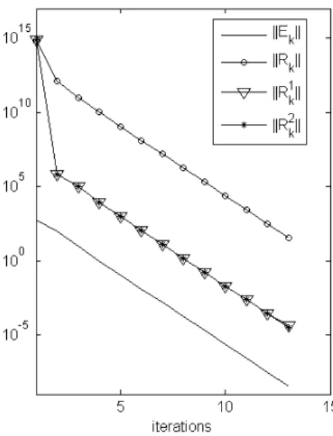
Example 3.5. In this example we want to compareEk, with the equivalent
expressions for the norm of the residual described in Theorem 2.3. These expres-sions will be denoted byRk = C −(A Xk−XkB),Rk1 = Zk−Zk−1 and R2
k = (Xk − Xk−1)B. The matrix A is the matrix fs_680_1 of the Harwell-Boeing collection and B is a sparse matrix with random entries. The dimensions of these matrices aren =680 and p =1000 respectively. We use Algorithm 1 combined with BSOR to solve SE.
Figure 1 – Comparison of Ek, Rk, R1k andRk2 when we use Algorithm 1 combined with BSOR, to solve a SE with A=fs_680_1andBhas random entries.
In Figure 1, we can see that R1
k and R2k are close to Ek during the
process, while Rk is not. In this exampleA + B = 7.19e+013 and
the behavior observed in Figure (1) agrees and illustrates (7). Finally, we can conclude that if the stopping criterion isRk ≤ tol E, it is convenient to use
work: Rk requires 2 matrix-matrix product, while R1k requires a matrix
substraction. The second reason is thatRk1is more accurate to measure the precision of the approximation generated by the proposed algorithms.
4 Concluding remarks
We propose a new iterative scheme for solving Sylvester Equations (SE). At each iteration a block linear system of equations is solved and, for that, direct or iterative techniques can be used. This new scheme can be applied regardless of the dimensions of the involved matrices and, in most cases, it requires less computational work than competitors.
We also establish the conditions for which convergence is guaranteed. These conditions are sufficient but not necessary, and therefore strong. Nevertheless, they also guarantee the existence of a unique solution of the SE. Unfortunately, for some important applications these conditions are not satisfied, and our proposed scheme cannot be used. For example, the new scheme cannot be applied for solving the well-known Lyapunov equation.
Finally, we present an equivalent, stable, and inexpensive way of computing the residual matrix. This equivalent formula yields a very efficient stopping criterion, as shown in our numerical experiments.
Acknowledgement. I wish to thank Wujian Peng from Northern Illinois Uni-versity for providing the Matlab code for LRASE and Prof. Biswa Datta for his helpful comments and recommendations that help the quality of the presenta-tion. I am indebted to two anonymous referees whose comments helped me to improve the quality of this paper.
REFERENCES
[1] R.H. Bartels and G.W. Stewart,Algorithm 432, solution of the matrix equationA X−X B=C. Comm. ACM,15(1972), 820–826.
[2] W.G. Bickley and J. McNamee,Matrix and other direct methods for the solution of systems of linear difference equations. Philos. Trans Roy. Soc. London Ser. A.,252(1960), 69–131.
[4] B. Datta,Linear and numerical linear algebra in control theory: Some research problems. Linear Algebra and its Appl.,198(1994), 755–790.
[5] B. Datta,Krylov subspace methods for large-scale matrix problems in control. Future Gen-eration Computer Systems,19(7) (2003), 1253–1263.
[6] B. Datta, Numerical Methods for Linear Control Systems Design and Analysis. Elsevier Academic Press, New York, 2003.
[7] B. Datta and Y. Saad, Arnoldi methods for large Sylvester-like observer matrix equation, and an associated algorithm for partial spectrum assigment. Linear Algebra and its Appl., 156(1991), 225–244.
[8] A. Dou,Method of undetermined coefficients in linear differential systems and the matrix equationY A−AY =F. SIAM J. Appl. Math.,14(1966), 691–696.
[9] G.H. Golub, S. Nash and C. Van Loan,A Hessemberg-Schur method for the problemA X− X B=C. IEE Trans. Automat. Control,39(1979), 167–188.
[10] A. El Guennouni, K. Jbilou and A.J. Riquet,Block Krylov subspace methods for solving large Sylvester equations. Numerical Algorithms,29(2001), 75–96.
[11] D.Y. Hu and L. Reichel,Krylov-subspace methods for the Sylvester equation. Linear Algebra Appl.,172(1992), 283–313.
[12] I.M. Jaimoukha and E.M. Kasenally,Krylov subspaces methods for solving large Lyapunov equations. SIAM J. Numerical Anal.,31(1994), 227–251.
[13] D.F. Miller,The iterative solution of the matrix equationX A+B X+C=0. Linear Algebra Appl.,105(1988), 131–137.
[14] Wujian Peng,On the Krylov subspace solutions of matrix equations in control theory. PhD thesis, Northern Illinois University, 2004.
[15] Y. Saad,Iterative Methods for Sparse Linear Systems. International Thompson Publishing Co., London, England, 1996.