ISSN 0101-8205 www.scielo.br/cam
Block triangular preconditioner for static
Maxwell equations*
SHI-LIANG WU1, TING-ZHU HUANG2 and LIANG LI2 1School of Mathematics and Statistics, Anyang Normal University,
Anyang, Henan, 455002, PR China
2School of Mathematics Sciences, University of Electronic Science and Technology of China, Chengdu, Sichuan, 611731, PR China
E-mails: [email protected] / [email protected], [email protected]
Abstract. In this paper, we explore the block triangular preconditioning techniques applied to the iterative solution of the saddle point linear systems arising from the discretized Maxwell equations. Theoretical analysis shows that all the eigenvalues of the preconditioned matrix are strongly clustered. Numerical experiments are given to demonstrate the efficiency of the pre-sented preconditioner.
Mathematical subject classification: 65F10.
Key words:Maxwell equations, preconditioner, Krylov subspace method, saddle point system.
1 Introduction
We consider the block triangular preconditioner for linear systems arising from the finite element discretization of the following static Maxwell equations: find
uandpsuch that
∇ × ∇ ×u+ ∇p= f in
∇ ∙u =0 in
u×n=0 on∂
p=0 on∂
(1.1)
#CAM-245/10. Received: 14/VIII/10. Accepted: 01/VII/11.
where⊂R2is a simply connected domain with connected boundary∂, and
n represents the outward unit normal vector on∂;u is vector field, p is the Lagrange multiplier and the datum f is given generic source.
There are a large variety of schemes for solving the Maxwell equations, such as the edge finite element method [1, 2, 6], the domain decomposition method [5, 9], the algebraic multigrid method [3] and so on.
Using finite element discretization with Nédélec elements of the first kind [4, 11, 7] for the approximation of the vector field and the standard nodal ele-ments for the multiplier, we obtain the approximate solution of (1.1) by solving the following saddle point linear systems:
Ax ≡
" A BT
B 0
# " u p #
= "
g
0
#
≡b, (1.2)
whereu ∈Rnand p ∈Rm are finite arrays denoting the finite element approx-imations, g ∈ Rn is the load vector connected with the datum f. The matrix
A∈Rn×ncorresponding to the discrete curl-curl operator is symmetric positive semidefinite with nullity m, B ∈ Rm×n is a discrete divergence operator with rank(B)=m. Specifically, one can see [4, 7, 11] for details.
The form of (1.2) frequently occurs in a large number of applications, such as the (linearized) Navier-Stokes equations [21], the time-harmonic Maxwell equations [7, 8, 10], the linear programming (LP) problem and the quadratic pro-gramming (QP) problem [17, 20]. At present, there usually exist four kinds of preconditioners for the saddle point linear systems (1.2): block diagonal precon-ditioner [22, 23, 24, 25], block triangular preconprecon-ditioner [15, 16, 26, 27, 28, 37], constraint preconditioner [29, 30, 31, 32, 33] and Hermitian and skew-Hermitian splitting (HSS) preconditioner [34]. One can [12] for a general discussion.
Recently, Rees and Greif [17] presented the following triangular precondi-tioner:
Rk =
"
A+BTW−1B k BT
0 W
#
, (1.3)
multiplicityn−m, −k±
√
k2+4
2 with algebraic multiplicity 2q and −(kη−1)±p(kη−1)2+4η(1+η)
2(1+η)
with algebraic multiplicity 2(m −q) where η > 0 is the generalized eigen-values of ηAx = BTW−1Bx. Obviously, if m
= q, the preconditioned matrix Rk−1A has three distinct eigenvalues: 1 and −k±
√
k2+4
2 . This is
favor-able to Krylov subspace methods, which rely on the matrix-vector products and the number of distinct eigenvalues of the preconditioned matrix [13, 19]. It is well-known fact that the preconditioning technique attempts to make the spectral property better to improve the rate of convergence of Krylov subspace methods [14].
In the light of the preconditioning idea, this paper is devoted to giving the new block triangular preconditioners for the linear systems (1.2). It is shown that, in contrast to the block triangular preconditioner Rk, all the eigenvalues of the proposed new preconditioned matrices are more strongly clustered. Numerical experiments show that the new preconditioners are slightly more efficient than the preconditioner Rk.
The remainder of this paper is organized as follows. In Section 2, the new block triangular preconditioners are presented and algebraic properties are derived in detail. In Section 3, a single column nonzero (1,2) block precondi-tioner is presented. In Section 4, numerical experiments are presented. Finally, in Section 5 some conclusions are drawn.
2 Block triangular preconditioner
To study the block triangular preconditioners for solving (1.2) conveniently, we consider the following saddle point linear systems:
Ax ≡
" A BT
B 0
# " u p #
= "
g
0
#
≡b, (2.1)
where A∈ Rn×nis assumed to be symmetric positive semidefinite with highly nullity andB∈Rm×n(m ≤n). We assume thatAis nonsingular, from which it follows that
Now we are concerned with the following block triangular matrix as a pre-conditioner:
HU,W =
"
A+BTU−1B BT
0 W
#
,
whereU,W ∈Rm×m are symmetric positive definite matrices.
Proposition 2.1. Let {xi}ni=−1m be a basis of the null space of B. Then the vectors (xi,0) are n −m linear independent eigenvectors of HU,W−1 A with
eigenvalue1.
Proof. The eigenvalue problem ofH−1
U,WAis
" A BT
B 0
# " x y #
=λ
"
A+BTU−1B BT
0 W
# " x y #
.
Then
Ax+BTy =λ(A+BTU−1B)x+λBTy,
Bx=λW y.
From the nonsingularity ofA it follows that λ 6= 0 and x 6= 0. Substituting
y=λ−1W−1Bxinto the first block row, we get
λAx+(1−λ)BTW−1Bx =λ2(A+BTU−1B)x. (2.3) Assume thatx =xi 6=0 is a null vector of B. Then (2.3) simplifies into
(λ2−λ)Axi =0.
Since a nonzero null vector of B cannot be a null vector of A by (2.2) and Ais nonsingular, the following natural property is derived:
hAx,xi>0 for all 06= x ∈ker(B).
It follows that Axi 6= 0 andλ =1. Since Bxi = 0, it follows that y = 0 and λ=1 is an eigenvalue ofH−1
Remark 2.1. From Proposition 2.1, it is easy to get that H−1
U,WAhas at least
n−m eigenvalues equal to 1 regardless ofU andW. The stronger clustering of the eigenvalues can be obtained by choosing two specific matrices such as
U =W.
To this end, we consider the following indefinite block triangular matrix as a preconditioner:
Hs =
"
A+s BTW−1B (1+s)BT
0 −W
#
,
whereW ∈Rm×m is a symmetric positive definite matrix ands >0. The next lemma provides that all the eigenvalues of the preconditioned matrixH−1
s Aare strongly clustered, whose proof is similar to that of Theorem 2.4 in [36].
Lemma 2.1. Suppose that A is symmetric positive semidefinite with nullity r
(r ≤ m), B has full rank and λis an eigenvalue of Hs−1A with eigenvector (v,q). Thenλ = 1is an eigenvalue of H−1
s Awith multiplicity n, andλ =
1
s
is an eigenvalue with multiplicity r . The remaining m−r eigenvalues are
λ= μ
sμ+1,
whereμare the nonzero generalized eigenvalues of
μAv= BTW−1Bv. (2.4)
Assume, in addition, that{xi}ri=1is a base of the null space of A; {yi}ni=−1m is a base of the null space of B;{zi}mi=−1r is a set of linearly independent vectors that completenull(A)∪null(B)to a basis ofRn. Then a set of linear independent
eigenvectors corresponding toλ=1can be found: the n−m vectors(yi,0), the
r vectors(xi,−W−1Bxi)and the m−r vectors(zi,−W−1Bzi). The r vectors (xi,−sW−1Bxi)are eigenvectors associated withλ= 1s.
Proof. Letλbe an eigenvalue ofH−1
s Awith eigenvector(v,q). Then
" A BT
B 0
# "
v
q #
=λ
"
A+s BTW−1B (1
+s)BT
0 −W
# "
v
q #
which can be rewritten into
Av+BTq =λ(A+s BTW−1B)v+(1+s)λBTq, (2.5)
Bv= −λW q. (2.6)
SinceAis nonsingular, it is not difficult to get thatλ6=0 andv6=0. By (2.6), we get
q = −λ−1W−1Bv. Substituting it into (2.5) yields
(λ2−λ)Av= −sλ2+(1+s)λ−1BTW−1Bv. (2.7) Ifλ = 1, then (2.7) is satisfied for any arbitrary nonzero vector v ∈ Rn, and hence(v,−W−1Bv)is an eigenvector ofH−1
s A. Ifx ∈null(A), then from (2.7) we obtain
(λ−1)(sλ−1)BTW−1Bx =0,
from which it follows thatλ = 1 andλ = 1s are eigenvalues associated with (x,−W−1Bx)and(x,−sW−1Bx), respectively.
Assume thatλ6=1. Combining (2.4) and (2.7) yields
λ2−λ=μ −sλ2+(1+s)λ−1. It is easy to see that the restm−r eigenvalues are
λ= μ
sμ+1. (2.8)
A specific set of linear independent eigenvectors forλ = 1 andλ = 1s can be readily found. From (2.2), it is not difficult to see that(yi,0),(xi,−W−1Bxi) and (zi,−W−1Bzi) are eigenvectors associated with λ = 1. The r vectors (xi,−sW−1Bxi)are eigenvectors associated withλ= 1s.
we examine the cases = 1, i.e., H1. We haveλ = 1 with multiplicityn +r. The restm−r eigenvalues are
λ= μ
μ+1.
Sinceλis a strictly increasing function ofμon(0,∞), it is easy to find that the remaining eigenvaluesλ→1 asμ→ ∞. In [17], authors consideredk = −1, i.e.,R−1and obtained five distinct eigenvalues: λ=1 (with multiplicityn−m),
λ±= 1+2√5 (each with multiplicityq), the remaining eigenvalues are
λ± = 1±
q
1+ 14+μμ
2 (μ >0),
which lie in the intervals
1−√5
2 ,0
!
∪ 1,1+
√
5 2
!
asμ→ ∞.
Obviously, the eigenvalues of our preconditioned matrix are more clustered than those stated in [17]. That is, the preconditioner H1 is slightly better than R−1
from the viewpoint of eigenvalue clustering. In fact, it may lead to the ill-conditioning of H1 asμ → ∞. Golub et al. [18] considered the minimizing of the condition number of the (1,1) block of H1. The simplest choice is that
W−1=γI(γ >0), which leads to all the eigenvalues that are not equal to 1 are
λ= γ δ 1+γ δ,
whereδis the positive generalized eigenvalue ofδAx = BTBx. Obviously, the parameterγ should be chosen to be large such that the eigenvalues are strongly clustered, but not too large such that the (2,2) block of H1is too near singular.
From (2.2), it is to get that the nullity of A must bem at most. Lemma 2.1 shows that the higher it is, the more strongly the eigenvalues are clustered. Combining Lemma 2.1 with (1.2), the following theorem is given:
the preconditioned matrix H1−1A has precisely one eigenvalue: λ = 1 with multiplicity n+m.
Remark 2.3. The important consequence of Theorem 2.1 is that the precon-ditioned matrix Hs−1Ahave minimal polynomials of degree at most 2. There-fore, a Krylov subspace method like GMRES applied to a preconditioned linear systems with coefficient matrixH−1
s Aconverges in 2 iterations or less, in exact arithmetic [38]. By the above discussion, the choice of the optimal parameters
of the preconditionerHs is equal to 1. Investigating the preconditioner Rk, it is very difficult to determine the optimal parameterk.
Next, we consider the positive definite block triangular preconditioner as follows:
Th=
"
A+h BTW−1B (1−h)BT
0 W
#
,
whereW ∈Rm×m is a symmetric positive definite matrix andh >0. Similarly, we can get the following results.
Lemma 2.2. Suppose that A is symmetric positive semidefinite with nullity r
(r ≤ m), B has full rank and λ is an eigenvalue of Th−1A with eigenvector (v,q). Thenλ=1is an eigenvalue of Th−1Awith multiplicity n, andλ= −1
h
is an eigenvalue with multiplicity r . The remaining m−r eigenvalues are
λ= − μ
hμ+1, (2.9)
whereμare defined by(2.4). In addition,{xi}ri=1,{yi}ni=−1m and{zi}im=−1r are
de-fined by Lemma2.1. Then a set of linear independent eigenvectors correspond-ing toλ=1can be found: the n-m vectors(yi,0), the r vectors(xi,W−1Bxi)
and the m−r vectors(zi,W−1Bzi). The r vectors(xi,−hW−1Bxi)are
eigen-vectors associated withλ= −1h.
From Theorem 2.2, it is not difficult to find that the choice of the optimal parameterh(>0)of the preconditionerTh is equal to 1.
3 A single column nonzero (1,2) block preconditioner
We consider the following single column nonzero (1,2) block preconditioner:
T = "
A+BTW B˜
−bieiT
0 W
#
,
wherebi denotes the columni of BT, andei is thei-th column of them ×m identify matrix,
W =γI(γ >0) and W˜ = 1
γ I + 1 γeie
T i .
It is not difficult to find thatA+BTW B˜ is nonsingular becauseAis symmetric positive semidefinite andW˜ is symmetric positive definite.
The spectral properties ofT−1Aare presented in the following theorem: Theorem 3.1. The preconditioned matrix T−1Ahasλ = 1with multiplicity n and λ = −1 with multiplicity m −1. Corresponding eigenvectors can be explicitly found in terms of the null space and column space of A.
Proof. Letλbe any eigenvalue ofT−1A, andz =(x,y)be the corresponding eigenvector. ThenT−1Az =λz, i.e.,
" A BT
B 0
# " x y #
=λ
"
A+BTW B˜ −bieTi
0 W
# " x y #
. (3.1)
Let Q R = [Y Z][RT 0T]T be an orthogonal factorization of BT, where R ∈
Rm×m is upper triangular, Y ∈ Rn×m, and Z
∈ Rn×(n−m) is a basis of the null space ofB. Premultiplying (3.1) by the nonsingular and square matrix
P =
ZT 0
YT 0
0 I
and postmultiplying by its transpose gives
ZTA Z ZTAY 0
YTA Z YTAY R
0 RT 0
xz xy y =λ
ZTA Z ZTAY 0
YTA Z YTAY
+γ1 R RT
+ririT
−rieTi
0 0 γI
xz xy y .
By inspection, we checkλ=1, which reduces the above equation to
0 0 0
0 −1
γ R R T
+ririT
R+rieiT
0 RT −γI
xz xy y =0.
Immediately, there exist n − m corresponding eigenvectors of the form (xz,xy,y)=(u,0,0)for(n−m)linearly independent vectorsu. At the same time, we can find that there have m linearly independent eigenvectors, corre-sponding toλ = 1, which can be written (xz,xy,y) = 0,x∗y,
1
γx∗y
. That is, there existnlinearly independent eigenvectors corresponding toλ=1.
It is not difficult to get that there exist m−1 eigenvectors corresponding to λ= −1. Indeed, substitutingλ= −1 requires finding a solution to
2ZTA Z 2ZTAY 0
2YTA Z 2YTAY
+γ1 R RT
+ririT
R−rieiT
0 RT γI
xz xy y =0.
Vectorsxz,xy,ycan be found to solve this equation. Consider anyx∗= Z xz∗+
Y x∗yin the null space ofA. ThenA Z x∗z+AY x∗y =0, and we are left with finding aysuch that
1 γ R R
T +r iriT
R−rieiT
RT γI
"
x∗y y
for the fixedxy∗. Further, we get
1 γ R R
T
+ririT
xy∗+ R−rieTi
y=0, (3.2)
RTx∗y+γy=0. (3.3)
By (3.3), we get y = −γ1RTx
y. Substituting it into (3.2) requires γ2ririTxy = 0. In general, we can find exactly m−1 eigenvectors orthogonal to ri. That is, there arem−1 eigenvectors of the form(xz,xy,y) = (xz∗,xy∗,−
1
γR
Tx∗ y), wherex∗y is orthogonal tori, corresponding toλ= −1.
Remark 3.1.The following preconditioner was considered in [17], that is,
ˆ
M=
"
A+BTW Bˉ
−bieTi
0 W
#
,
whereW =γI (γ >0)andWˉ = γ1I −γ1eieiT. In practice, the preconditioner
ˆ
Mcan be with riskiness. In fact, if Ais a symmetric positive semidefinite matrix with highly nullity, then A+ γ1BT(I
−eieTi )B may become singular because
I −eieiT is symmetric positive semidefinite. In our numerical experiments, we find that the preconditioner Mˆ for solving (1.2) leads to the deterioration of performance wheni =1. In this case, the preconditionerMˆ is singular.
4 Numerical experiments
In this section, two examples are given to demonstrate the performance of our preconditioning approach. In our numerical experiments, all the computations are done with MATLAB 7.0. The machine we have used is a PC-Intel(R), Core(TM)2 CPU T7200 2.0 GHz, 1024M of RAM. The initial guess is taken to be
x(0) =0 and the stopping criterion is chosen as follows:
kb−Ax(k)
k2≤10−6kbk2.
-1 -0.8 -0.6 -0.4 -0.2 0 0.2 0.4 0.6 0.8 1 -1
-0.8 -0.6 -0.4 -0.2 0 0.2 0.4 0.6 0.8 1
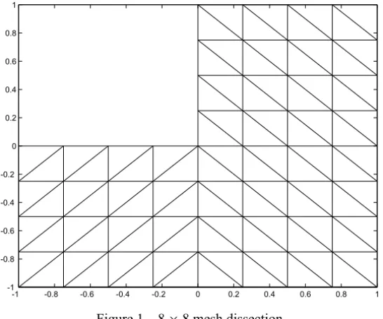
Figure 1 – 8×8 mesh dissection.
we take a finite element subdivision like Figure 1. Information on sparsity of the relevant matrices is given in Table 1. The test problem is set up so that the right hand side function is equal to 1 throughout the domain.
Mesh n m nz(A) nz(B) order ofA
32×32 2240 961 10948 6926 3201
64×64 9088 3969 44932 29198 13057
128×128 36608 16129 182020 119822 52737 256×256 146944 65025 732676 485390 211969
Table 1 – Values ofnandm, nonzeros inAandB, order ofA.
Here we mainly test four preconditioners: R−1, H1, T1 and T. From
Re-mark 2.2, based on the condition number of the matrix, it ensures that the norm of the augmenting term is not too small in comparison with A [35], we set
W−1=20kAk1
kBk2
1
I. One can see [35] for details.
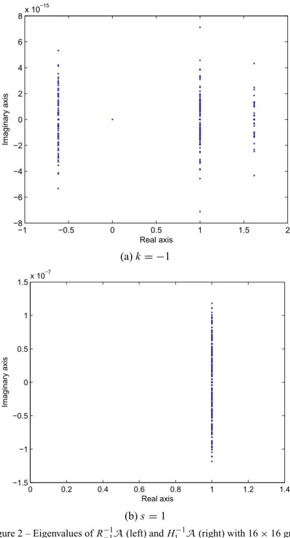
It is well known that the eigenvalue distribution of the preconditioned mat-rix gives important insight in the convergence behavior of the preconditioned Krylov subspace methods. For simplicity, we investigate the eigenvalue distri-bution of the preconditioned matrices R−−11A and H−1
−1 −0.5 0 0.5 1 1.5 2 −8
−6 −4 −2 0 2 4 6 8x 10
−15
Real axis
Ima
g
in
a
ry
a
xi
s
(a)k= −1
0 0.2 0.4 0.6 0.8 1 1.2 1.4 −1.5
−1 −0.5 0 0.5 1 1.5x 10
−7
Real axis
Ima
g
in
a
ry
a
xi
s
(b)s =1
Figure 2 – Eigenvalues of R−−11A(left) andH−1
eigenvalues of the preconditioned matrices R−−11AandH−1
1 Afor 16×16 grid,
where left corresponds to R−−11Aand right corresponds to H−1
1 A. It is easy to
see that the clustering of the eigenvalues ofH1−1Ais more stronger than that of
H1−1Ain Figure 2.
To investigating the performance of the above four preconditioners, in our numerical experiments some Krylov subspace methods with BiCGStab and GMRES(ℓ) are adopted. As is known, there is no general rule to choose the restart parameterℓ (ℓ ≪ n +m). This is mostly a matter of experience. To illustrate the efficiency of our methods, we takeℓ=20. In Tables 2 and 3, we present some results to illustrate the convergence behaviors of BiCGStab and GMRES(20) preconditioned by R−1, H1, T1 andT, respectively. Herei ofT
is equal to 1. Figures 3 and 4 correspond to Tables 2 and 3, which show the iteration numbers and relative residuals of preconditioned BiCGStab and GM-RES(20) employed to solve the saddle point linear systems (1.2), where left in Figures 3-4 corresponds to BiCGStab and right in Figures 3-4 corresponds to GMRES(20). The purpose of these experiments is just to investigate the influ-ence of the eigenvalue distribution on the converginflu-ence behavior of BiCGStab and GMRES(20) iterations. “IT” denotes the number of iteration. “CPU(s)” denotes the time (in seconds) required to solve a problem.
Mesh R−1 H1 T1 T
IT CPU(s) IT CPU(s) IT CPU(s) IT CPU(s)
32×32 5 0.1563 3 0.0938 3 0.1406 5 0.1563
64×64 5 0.8281 3 0.4844 3 0.8281 4 0.6563
128×128 5 4.7188 3 2.7813 3 6.0156 4 3.6250
256×256 5 24.8906 2 10.0625 3 33.4688 4 19.5469 Table 2 – Iteration number and CPU(s) of BiCGStab method.
From Tables 2-3, it is not difficult to see that the exact preconditioners R−1, H1, T1 and T are in relation to the CPU time, and the iteration numbers of the exact preconditioners R−1, H1, T1 andT are insensitive to the changes in
the mesh size by using BiCGStab and GMRES(20) to solve the saddle point linear systems (1.2). Although the exact preconditionersR−1,H1,T1andT are
Mesh R−1 H1 T1 T IT CPU(s) IT CPU(s) IT CPU(s) IT CPU(s)
32×32 3 0.1563 2 0.1250 2 0.1719 3 0.1406
64×64 3 0.8125 2 0.6250 2 1.1094 3 0.7813
128×128 3 4.6719 2 3.7656 2 7.7031 3 4.4844
256×256 3 19.6875 2 14.6563 2 33.0625 3 19.3750 Table 3 – Iteration number and CPU(s) of GMRES(20).
Matrix name order ofA n m nnz(A)
GHSindef/k1san 67759 46954 20805 559774
Table 4 – Characteristics of the test matrix from the UF Sparse Matrix Collection.
number and CPU time. Compared with the preconditioners R−1,T1andT, the
preconditioner H1 may be the ‘best’ choice. Comparing the performance of BiCGStab to the performance of GMRES(20) is not within our stated goals, but having results using more than one Krylov solver allows us to confirm the consistency of convergence behavior for most problems.
Example 2. A matrix from the UF Sparse Matrix Collection [39].
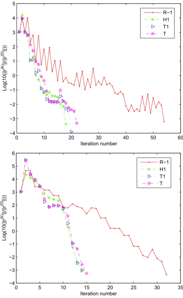
The test matrix is GHSindef/k1san, coming from UF Sparse Matrix Collec-tion, which is an ill-conditioned matrix from Aug. system modelling the un-derground of Strazpod Ralskem mine by MFE. The characteristics of the test matrix are listed in Table 4. The numerical results from using the BiCGStab and GMRES(20) methods preconditioned by the above four preconditioners to solve the corresponding saddle point linear systems are given in Table 5. Figure 5 is in concord with Table 5, where left in Figure 5 corresponds to BiCGStab and right in Figure 5 corresponds to GMRES(20).
From Table 5, it is easy to see that the preconditioners R−1, H1,T1andT are
really efficient when BiCGStab and GMRES(20) methods are used to solve
R−1 H1 T1 T IT CPU(s) IT CPU(s) IT CPU(s) IT CPU(s) BiCGStab 53 96.3594 17 31.5625 19 38.1563 21 50.6406 GMRES(20) 31 61.3906 13 26.2656 13 27.8906 14 39
1 2 3 4 5 6 7 −14
−12 −10 −8 −6 −4 −2 0 2 4
Iteration number
lo
g
(1
0
(|
|r
(k||
/|
|r
(0
)||)))
R−1
H
1
T1
T
(a) 32×32 mesh
1 1.5 2 2.5 3 3.5 4 4.5 5 −12
−10 −8 −6 −4 −2 0 2 4
Iteration number
lo
g
(1
0
(|
|r
(k)
||
/|
|r
(0
)||))
R
−1
H1
T
1
T
(b) 32×32 mesh
Figure 3 (to be continue) – Iteration number of BiCGStab (top) and GMRES(20)
1 2 3 4 5 6 7 −14
−12 −10 −8 −6 −4 −2 0 2 4
Iteration number
lo
g
(1
0
(|
|r
(k)
||
/|
|r
(0
) ||))
R
−1
H1
T
1
T
(c) 64×64 mesh
1 1.5 2 2.5 3 3.5 4 4.5 5 −12
−10 −8 −6 −4 −2 0 2 4
Iteration number
lo
g
(1
0
(|
|r
(k)
||
/|
|r
(0
)||))
R
−1
H1
T
1
T
(d) 64×64 mesh
1 2 3 4 5 6 7 −14
−12 −10 −8 −6 −4 −2 0 2 4
Iteration number
lo
g
(1
0
(|
|r
(k)
||
/|
|r
(0
)||))
R
−1
H
1
T1
T
(e) 128×128 mesh
1 1.5 2 2.5 3 3.5 4 4.5 5 −10
−8 −6 −4 −2 0 2 4
Iteration number
lo
g
(1
0
(|
|r
(k)
||
/|
|r
(0
)||))
R−1
H
1
T1
T
(f) 128×128 mesh
1 2 3 4 5 6 7 −12
−10 −8 −6 −4 −2 0 2 4
Iteration number
L
o
g
(1
0
(|
|r
(k)
||
/|
|r
(0
) ||))
R−1 H1 T1 T
1 1.5 2 2.5 3 3.5 4 4.5 5 −10
−8 −6 −4 −2 0 2 4
Iteration number
L
o
g
(1
0
(|
|r
(k)
||
/(|
|r
(0
) ||))
R−1 H1 T1 T
0 10 20 30 40 50 60 −4
−3 −2 −1 0 1 2 3 4 5
Iteration number
L
o
g
(1
0
(|
|r
(k)
||
/|
|r
(0
) ||))
R−1 H1 T1 T
0 5 10 15 20 25 30 35 −4
−3 −2 −1 0 1 2 3 4 5 6
Iteration number
L
o
g
(1
0
(|
|r
(k)
||
/|
|r
(0
) ||))
R−1 H1 T1 T
the saddle point systems with the coefficient matrix being GHSindef/k1san. It is not difficult to find that the preconditioner H1 are superior to the precon-ditioners R−1, T1 and T from iteration number and CPU time under certain
conditions. That is, the preconditioner H1is quite competitive in terms of con-vergence rate, robustness and efficiency.
5 Conclusion
In this paper, we have proposed three types of block triangular preconditioners for iteratively solving linear systems arising from finite element discretization of the Maxwell equations. The preconditioners have the attractive property to improve the eigenvalue clustering of the coefficient matrix. Furthermore, numerical experiments confirm the effectiveness of our preconditioners.
In fact, in Section 2, our methodology can extend the unsymmetrical case, that is, the (1,2) block and the (2,1) block of the saddle point systems are un-symmetrical.
Acknowledgments. The authors would like to express their great gratitude to the referees and J.M. Martínez for comments and constructive suggestions; there were very valuable for improving the quality of our manuscript.
REFERENCES
[1] Z. Chen, Q. Du and J. Zou, Finite element methods with matching and non-matching meshes for Maxwell equations with discontinuous coeffcients. SIAM J. Numer. Anal.,37(1999), 1542–1570.
[2] J.P. Ciarlet and J. Zou,Fully discrete finite element approaches for time-dependent Maxwell’s equations. Numer. Math.,82(1999), 193–219.
[3] J. Gopalakrishnan, J.E. Pasciak and L.F. Demkowicz, Analysis of a multigrid algorithm for time harmonic Maxwell equations. SIAM J. Numer. Anal., 42 (2004), 90–108.
[4] P. Monk, Finite Element Methods for Maxwell’s Equations. Oxford University Press, New York (2003).
[6] P. Monk, Analysis of a fnite element method for Maxwell’s equations.SIAM J. Numer. Anal.,29(1992), 32–56.
[7] C. Greif and D. Schötzau, Preconditioners for the discretized time-harmonic Maxwell equaitons in mixed form.Numer. Lin. Alg. Appl.,14(2007), 281–297.
[8] C. Greif and D. Schötzau, Preconditioners for saddle point linear systems with highly singular (1,1) blocks.ETNA,22(2006), 114–121.
[9] A. Toselli, Overlapping Schwarz methods for Maxwell’s equations in three di-mensions.Numer. Math.,86(2000), 733–752.
[10] Q. Hu and J. Zou, Substructuring preconditioners for saddle-point problems arising from Maxwell’s equations in three dimensions. Math. Comput.,73(2004), 35–61.
[11] J.C. Nédélec,Mixed finite elements inR3.Numer. Math.,35(1980), 315–341. [12] M. Benzi, G.H. Golub and J. Liesen, Numerical solution of saddle point
prob-lems.Acta Numerica.,14(2005), 1–137.
[13] Y. Saad, Iterative Methods for Sparse Linear Systems. Second edition, SIAM, Philadelphia, PA (2003).
[14] A. Greenbaum, Iterative Methods for Solving Linear Systems. Frontiers in Appl. Math., 17, SIAM, Philadelphia (1997).
[15] M. Benzi and J. Liu, Block preconditioning for saddle point systems with indef-inite (1,1) block. Inter. J. Comput. Math.,84(2007), 1117–1129.
[16] M. Benzi and M.A. Olshanskii,An augmented lagrangian-based approach to the Oseen problem.SIAM J. Sci. Comput.,28(2006), 2095–2113.
[17] T. Rees and C. Greif, A preconditioner for linear systems arising from interior point optimization methods. SIAM J. Sci, Comput.,29(2007), 1992–2007.
[18] G.H. Golub, C. Greif and J.M. Varah, An algebraic analysis of a block diagonal preconditoner for saddle point systems.SIAM J. Matrix Anal. Appl.,27(2006), 779–792.
[19] J.W. Demmel,Applied Numerical Linear Algebra.SIAM, Philadelphia (1997).
[20] S. Cafieri, M. D’Apuzzo, V. De Simone and D. Di Serafino, On the iterative solution of KKT systems in potential reduction software for large-scale quadratic problems.Comput. Optim. Appl.,38(2007), 27–45.
[22] T. Rusten and R. Winther, A preconditioned iterative method for saddle point problems.SIAM J. Matrix Anal. Appl.,13(1992), 887–904.
[23] D. Silvester and A.J. Wathen, Fast iterative solution of stabilized Stokes systems, Part II: Using general block preconditioners. SIAM J. Numer. Anal.,31(1994), 1352–1367.
[24] A.J. Wathen, B. Fischer and D. Silvester, The convergence rate of the minimal residual method for the Stokes problem. Numer. Math.,71(1995), 121–134.
[25] A. Klawonn,An optimal perconditioner for a class of saddle point problems with a penalty term.SIAM J. Sci. Comput.,19(1998), 540–552.
[26] V. Simoncini,Block triangular preconditioners for symmetric saddle-point prob-lems.Appl. Numer. Math.,49(2004), 63–80.
[27] A. Klawonn, Block-triangular preconditioners for saddle point problems with a penalty term.SIAM J. Sci. Comput.,19(1998), 172–184.
[28] P. Krzyzanowski,On block preconditioners for nonsymmetric saddle point prob-lems.SIAM J. Sci. Comput.,23(2001), 157–169.
[29] H.S. Dollar and A.J. Wathen, Approximate factorization constraint precondi-tioners for saddle-point matrices.SIAM J. Sci. Comput.,27(2006), 1555–1572.
[30] H.S. Dollar, Constraint-style preconditioners for regularized saddle point prob-lems.SIAM J. Matrix Anal. Appl.,29(2007), 72–684.
[31] E. De Sturler and J. Liesen, Block-diagonal and constraint preconditioners for nonsymmetric indefinite linear Systems, Part I: Theory. SIAM J. Sci. Comput., 26(2005), 1598–1619.
[32] A. Forsgren, P.E. Gill and J.D. Griffin, Iterative solution of augmented systems arising in interior methods.SIAM J. Optim.,18(2007), 666–690.
[33] C. Keller, N.I.M. Gould and A.J. Wathen, Constraint preconditioning for indefi-nite linear systems.SIAM J. Matrix Anal. Appl.,21(2000), 1300–1317.
[34] V. Simoncini and M. Benzi, Spectral properties of the Hermitian and skew-Hermitian splitting preconditioner for saddle point problems. SIAM J. Matrix Anal. Appl.,26(2004), 377–389.
[35] G.H. Golub and C. Greif, On solving block-structured indefinite linear systems. SIAM J. Sci. Comput.,24(2003), 2076–2092.
[37] S.L. Wu, T.Z. Huang and C.X. Li, Generalized block triangular preconditoner for symmetric saddle point problems.Computing,84(2009), 183–208.
[38] I.C.F. Ipsen, A note on preconditioning nonsymmetric matrices.SIAM J. Matrix Anal. Appl.,23(2001), 1050–1051.