Airfoil Improvement on Horizontal Axis Wind Turbine Suitable for Local Construction in Underdeveloped Countries

(1)

UNIVERSIDADE DA BEIRA INTERIOR

Engenharia

Airfoil Improvement on Horizontal Axis Wind

Turbine Suitable for Local Construction in

Underdeveloped Countries

(Versão corrigida após defesa)

João Carlos Tavares Miguel

Dissertação para obtenção do Grau de Mestre em

Engenharia Aeronáutica

(Ciclo de Estudos Integrado)

Orientador: Prof. Doutor Miguel Ângelo Rodrigues Silvestre Co-orientador: Prof. Doutor João Manuel Milheiro Caldas Paiva Monteiro

(2)

(3)

“First of all, the Big Bang wasn’t very big. Second of all, there was no bang. Third, Big Bang Theory doesn’t tell you what banged, when it banged, how it banged. It just said it did bang. So, the Big Bang Theory in some sense is a total misnomer.” Michio Kaku

(4)

(5)

Acknowledgments

To my parents as they were the ones that allowed for the accomplishment of this dissertation, for my presence in this university and for my personal growth. To my sister that has always supported me, asking me about my academic performance, ready to help me anytime needed.

To my supervisor, Professor Miguel Silvestre for allowing my role in this study, for the readiness and patient given, and mostly for the shared knowledge and hints. To my supervisor, Professor João Monteiro, for the explanations about the Qblade simulations when the results weren’t matching.

To the long date friends, to the academic friends met in this journey, to the Erasmus friends and to the bohemian friends for all the wonderful debates about any random topic.

(6)

(7)

Abstract

This dissertation purpose is to study the impact that a geometry modification of a wind turbine rotor imposes on its performance. The studied wooden rotor, with a diameter of 1.2 m, belongs to a family of small wind turbines that are built by unskilled persons using hand tools with the guidelines of Hugh Piggott. Due to its inaccuracy, the production process delivers a geometry with sharp leading edges. For the performance of an airfoil, the leading edge is one of the most important characteristics to take in mind, and so, the goal of this dissertation was to smooth the airfoils leading edge towards the lower surface in order to widen the 𝐶𝑝− 𝜆 curve of the rotor. To do so, numerical methods were employed to assess such modification on the performance, in a way that the technique could be later applied on the rotor using nothing but hand tools. In a previous investigation, the same rotor here approached in this dissertation, was numerically and experimentally studied for the following windspeeds: 3.0; 3.7; 4.4; 5.5; 7.2 e 7.7 m/s. In the same study, a digital scan was performed on the rotor, one for each blade, resulting in 6 different cross sections each with its chord and incidence angle. The three blades present geometric differences. Having these airfoils characteristics, the QBlade software was used for the design and analysis of the new modified airfoils based on the original Piggott airfoils. The software also allows for rotor design and uses the Blade Element Momentum Theory for the analysis of horizontal axis wind turbines. The performance of both rotors was approximated by averaging the performance of three ideal rotors, each consisting of three identical blades 1,2 and 3. The new airfoils regarding blade 1 and 3, presented better aerodynamic efficiency performance compared to the Piggott airfoils, whereas blade 2 new airfoils did not exhibited any significant improved performance compared to the Piggott airfoils.The dimensionless simulations results from QBlade, portrayed that the averaged rotor with the modified airfoils present better power coefficient (𝐶𝑝) for high values of 𝜆 (ratio between the tangential velocity of the blade tip and the free stream windspeed) when compared to the averaged rotor with the Piggott airfoils. For a constant rotational speed of 500 RPM, the new rotor remarkably withdraws more energy from the flow for low windspeeds. In a hypothetical approach of a optimized turbine production made up by the best modified airfoils, the optimized rotor simulations showed a significant better performance for high values of 𝜆,as well as higher maximum 𝐶𝑝 than the ones from the averaged rotor with the modified airfoils.

Keywords

(8)

(9)

Resumo

O objectivo da presente investigação é estudar a influência que uma modificação na geometria do rotor de uma turbina eólica inflige na sua eficiência. O rotor estudado, de madeira e com um diâmetro de 1,20 m, pertence a um grupo de pequenas turbinas eólicas que são construídas apenas com recurso a ferramentas manuais seguindo as indicações do Hugh Piggott. Este processo de construcção, devido à sua imprecisão, resulta numa geometria que dá origem a um bordo de ataque aguçado. Sendo que o bordo de ataque é um aspecto importante para o desempenho do mesmo, o objectivo desta dissertação passou por suavizar o bordo de ataque do perfil alar a “fugir” para o intradorso, de maneira a ampliar a curva 𝐶𝑝− 𝜆 do rotor. Para tal, recorreu-se a métodos numéricos para avaliar o desempenho de tal modificação, numa perspectiva que esta técnica possa ser aplicada no rotor usando ferramentas manuais, como por exemplo uma lixa. Num estudo prévio, o mesmo rotor que é estudado nesta dissertação foi alvo de um estudo numérico e experimental para as seguintes velocidades de vento: 3.0; 3.7; 4.4; 5.5; 7.2 e 7.7 m/s. No mesmo estudo o rotor foi alvo de uma digitalização na qual, cada pá do rotor foi examinada em 6 secções diferentes e que resultou em 6 perfis alares diferentes com a respectiva corda e o ângulo de incidência, sendo de realçar que as três pás apresentam diferenças geométricas entre si. Tendo estas características, usou-se o software QBlade para o desenho e análise dos novos perfis alares modificados a partir dos originais perfis alares do Piggott. O software permite o desenho de rotores e para a simulação do desempenho de turbinas eólicas de eixo horizontal, o software emprega a Blade Element Momentum Theory. O desempenho real do rotor original e do novo rotor foi estimado a partir da média de três rotores ideais, cada um constituído por três pás idênticas 1, 2 e 3. Os novos perfis alares das pás 1 e 3 revelaram melhor desempenho da sua eficiência aerodinâmica (𝐶𝑙/𝐶𝑑) quando comparados aos perfis oriundos da construção manual do Hugh Piggott, enquanto que os novos perfis da pá 2 não ilustraram qualquer melhoria significativa quando comparados aos perfis originais. Os resultados das simulações adimensionais do QBlade, mostraram que o rotor médio com os novos perfis apresenta melhor coeficiente de potência (𝐶𝑝) para altos valores de 𝜆 (razão entre a velocidade tangencial da ponta da pá e a velocidade do vento) quando comparado ao rotor médio com os perfis do Piggott. Quando submetidos a uma velocidade rotacional constante de 500 RPM, o novo rotor retira notavelmente mais energia do escoamento a baixas velocidades de vento. Numa abordagem hipotética da construcção de uma turbina optimizada composta pelos melhores perfis modificados, as simulações do rotor optimizado ilustraram um significativo melhor desempenho a altos valores de 𝜆 como 𝐶𝑝 máximos mais elevados do que os do rotor médio com os perfis modificados.

Palavras-chave

(10)

(11)

Content

Introduction ... 1 Motivation ... 1 Objective ... 9 Structure ... 9 Literature Review ... 11 2.1 Historical Perspective ... 11 2.1.1 The Windmill ... 11

2.1.2 Wind-powered Generation of Electricity ... 14

2.1.3 Wind Turbine Generators ... 15

2.2 The Wind ... 16

2.2.1. Weibull Distribution ... 17

2.3 Modern Wind Turbines ... 19

2.3.1 Types of Wind Turbines ... 19

2.3.2 Small Wind Turbines ... 21

2.4 HAWT Aerodynamics Basics ... 22

2.4.1 One-dimensional Momentum Theory ... 22

2.4.2 Momentum Theory with Wake Rotation ... 27

2.4.3 Airfoil Terminology ... 31

2.4.4 Blade Element Theory ... 33

(12)

Content

2.5 State of the art ... 42

Methodology ... 47

3.1 The 1200 mm Diameter Hugh Piggott Wind Turbine ... 47

3.2 QBlade Software ... 50

3.2.1 Description ... 50

3.2.2 Airfoil Design and Analysis Module ... 51

3.2.3 Lift and Drag polar extrapolation ... 52

3.2.4 Blade Design and Optimization ... 53

3.2.5 Turbine Definition and Simulation ... 53

3.3 Existing Wind Turbine Airfoil Modification... 53

3.4 BEM Simulations ... 59

3.5 Rotor Power Output ... 66

3.6 General Procedure ... 69

Results and Discussion ... 71

4.1 Methodology Validation Results ... 71

4.2 Airfoils Refinement Effect ... 73

4.3 Modified Airfoils Results ... 74

4.3.1 Blade 1 ... 74

4.3.2 Blade 2 ... 77

4.3.3 Blade 3 ... 79

4.4 BEM simulations ... 82

(13)

Content

4.4.3 Blade 3 ... 86

4.5 Modified Airfoils Rotor Performance ... 88

4.6 Rotor Power Output ... 90

4.7 Optimized Modified Airfoils Rotor Performance ... 94

Contributions ... 99 Bibliography ... 101 Appendix A ... 105 Chapter 1 Annexes ... 105 Chapter 2 Annexes ... 106 Appendix B ... 107 Chapter 4 annexes ... 107

(14)

(15)

List of Figures

Figure 1.1: Change in global mean surface temperature [1]. ... 2

Figure 1.2: Greenhouse gas emissions by economic sector [4]. ... 3

Figure 1.3: Sectoral coverage of international cooperative initiatives [5]. ... 4

Figure 1.4: Renewable energy capacity growth (left) and capacity installed in 2018 (right) [6]. ... 4

Figure 1.5: European Union gross electricity generation by fuel (adapted from [8]). ... 5

Figure 1.6: European Union renewable gross electricity production (adapted from [8]). ... 6

Figure 1.7: Added capacity of onshore and offshore installations in Europe [10]. ... 7

Figure 2.2: Seistan windmill shematic top view [18]. ... 11

Figure 2.1: Seistan Windmill [17]. ... 11

Figure 2.3: Post-Mill design [17]. ... 12

Figure 2.4: European smock mill [17]. ... 13

Figure 2.5: Smeaton’s laboratory windmill rotor testing apparatus [17]. ... 13

Figure 2.6: Brush Windmill in 1888 in Cleveland, Ohio [18]. ... 15

Figure 2.7: Jacob’s turbine [17]... 16

Figure 2.8: Diurnal and nocturnal tertiary circulation [23]. ... 17

Figure 2.9: Weibull probability density function for 𝐴 = 8 m/s [22]. ... 18

Figure 2.10: Weibull probability density function for 𝑘 = 2 [22]. ... 19

Figure 2.11: Different horizontal axis turbine concepts (adapted from [17]). ... 20

Figure 2.12: Different vertical axis turbine concepts (adapted from [17])... 21

Figure 2.13: Flow through a wind turbine represented by a non-rotating disk. ... 23

Figure 2.14: Power coefficient, thrust coefficient and the velocity ratio between the wake and the free stream as a function of the axial induction factor. ... 27

Figure 2.15: Annular stream tube model. ... 28

Figure 2.16: Annular stream tube geometry at the rotor plane. ... 28

Figure 2.17: Axial and angular induction factors as a function of the non-dimensional blade (𝜆 =5). ... 30

(16)

List of Figures

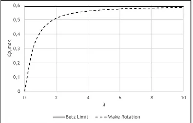
Figure 2.18: Maximum power coefficient obtained with wake rotation as a function of 𝜆. ... 31

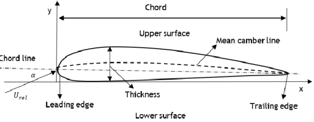
Figure 2.19: Airfoil geometry parameters. ... 32

Figure 2.20: Blade Element schematic model [30]. ... 33

Figure 2.21: Velocity triangle model of the flow incident at a section of the blade. ... 33

Figure 2.22: Blade forces analysis. ... 34

Figure 2.23: Local loads analysis. ... 35

Figure 2.24: Blade pitch angle distribution. ... 37

Figure 2.25: Blade chord distribution. ... 38

Figure 2.26: Tip and Hub Losses [28]. ... 40

Figure 2.27: Circulation distribution along the blade [28]. ... 42

Figure 2.29: Experimental results [15]... 43

Figure 2.28: Stand used to perform the rotor’s calibration [15]. ... 43

Figure 2.30: Average of blade 1, 2 and 3 BEM simulations of WT_Perf and QBlade codes [15]. ... 44

Figure 3.1: Aquila 9.3% smoothed airfoil from the UIUC Airfoil Coordinates Database. ... 47

Figure 3.2: Airfoil scheme within the workpiece [35]. ... 48

Figure 3.3: Tapered shape schematic view [35]. ... 48

Figure 3.4: Schematic view of the twisted windward face [35]. ... 49

Figure 3.5: Workpiece marks to achieve the blade thickness [35]... 49

Figure 3.6: Cross section scheme on how to carve the curved shape [35]. ... 50

Figure 3.7: Software modules inside QBlade [36]. ... 51

Figure 3.8: NACA-63 polar extrapolation to 360º [36]. ... 53

Figure 3.9: Flowchart of the method employed to obtain the smoother airfoil... 54

Figure 3.10: Digital scans of the blades of the rotor [15]. ... 55

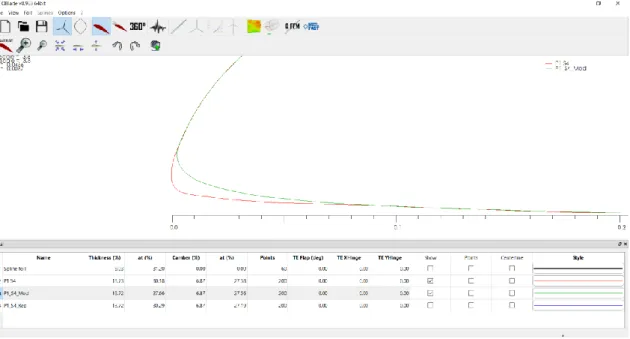
Figure 3.11: QBlade airfoil design module with section 4 (𝑟 = 300 mm) of blade 1 and standard spline foil... 56

(17)

List of Figures

Figure 3.13: XFoil analysis parameters. ... 57

Figure 3.16: Blade 1 section 4 (𝑟 = 300 mm) Piggott and modified airfoil. ... 58

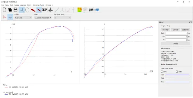
Figure 3.15: Blade 1 section 4 (𝑟 = 300 mm) polar analysis for the Piggott and replicated airfoil. ... 58

Figure 3.17: Aerodynamic efficiency and lift coefficient analysis for the Piggott and modified airfoil of blade 1 section 4 (𝑟 = 300 mm). ... 59

Figure 3.19: Blade 3 Piggott airfoils. ... 60

Figure 3.18: BEM simulation procedure flowchart. ... 60

Figure 3.20: Analysis menu view. ... 61

Figure 3.22: XDirect settings panel. ... 62

Figure 3.21: XFoil analysis parameters. ... 62

Figure 3.23: XFoil analysis for each windspeed of each section of blade 3. ... 62

Figure 3.24: Blade 3 section 1 (𝑟 = 600 mm) 3.0 m/s polar extrapolation. ... 63

Figure 3.25: Re-arranged (green) and non-re-arranged (red) 360º polar. ... 63

Figure 3.26: Blade 3 ideal rotor design with the Piggott airfoils for the 3.0 m/s polars. ... 64

Figure 3.27: 3.0 m/s rotor selection for BEM simulation. ... 64

Figure 3.28: Blade 3 BEM simulation parameters for the 3.0 m/s rotor. ... 65

Figure 3.29: Analysis settings for the BEM Simulation... 65

Figure 3.30: BEM simulations of the ideal rotor consisting of blade 3 Piggott airfoils. ... 66

Figure 3.32: Flowchart comparison between the Piggott and modified windspeed data. ... 67

Figure 3.31: Flowchart of the Excel data management output... 67

Figure 3.33: Flowchart of the wind turbine optimization general procedure. ... 70

Figure 4.1: Averaged blade performance from [15] versus averaged Piggott blade performance from BEM simulations (A: 3.0 m/s; B: 3.7 m/s; C: 4.4 m/s; D: 5.5 m/s; E: 7.2 m/s; F: 7.7 m/s). ... 72

Figure 4.2: Averaged Piggott blade performance with 100 points versus 200 points (A: 3.0 m/s; B: 3.7 m/s; C: 4.4 m/s; D: 5.5 m/s; E: 7.2 m/s; F: 7.7 m/s). ... 73

Figure 4.3: Aerodynamic efficiency and lift coefficient comparison between the Piggott and the modified airfoils of blade 1 (A,B: Section 1; C,D: Section 2; E,F: Section 3). ... 75

Figure 4.4: Aerodynamic efficiency and lift coefficient comparison between the Piggott and the modified airfoils of blade 1 (A,B: Section 4; C,D: Section 5; E,F: Section 6). ... 76

(18)

List of Figures

Figure 4.5: Aerodynamic efficiency and lift coefficient comparison between the Piggott and the modified airfoils of blade 2 (A,B: Section 1; C,D: Section 2; E,F: Section 3). ... 77 Figure 4.6: Aerodynamic efficiency and lift coefficient comparison between the Piggott and the modified airfoils of blade 2 (A,B: Section 4; C,D: Section 5; E,F: Section 6). ... 79 Figure 4.7: Aerodynamic efficiency and lift coefficient comparison between the Piggott and the modified airfoils of blade 3 (A,B: Section 1; C,D: Section 2; E,F: Section 3). ... 80 Figure 4.8: Aerodynamic efficiency and lift coefficient comparison between the Piggott and the modified airfoils of blade 3 (A,B: Section 4; C,D: Section 5; E,F: Section 6). ... 81 Figure 4.9: Piggott and modified rotor power coefficient comparison of blade 1 (A: 3.0 m/s; B: 3.7 m/s; C: 4.4 m/s; D: 5.5 m/s; E: 7.2 m/s; F: 7.7 m/s). ... 83 Figure 4.10: Piggott and modified rotor power coefficient comparison of blade 2(A: 3.0 m/s; B: 3.7 m/s; C: 4.4 m/s; D: 5.5 m/s; E: 7.2 m/s; F: 7.7 m/s). ... 85 Figure 4.11: Piggott and modified rotor power coefficient comparison of blade 3 (A: 3.0 m/s; B: 3.7 m/s; C: 4.4 m/s; D: 5.5 m/s; E: 7.2 m/s; F: 7.7 m/s). ... 87 Figure 4.12: Power coefficient comparison between the average of the 3 Piggott and the 3 modified rotors (A: 3.0 m/s; B: 3.7 m/s; C: 4.4 m/s; D: 5.5 m/s; E: 7.2 m/s; F: 7.7 m/s). ... 89 Figure 4.13: Maximum power coefficient and corresponding optimum 𝜆 of the averaged Piggott and modified rotor. ... 90 Figure 4.14: Averaged Piggott and modified rotor power for the 3.0 m/s windspeed. ... 92 Figure 4.15: Averaged modified rotor power as function of ω. ... 93 Figure 4.16: Averaged Piggott and modified rotor power for a rotational speed of 500 RPM (Y-axis shown with logarithmical scale). ... 94 Figure 4.17: Modified airfoils aerodynamic efficiency and lift coefficient comparison between blade 1, 2 and 3 (A,B: Section 1; C,D: Section 2; E,F: Section 3). ... 95 Figure 4.18: Modified airfoils aerodynamic efficiency and lift coefficient comparison between blade 1, 2 and 3 (A,B: Section 4; C,D: Section 5; E,F: Section 6). ... 96 Figure 4.19: Power coefficient comparison between the averaged of the 3 Piggott rotors and the optimized rotor (A: 3.0 m/s; B: 3.7 m/s; C: 4.4 m/s; D: 5.5 m/s; E: 7.2 m/s; F: 7.7 m/s). ... 97 Figure A.1: Portugal gross electricity generation by fuel (adapted from [8)]. ... 105 Figure A.2: Global employment by RE technology (adapted from [12]). ... 105 Figure B.1: Blade 1 leading edge zoom of the Piggott and the modified airfoil (A: Section 1; B: Section 2; C: Section 3; D: Section 4; E: Section 5; F: Section 6). ... 107 Figure B.2: Blade 2 leading edge zoom of the Piggott and the modified airfoil (A: Section 1; B: Section 2; C: Section 3; D: Section 4; E: Section 5; F: Section 6). ... 108

(19)

List of Figures

Figure B.3: Blade 3 leading edge zoom of the Piggott and the modified airfoil (A: Section 1; B:

Section 2; C: Section 3; D: Section 4; E: Section 5; F: Section 6). ... 108

Figure B.4: Averaged Piggott and modified rotor power for the 3.7 m/s windspeed... 108

(20)

(21)

List of Tables

Table 3.1: Reynolds number according to the windspeed and radial position. ... 61

Table 3.3: Averaged Piggott and modified rotor power for the 3.0 m/s windspeed. ... 68

Table 3.2: Blade radius, windspeed and air density for the 3.0 m/s rotor power. ... 68

Table 4.1: Averaged Piggott and modified rotor power for a rotational speed of 500 RPM. ... 93

Table 4.2: Best airfoil for each blade section. ... 96

Table B.1: Averaged Piggott and modified rotor power for the 3.7 m/s windspeed. ... 108

Table B.3 Averaged Piggott and modified rotor power for the 5.5 m/s windspeed. ... 108

(22)

(23)

Nomenclature

𝐴 Scale factor [𝑚/𝑠]

𝐴𝑑 Rotor area at the disk cross-section [𝑚2]

𝑎 Axial induction factor [−]

𝑎′ Rotational induction factor [−]

𝐵 Number of blades [−]

𝐶𝐷,𝑚𝑎𝑥 Maximum drag coefficient [−]

𝐶𝑝,𝑚𝑎𝑥 Maximum power coefficient [−]

𝐶𝑝 Power coefficient [−]

𝐶𝑁 Normal force coefficient [−]

𝐶𝑇 Tangential force coefficient [−]

𝑐 Blade chord length [𝑚]

𝐷 Drag force [𝑁/𝑚]

𝑑𝑎 Incremental axial induction factor [−]

𝑑𝐶𝑇 Incremental thrust coefficient [−]

𝑑𝑃 Incremental extracted power [𝑊]

𝑑𝐶𝑝 Incremental power coefficient [−]

𝑑𝑄 Incremental torque [𝑁𝑚]

𝑑𝑇 Incremental thrust [𝑁]

𝑑𝑟 Radial thickness at the rotor cross-section [𝑚]

𝐸𝑘 Kinetic energy [𝐽]

𝐸̇𝑘 Kinetic energy flow rate [𝑚3/𝑠]

𝐹 Prandlt correction factor [−]

𝐹ℎ𝑢𝑏 Blade root Prandtl correction factor [−]

𝐹𝑛 Normal force [𝑁]

𝐹𝑡 Tangential force [𝑁]

𝐹𝑡𝑖𝑝 Prandtl correction factor for the blade tip [−]

(24)

Nomenclature

𝑚𝑎𝑖𝑟 Air mass [𝑘𝑔]

𝑚̇𝑎𝑖𝑟 Air mass flow rate through the disk [𝑘𝑔/𝑠]

𝑃𝑎𝑣𝑎𝑖 Available power in the wind [𝑊]

𝑝1 Pressure at cross-section 1 [𝑃𝑎]

𝑝∞ Pressure [𝑃𝑎]

𝑝(𝑈) Weibull probability density function [−]

𝑄 Rotor torque [𝑁𝑚]

𝑅 Maximum rotor radius [𝑚]

𝑅𝑒 Reynolds Number [−]

𝑟 Radial coordinate at the rotor cross-section [𝑚]

𝑟ℎ𝑢𝑏 Hub radius [𝑚]

𝑇 Thrust [𝑁]

𝑇𝑆𝑅 Tip speed ratio [−]

𝑈 Windspeed [𝑚/𝑠]

𝑈1 Windspeed velocity at cross-section 1 [𝑚/𝑠]

𝑈2 Wind velocity at cross-section 2 [𝑚/𝑠]

𝑈𝑑 Wind velocity at disk cross-section [𝑚/𝑠]

(25)

Nomenclature

Greek Alphabet Letters

∆𝑝 Pressure difference between the rotor [𝑃𝑎]

∆𝑝𝑎′ Pressure difference between the rotor with only the effect of the wake rotation

[𝑃𝑎]

Ω Rotor velocity [𝑟𝑎𝑑/𝑠]

𝛼 Angle of attack [°]

𝜃 Pitch angle [°]

𝑘 Shape Factor [−]

𝜆 Tip speed ratio [−]

𝜆𝑟 Local tip speed ratio [−]

𝜇 Dynamic viscosity [𝑁𝑠/𝑚2_]

𝑣 Kinematic viscosity [𝑚2_/𝑠]

𝜌 Volumetric mass density [𝑘𝑔/𝑚3_]

𝜎 Solidity Ratio [−]

𝜙 Relative wind angle [°]

(26)

(27)

List of Acronyms

APREN Asssociação Portuguesa de Energias Renováveis BEM Blade Element Momentum

BET Blade Element Theory

GHG Greenhouse Gas

HAWT Horizontal Axis Wind Turbine

ICI International cooperative initiatives NSA Non-state or subnational actor

RCP Representative Concentration Pathways

RE Renewable Energy

VAWT Vertical Axis Wind Turbine WECS Wind Energy Conversion System

(28)

(29)

Chapter 1. Introduction

Chapter 1

Introduction

Motivation

The natural greenhouse effect is a balanced transfer and transformation energy system on Earth’s atmosphere, terrestrial surface and oceans. This balance means the received energy is equal to the lost energy, making Earth’s climate stay largely stable. Nevertheless, there are factors that cause changes in the climate system. During the last millennium, changes in the Sun energy production, volcanic eruptions and the concentration increase of the greenhouse gases were the main reasons to cause such changes. Water vapor, carbon dioxide, methane and nitrous oxide are greenhouse gases and they are fundamental for our and other living things existence, by trapping some of the sun radiation on the atmosphere, thus making Earth liveable. The most important greenhouse gas (GHG) is water vapor followed by carbon dioxide. Scientists have been observing this disruption in the heat balance since the beginning of the twentieth century, known as global warming. The principal cause of global warming is the increase of greenhouse gases in the atmosphere [1]. They occur naturally but their increase since the beginning of the Industrial Revolution due to anthropogenic emissions (burning of fossil fuel as a source of energy, intensive agriculture and deforestation) have reached levels not seen in three million years ago. Atmospheric carbon dioxide has slowly changed from 260 ppm to 280 ppm during the last 7000 years prior to 1750, while it has increased 40% to 390.5 ppm in 2011. During the same period (1750-2011) atmospheric methane and nitrous oxide have increased 150 % and 20 % correspondingly [2]. As they absorb and emit the sun radiation, their concentration increase means more heat is trapped in the atmosphere, leading to an increase of Earth’s average temperature and, to other effects on Earth’s climate system. These effects are known to be anthropogenic climate changes.

Climate change has a direct impact on human, geophysical, biological and socioeconomic systems. The vulnerability to climate change is how it will damage or harm those systems, and it depends across regions and populations. The resilience to climate change impacts, is the ability of a system to absorb such changes. A developing country is less resilient to the impacts of climate change than a developed one. With these impacts it is fundamental to adapt our behaviour to these changes and mitigate the resulting effects from climate change in the different systems. Climate change affects various human sectors such as agriculture, food, health, water, energy, fisheries, education, nature and ecosystem conservation, among others, in the form of higher temperatures, change in precipitation patterns, snow and ice melting, sea level rise, increase of the frequency and intensity of extreme weather events. The

(30)

frequency increase of extreme weather events has a direct impact on agriculture production, especially severe droughts and extreme high or low temperatures. There is a tendency with temperature increase of the cereal productivity to increase at mid to high latitudes but to decrease at low latitudes. The changes in precipitation will affect the levels of rivers and lakes, limiting access to drinking water, for household use and agriculture use. Forecasts show that there will be a decrease in water availability at mid and low latitudes leading to a water stress for millions of people. The conservation of an ecosystem will be affected with the increase of species risk of extinction and coral bleaching. Also important is how climate change affects human health, and it will have three types of effects: direct effects of extreme climate events; effects caused by environmental damage and tertiary effects caused by the displacement of populations. Some of the potential climate changes scenarios for human health are: increased morbidity and mortality due to heat waves, floods or storms; greater incidence of infectious disease such as cholera, malaria and dengue fever; increased malnutrition, diarrhoea and cardiorespiratory diseases [3].

All these climate changes consequences and impacts are of complex understanding within Earth’s interconnected systems and cycles and therefore, to address such problems is urgent, as the tipping point for humans to hold Earth’s atmospheric temperature change under 1.5 ºC is almost “tipping”, if not already crossed. The Representative Concentration Pathways (RCP) are projection model scenarios used to gather information about future emission and concentration of GHG, aerosols and climate drivers. They are based on a combination of climate models, atmospheric chemistry and global carbon cycle models [1]. In Figure 1.1, the predicted variation of the global temperature from multi-model simulated time series from 1950 to 2100 is different according to each RCP scenario. They concern the approximate total radiative force in year 2100 relative to 1750, as an example, 2.6 𝑊 𝑚2_{for RCP 2.6. The RCP 2.6 represents a} mitigation scenario of very low forcing level, the RCP 4.5 and RCP 6.0 correspond to two stabilization scenarios, and RCP 8.5 is a very high GHG emission scenario. By observing Figure

(31)

1.1, the global temperature is likely to exceed 1.5 °C by the end of the current century relative to 1850 and 1900 for all RCP scenarios except RCP 2.6.

If such point is desired to avoid, the global greenhouse gas emissions must decline drastically. Figure 1.2 portraits the direct GHG emission shares, in % of all total anthropogenic GHG emissions, of five major economic sectors in 2010. The pull-out graphic shows the distribution of indirect carbon dioxide emissions shares from electricity and heat production. “AFOLU” stands for Agriculture, Forestry, and Other Land Use. The industry, AFOLU and energy supply sectors were the major contributors of the GHG emission levels. The total anthropogenic GHG emissions have risen more rapidly from 2000 to 2010 than in the previous three decades, as they have grown 1.0 GtCO2 in 2010 compared to 0.4 GtCO2 in 2000. Also, in these two referred periods, carbon dioxide emissions from fossil combustion and industrial processes were the cause of 78 % of the total GHG emissions [4].

One way to mitigate greenhouse gas emissions, is the use of alternative methods in the energy supply sector. The use of renewable energy in form of wind, solar, biomass, hydric, geothermal and ocean power rather than the conventional use of coal, oil and gas, is a clean and reliable way of GHG emission reduction, a way of reaching a low carbon economy and a path for sustainable development. Within the last decade, a big push was done to promote initiatives for climate change mitigation. The engagement of non-state and subnational actors (NSAs) is a key role in mitigation and adaptation efforts. Their action may come in two categories:

(32)

individual NSA actions and cooperative actions by international cooperative initiatives (ICIs). An ICI is a transnational climate effort of non-state or subnational actors from at least two different countries. ICIs are important in a way that they reduce greenhouse gas emissions, pave the way for the establishment of low-emissions development strategies, ignite technology development and attract more initiatives with their momentum. In the Emissions Gap Report of 2018 from the United Nations Environment Programme, 244 ICIs were registered in the Climate Initiatives Platform, of which 220 are mitigation focused. In 2015, when COP 21 took place in Paris, 44 international cooperatives initiatives were launched, ten more than in 2014. Figure 1.3 shows an overview of the 220 mitigation-focused ICIs for several sectors, where the energy supply sector holds the most ICIs, around 70 % [5].

Recent statistics show that a huge push towards the increase of renewable energy installed capacity over the last decade has being made. Renewable energy can also provide extra benefits such as reducing negative impacts on the environment and health, energy access, be a secure energy supply and contribute to social and economic development in remote and poor rural areas. Renewable energy may be used to generate electricity, for heating and cooling and

(33)

for the transport sector. In 2008, approximately 19 % of global electricity supply originated in renewable energy sources. Between 2008 and 2009, from the 300 GW of new electricity installed capacity, 140 GW concerned renewable sources. Figure 1.4 shows the global evolution of the cumulative capacity of renewable energy for electricity generation over the period of five years, reaching a total renewable energy capacity of 2,351 GW in 2018. The high amount of solar photovoltaics capacity installed goes in accordance to the trend seen in the right graphic of Figure 1.4 by the yellow columns. In 2018 there was an increase of 171 GW in global renewable energy capacity for electricity generation, of which 61 % was installed in Asia. Of the added 171 GW, wind and solar represent 84 %, with 49 GW and 94 GW respectively. Globally, there has been an increase of about 115 GW per year, on average, in non-renewable generation capacity, while renewable generation capacity increased from less than 20 GW in 2001 to around 160 GW or more in 2016, 2017 and 2018. The role of renewables sources in the share of total generation capacity in the world, improved from 22 % in 2001 to 33 % in 2018. In the same period, the global share of renewables in electricity generation capacity have increased from 25 % to 63 % [6].

In the European Union, 227 GW of renewable energy capacity for electricity generation was added between 2009 and 2018, reaching a cumulate capacity of 466 GW. In 2009, the installed capacity of renewable energy for electricity generation in Portugal accounted for 8.9 GW, and in 2018 the cumulative capacity performed up to 13.7 GW [7]. Renewables started to dispute the role of final gross electricity generation major provider in the European Union market, taking the first position in 2014, 2015 and 2016 as observed in Figure 1.5. With the increase of

Figure 1.5: European Union gross electricity generation by fuel (adapted from [8]).

(34)

renewables electricity generation capacity and consequent production, non-renewables have decreased their production, thus leading to less greenhouse gases emissions. Figure 1.6 shows the gross electricity production for every renewable source in the European Union from 1990 to 2016, where it is observed the long reign of hydropower as the major provider of electricity production as well as wind power standing out as the second provider of electricity production since 2006. Although not displayed in Figure 1.6, in 2017, wind power accounted for 362 TWh of the electricity produced, while hydropower only produced 331 TWh, making wind power for the first time the major electricity provider within the European Union renewable mix. With the same trend observed in the European Union, renewables also play a key role in Portugal’s electricity production mix. Portugal’s gross electricity generation chart by fuel is displayed in the attachments, where is observed a clear decrease of electricity generated by Petroleum and Products [8].

According to the Associação Portuguesa de Energias Renováveis - APREN statistics from 2017, Portugal’s electricity production from renewable sources represented 42 % of the total electricity generated. Wind power and hydropower generated 21.6 % and 13.3 % of the total electricity generated respectively, meaning in a total electricity generated of 12.1 TWh and 7.4 TWh.

Globally, the installed capacity of wind power rose from 150 GW in 2009 to 563 GW in 2018. China, with 20 GW, holds the most wind power capacity added in 2018, followed by the United States of America with 7 GW. In Europe and Portugal, there was an increase of 106 GW and 1.8

Figure 1.6: European Union renewable gross electricity production (adapted from [8]).

(35)

Of the current 189 GW of wind power capacity in Europe, 65 % is installed in five countries (Germany, Spain, the UK, France and Italy). Up until recent years most of the wind power installations were onshore. Offshore installations have ascended in recent years as seen in Figure 1.7 by the light blue columns, prompting a considerable growth due to technological advancements such as foundations systems and loosen acoustic regulations. Onshore wind turbine installations in 2018 averaged a power rating of 2.7 MW, while the average capacity of offshore installations was 6.8 MW. The most added capacity was recorded in 2017 with 17,1 GW, with Germany installing a total (onshore and offshore) of 6.5 GW capacity [9]. Of the 10.1 GW added in 2018, 65 % of the installations belong to Germany, the United Kingdom, France and Sweden. Although with less capacity added compared to 2017, Germany installed a total of 3.3 GW of wind power in 2018, currently holding 59.3 GW of cumulative onshore and offshore capacity, followed by Spain with 23.5 GW of only onshore capacity [10].

With all this capacity installed, Europe can cover a reasonable electricity demand with wind as an energy source. For example, in 2018, 14 % of European Union’s electricity demand was generated by wind power with a total wind energy production of 362 TWh, 2 % higher than in 2017. Denmark covered 41 % of its average annual electricity demand with wind in 2018, followed by Ireland and Portugal with a share of 28 % and 24 % respectively. In the previous year, the same countries reported a share of 44.4 %, 24 % and 24.2 % correspondingly. On December the 8th_{, wind energy registered a peak production of 98 GW, supplying one third of}

Europe’s electricity demand [10].

One of the direct socio-economic benefits from the use of renewables, is the gradual drop of a country energy dependence from fossil fuels. As it is logical, renewables will decrease fossil fuels extraction, if such nation has them as natural resources. Otherwise, if a country relies primarily on imported energy fuels, the use of renewables will allow for economic savings in the balance of trade. Taking Portugal as example, the increased use of the renewable generated electricity allowed in 2017, a spare of 770 M € in gas and coal imports, as well as 40

(36)

M € less in carbon dioxide emissions permits. From 2010 to 2017, Portugal saved 6,030 M € in fossil fuel imports and 524 M € in carbon dioxide permits. The specific emissions of the electricity sector in Portugal was of 360 g/kWh in 2017, a reduction in 50 % compared to 1999 when they were at 631 g/kWh [11].

Another driven benefit from renewable energy is employment. In 2017, the global renewable energy industry employed 10.3 million people, representing a growth of 5.3 % compared to the previous year. China alone accounts for 40 % with over 4.1 million jobs. The solar photovoltaic industry has been through a notable growth over the last years with an increase of 8.7 % compared to 2016, leading the employment rate with 3.3 million jobs. A chart of the global RE employment by technology between 2012 and 2017 is displayed in Appendix A. The second industry with most people employed is liquid biofuels with 1.9 million jobs, followed by large hydropower (>10 MW) employing 1.5 million people. Wind power comes in the fourth position employing 1.15 million people across the globe, a decrease of 0.6 % from 2016. China, Germany, the United States of America, India and the United Kingdom represent 76 % of the total jobs in the wind segment. Again, China holds the first place with 44 % of the global wind employment. Europe accounts for 30 % of the wind employment and is a global technology leader especially in the offshore sector. The statistic from 2016 portraits a sector with 344,000 jobs in Europe, representing an increase of 15 % over the previous year [12]. In 2010, there were 41,542 people employed in the Portuguese RE sector, a value that increased to 55,275 jobs in 2017.

All the previous statistics concern large scale wind turbines, grouped into farms which provide power to the electrical grid. By definition, a large-scale wind turbine, although there is no clear and concise establishment, is a wind energy conversion system with a rated capacity of more than 1 MW, or with a rotor diameter superior than 50 m. The current biggest wind turbine belongs to the joint company between Mitsubishi Heavy Industries and Vestas, and it was installed in 2018 in the United Kingdom. The V164-8.8 MW offshore wind turbine that was upgraded from the 8.0 MW version, has a rotor diameter of 164 m and a power rating of 8.8 MW. Nevertheless, the joint company launched during 2018 the V164-10.0 MW offshore wind turbine, and in 2019, the V174-9.5 MW offshore wind turbine with a rotor diameter of 174 m was introduced to the market. One V164.10.0 MW wind turbine can power up to 9,000 UK households. Nevertheless, GE Renewable Energy is another competitor in the offshore industry with the Haliade 150-6MW, a wind turbine with a rotor diameter of 150 m, blades with 73.5 m length, capable of supplying enough electricity for 5,000 European households. The pursuit for better and more efficient wind turbines, has led to the launch of the Haliade-X 12 MW with a 220 m rotor diameter, featuring a 107 m blade and a capacity of 12 MW. Upon its installation, the Haliade-X will become the biggest and most efficient offshore wind turbine, capable of generating clean power to supply 16,000 European households [13] [14].

(37)

Objective

This dissertation purpose is to investigate the hypothetic effect that a shape modification on a wind turbine rotor would enforce on its performance. A graphic user friendly open source software, QBlade, is used to perform the rotor shape modification and to simulate the wind turbine performance. In order to accomplish this objective, intermediate tasks are required such as:

• Performance simulation of the “original” wind turbine;

• Shape modification by smoothing the rotor airfoils leading edge towards the lower surface;

• Performance simulation of the new wind turbine; • Performance comparison and analysis.

Structure

Several chapters compose the lay out of this dissertation.

The first chapter introduces the importance wind power has and will have, to mitigate climate change effects and to ensure a sustainable development for our planet. The dissertation main objective is presented, and the document guidelines are introduced.

Chapter 2 exposes a literature review, starting by exposing a historical evolution of what is nowadays the concept of a wind turbine. The physics behind wind motion is then explained in the second section, followed by a description of modern wind turbines configuration. The aerodynamic theory that QBlade uses for wind turbines performance simulation is settled in the fourth section and the last section exposes what has been scientifically done on the investigation of small horizonal axis wind turbines performance.

The methodology applied in this study is described in the third chapter. In first place, the construction process of the Hugh Piggott wind turbine is shown in order to understand how the rotor is made of three different blades, and secondly, QBlade’s structure and functionalities are presented. After, the process of modifying the airfoils shape and the efficiency simulation of the Piggott and the new rotor is depicted step by step. Another section addresses how both rotors power efficiency was compared, and the last section portrays a flowchart of the general methodology process.

In the fourth chapter, made of 6 sections, the results of the simulations are displayed and discussed. The first section compares the simulation results of the Piggott wind turbine from the work of (Monteiro et al) and from the ones obtained in this study, while the second section

(38)

reflects the effect of the airfoil refinement in the simulations accuracy. The results from the polar analysis of the Piggott and the modified airfoils are illustrated in the third section. As there are geometric differences between blades, the fourth section addresses the simulations performed for each blade assuming an ideal rotor that consists of three equal blades. By averaging the results from the three ideal rotors, an approximate performance for the real rotor is presented. Subchapter 4.6 presents the analysis of both rotors power output for a hypothetic scenario where the wind turbine would work at a constant rotational speed. Chapter’s 4 last section concerns about the best blade airfoil comparison and selection regarding the same blade cross section, and the performance comparison between the averaged results of Subchapter 4.4, and an optimized turbine made with the best modified airfoil of each cross section.

Chapter 5 contains the conclusions withdrawn from the previous chapter and declares whether this dissertation objective was successful or not.

(39)

Chapter 2. Literature Review

Chapter 2

Literature Review

2.1 Historical Perspective

The use of wind as a source of mechanical power for activities such as grinding grain, pumping water or cutting, lasts at least for the past 2000 years. Also, wind was largely used, and it is still used in the present time to power ships using sails. Only in the turning of the nineteenth century due to technological outbreaks, electricity started to be produced from what is nowadays called a wind turbine.

2.1.1 The Windmill

The windmill is a machine that converts the wind’s power into mechanical power. Around the windmill literature, authors agree to accept the Persian windmill as the first historical documented reference of a windmill. The Persian windmill (Figure 2.1), a vertical axis windmill that dates to the tenth century [16], is also known as the Seistan windmill due to the windy conditions of that Persian region (now Eastern Iran [17]), said to reach 45 m/s windspeeds for four months between spring and summer.

Driven by drag forces, the Seistan windmill was inefficient and vulnerable to damage in high winds. Figure 2.2 illustrates how the windmill was enclosed between walls that acted as a convergent to impose the wind towards the sails [19].

In Northwest Europe, the horizontal axis windmill, in which the shaft was placed horizontally, was born in the late twelfth century. Several hundred mills were registered in England by 1086 in the Doomsday Book, but no note was taken on what type they were [19]. Of 23 English

Figure 2.1: Seistan Windmill [17]. Figure 2.2: Seistan windmill shematic top view [18].

(40)

windmills dated before the year 1200, 15 are dated in the 1190’s, five before 1200 and the remaining three in the 1180’s. In the following century, windmills started to become common in Northwest Europe, being a major source of power in the fourteenth century [16].

The European windmill had horizontal axis and was driven by lift forces, being used for mechanical purposes like water pumping, grinding grain, sawing wood or even to power tools. These early mills had four sails, each set at a small angle with respect to the wheel plane of rotation, and were built on posts so that, when the wind changed its direction, they could be turned to face it. This post construction become later known as the Post-Mill design (Figure 2.3). These axes transition reported some engineering problems like the transmission of power from a horizontal rotor shaft to a vertical one; turning the mill into the wind; and stopping the rotor when necessary. Using a cog-and-ring gear mechanism designed by Vitruvius for the horizontal-axis water wheel solved the first problem while the second issue was overcome by rotating the whole system on a central spindle. Stopping the rotor could be solved by facing the rotor out of the wind and applying a frictional braking on the larger gear of the cog-and-ring gear mechanism [16].

The Industrial Revolution marked the turning point for wind and water as a main source of energy, but more drastic for wind. Steam engines powered by coal provided a more compact and powerful source of energy. Coal had the advantage that it could be transported and used when it was needed, as well, in a certain way, did water. In its turning point, the European windmill reached a whole new level of design and technology due to the will of building larger mills. The challenge was to rotate only the upper part (sails, windshaft and brake wheel) of the mill to face the wind instead of rotating the whole body of the windmill. An example of a Tower-Mill design (or smock windmill) can be seen in Figure 2.4. It is necessary to say that there

(41)

or carvings that had little detail. Windmill sails started to get a certain degree and twist. The common sail, mostly developed in Northwest Europe, was given a twist from the root to the tip while the previous sails had a constant angle to the plane of rotation of about 20º [16].

The Industrial Revolution was a time rich in mechanical development that lead to the improvement of the windmill control devices such as mechanically change the sail setting; improve braking and automatically wind the mill. One major development was the invention of the fantail that allow to ease the work of the miller to turn the windmill manually. During the eighteenth century, the windmill started to be scientifically studied and tested. Civil engineer John Smeaton born in England [16], carried out important work that would lead to the basic rules of windmill performance. Using a device that himself mounted and improved from other’s work, Figure 2.5 illustrates his model on a whirling arm. Even in the absence of most of laws of energy, his model allowed him to run tests at constant speeds and taking measures, laying down design and performance principles. Three basic rules that are still important that come from his findings are [17]:

Figure 2.4: European smock mill [17].

Figure 2.5: Smeaton’s laboratory windmill rotor testing apparatus [17].

(42)

• The speed of the blade tip is ideally proportional to the speed of wind; • The maximum torque is proportional to the speed of wind squared; • The maximum power is proportional to the speed of wind cubed.

The windmill use reached its apogee in the seventeenth and eighteenth centuries as new energy sources, that provided power from the combustion of fuel, took place. Although its use may have declined, it continued into the twentieth century supplying isolated populated areas where small amounts of power were required but constant availability was not essential. The typical European windmill in the late nineteenth century, used a 25 m in diameter rotor. In the start of the century, in France there was about 20,000 of these European windmills and in the Netherlands, the industry used wind energy to power 90% of its activity. Still in the early twentieth century, Germany had more than 18,000 windmills and 11 % of the Dutch industry was based on wind energy [20].

With no association to the milling of grain, the term wind turbine is nowadays established as the machine capable of harnessing the wind energy for different applications together with several other devices that complete a power plant, such as mechanical transmission, nacelle, tower and control gear [16].

2.1.2 Wind-powered Generation of Electricity

The high cost of running transmission and distribution lines from central stations to dispersed habitations and the first appearances of small electrical generators at the end of the nineteenth century would encourage people to use wind for electricity generation. In the United States of America, Charles F. Brush, inventor, builder and industrialist in the electrical field, erected in 1888 a pioneer windmill-generator named the Brush windmill (Figure 2.6). Being the first windmill to generate electricity it had a post mill configuration, and the rotor with 144 blades was 17 m in diameter on a tower 18 m high. The rotor was a solid-wheel type, with a tail vane area of 112 square meters. It ran for 20 years until 1908 supplying 12 Kw of DC power for charging batteries mostly for 350 incandescent lights. Charles’ windmill was a landmark in the multivane type. It was one among the largest built; it introduced the high step-up ratio (50:1) to windmill transmissions, assured by two belt-and-pulley sets in tandem to produce a full load dynamo of 500 rpm; and it was the first to mix structural and aerodynamic windmill features with the recent electrical technology [16].

In 1891, Danish professor and scientist Poul LaCour [19] was chosen to accomplish scientific research at the windmill experimental station established by the Danish State at Askov. LaCour was one of the most important pioneers in the transition from windmills to wind turbines. Introducing principles of the new science of aerodynamics, LaCour research purpose was to

(43)

was one the first persons in the world to use a wind tunnel. The LaCour turbine rotor was composed by plane and rectangular blades with a swept area of up to 23 m in diameter supported on steel framework towers with 23 m high [19]. One notable feature, was that LaCour used energy produced from the wind to electrolyse water, resulting in hydrogen that was burnt to illuminate his laboratory. Around 1910, villages around Denmark were electrically powered by these machines, equipped with 100 to 300 Ampere-hour capacity storage batteries. During windless periods these machines could meet demands up to 10 days.

2.1.3 Wind Turbine Generators

Until World War II, wind-generated electricity was mostly used to generate DC current to charge batteries. The development of the aeronautical science in the early twentieth century inspired the application of the propeller studies to the wind turbine. This led to the initial use of aerodynamic profiles and improvement in the power coefficient [19]. In the United States of America, small wind turbine generators become widespread after the Brush windmill. Being mostly pioneered by Marcellus and Joseph Jacobs, which they started to develop in 1925, their three-bladed rotors had high performance, minimal maintenance and good structural integrity (Figure 2.7). A 32-V DC model could produce 2,500 W and a 110-V DC generator delivered up to 3,000 W [16]. Jacobs rotor most notable feature was the passive pitch control system where the blades feathered with increasing rotor speed.

The early 1930’s saw the introduction of an innovative vertical axis wind turbine patented by French engineer Darrieus, having two or three curved blades attached top and bottom to a central shaft. Darrieus also designed a two-bladed horizontal axis turbine with 20 m in diameter with a maximum power coefficient of 0.347 [19]. In the same decade the wind turbine configuration had settled down having a horizontal axis three bladed rotor upwind of the tower, working at variable speed with its blades at a fixed pitch angle. Even though these machines, generating low-voltage direct current, were reliable and with little maintenance, they did not

Figure 2.6: Brush Windmill in 1888 in Cleveland, Ohio [18].

(44)

have the chance to stand against central stations power as a source of electrical energy. After World War II, along with the first concerns that fossil fuels reserves were finite, with fuel shortages and an increasing knowledge of aerodynamics, the development of larger wind power plants was getting more attention. However, some large-scale wind turbines had been already constructed prior to World War II. The Union of Soviet Socialists Republics took the first step by constructing a 100-kW 30 m diameter wind turbine in 1931 at Yalta on the Black Sea [19]. Being a three bladed rotor, it outputted a maximum coefficient power of 0.162 and it was the first wind powered system to be connected to an existing grid.

Other major achievement of the early large-scale wind turbine is credited to American engineer Palmer C. Putnam that stated that large wind turbines should supplement central power plants. In 1934 he got the S. Morgan Smith Company of York, Pennsylvania (known for manufacturing hydraulic turbines and electrical equipment) to fund its megawatt wind turbine generator prototype [19]. On October 10, 1941, the two bladed rotor, 53.3 m in diameter and with the synchronous generator, delivered electricity to the network for the first time [16].

To close this section about wind turbine generators, one final note is made to the implemention of an electric motor to turn the rotor into the wind by Danish F.L Smidth Company [19]. Developed by Johannes Juul after World War II, the Gedser turbine as it is known due to the location where it was installed, used an induction generator and aerodynamic stall for power control [17]. Between 1956 and 1967 it generated about 2.2 million kWh [21].

2.2 The Wind

Wind is air in motion relative to Earth’s surface. Ultimately, the Sun is responsible for air motion by the pressure differences created by the uneven heating of the Earth surface, with more

(45)

pressure and density, setting up convective forces in the lower layer (troposphere). This result, globally, in hot air to rise at the tropics and flow to the poles. Locally, heated air rises creating depressions [22].

Another important factor in the air movement is the Earth’s rotation, resulting in two aspects. One of them, the Coriolis force that act upon an air particle, accelerates it to the right of its direction of motion in the Northern hemisphere and to the left in the Southern hemisphere. The other effect accounts that an air particle has an angular momentum from the west to east, and as it moves closer to the poles (but remaining at the same altitude) it reaches the axis of rotation, where according to the conversation of angular momentum the velocity of the air particle increases [21]. This second effect is more apparent at middle latitudes and originates the Westerlies winds which are the ones better suited to extract energy This explanation is a general one for a spherical model surface and accounts as a large-scale atmospheric circulation. Local effects must be taken in account such as orography, roughness or the fact that landmasses heat and cool faster than water masses. Hurricanes, monsoons or cyclones constitute the secondary circulation scale, while an example of tertiary circulation is land and sea breezes, valley and mountain winds, or thunderstorms or tornadoes [23]. In Figure 2.8, an example of tertiary circulation is visible, where during the day, the air in the top gets warmer and rises creating a pressure difference due to the cold air in the valley. Hence the air moves towards the top and at night the opposite happens.

2.2.1. Weibull Distribution

Before even wind turbines can be designed, a complex siting process most occur to evaluate where to install the wind turbine or the wind farm in order to maximize the performance while reducing parameters such as noise, environmental and visual impacts, and overall cost of energy. Thus, estimating the wind resource of a certain location is one of the many fundamental aspects to take in account. In the final wind assessment evaluation, the desire is to have a detailed spatial variability of the wind resource across the studied location and the temporal variation over longer time scales. Some of the methods used to determine the wind resource at a certain location are ecological methods, the use of wind atlas data, computer modelling, mesoscale weather modelling, statistical methods and long-term site specific data collection [24].

(46)

Frequency distribution of wind speed and persistence are two parameters commonly used to characterize the wind resource of a certain site. Persistence gives the statistics on the continuous time the wind maintains a certain speed, while the frequency shows the cumulative time the wind blows at a given value. They are important factors for wind turbine design and siting as the frequency distribution allows to calculate the energy input of the wind turbine and persistence the assessment of the wind energy potential [20]. To assess this frequency distribution, several non-Gaussian distributions were suggested being the Weibull distribution the one that ended having the most use for wind load and energy assessment studies. The Weibull probability density function is given by:

𝑝(𝑈) = (𝑘 𝐴) ( 𝑈 𝐴) −1 𝑒𝑥𝑝 [− (𝑈 𝐴) 𝑘 ] (2.1)

Where 𝑘 is the shape factor, 𝐴 the scale factor (m/s) and 𝑈 the free stream wind speed (m/s).

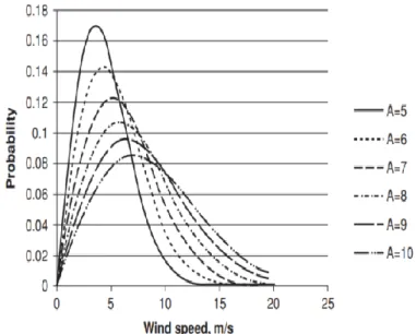
In Figure 2.9, it is visible the sharpening of the curve with the increase of the shape factor meaning there will be less wind variation and higher wind speeds will be less probable. Also, the increase of the shape factor tends to turn the curve into a Gaussian distribution for shape factors over 3. On the other hand, Figure 2.10 illustrates that the increase of the scale factor will extend the curve over the X-axis meaning the higher probability of occurring higher wind speeds at a hypothetical location.

To summarize, it is important to notice that with wind speeds measurements throughout a year, it is possible to view that strong winds are rare while moderate winds are more common. The mean wind speed or the scale factor say how windy in average the location is, while the shape

(47)

2.3 Modern Wind Turbines

The current term wind turbine is shortened from wind turbine generator, name given if the wind machine final purpose is the production of electricity through a generator rotated by the force wind imposes upon the rotor. To give a brief sight about the principle used by any wind turbine it is necessary to refer to the typical aircraft propeller as a rotary mechanism shaped by airfoils that imposes energy (from an external source) into the fluid producing a thrust force in the sense of the movement [25]. However, the wind turbine does the reverse, where it extracts the available power in the fluid stream producing a drag force in the sense of the flow. Withdrawing the scientific words, the goal of a propeller is to push the air through, while wind turbines seize the air displacement. Any wind conversion energy system can be divided according to if they are driven aerodynamically by lift or drag.

2.3.1 Types of Wind Turbines

As said above, wind turbines are defined as lift or drag driven. These two terms will be further explained in detail. Also, during the historical perspective, the horizontal and vertical axis terms were introduced. Although the reference to the wind turbine development in Subchapter 2.1 stagnated little after World War II, the concept of the wind turbine to supply electricity evolved to what it is known nowadays as several wind turbines making up a wind farm for electricity production and distribution to the network. Prior to World War II little development took place mostly in western Europe. It was only when the 1970’ oil crisis struck that the interest in wind energy rose, with a lot of efforts taken by the United States of America, Germany, Denmark and Sweden [21]. By the end of the twentieth century, the largest US wind turbine manufacturer Kennetch Windpower, moved to Europe where, with the apprehension of

(48)

nuclear power and the ever-common effects of global warming being felt, an even stronger push for wind energy took place [17].

Nowadays, the most common type of wind turbine for commercial applications is the horizontal axis wind turbine, also known as HAWT and referred as “propeller-type” due to the basic principles of an aircraft propeller that are applied to HAWT rotors. Generally, a wind energy conversion system is composed of some subsystems such as the rotor, the power train, the nacelle, the tower structure, the foundation, power control and the ground equipment station. Horizontal and vertical-axis turbines share most of these subsystems and components, but some of the configurations are different. For example, a VAWT does not need a yaw mechanism as it accepts winds from any direction. To summarize, wind turbines can be classified according to its design (vertical or horizontal) and according to its size or power rating. Horizontal axis wind turbines with rotors less than 12 m in diameter are classified being small scale; from 12 m to 45 m they are medium scale and over 46 m they are large scale. For power rating, small-scale wind turbine are the ones with less than 40 kW; between 40 kW and 1 MW they are classified as medium-scale and large-scale for more than 1 MW [26]. Throughout the second half of the twentieth century different concepts of wind turbines beyond the traditional HAWT and VAWT were designed and built. None of them will be explained in detail but Figures 2.11 and 2.12 summarize most of the concepts invented.

(49)

2.3.2 Small Wind Turbines

As the wind turbine that is studied in this work is of a small-scale, it is logical to present a general overview on the small-scale wind turbine systems. During the 1970’s, a big push by the United States of America government was made as little performance or engineering data was available for the small-scale application. Analytical and experimental projects were performed under the Federal Wind Energy Program that gave results for later development and assessment of small-scale turbines [27]. In a typical small-scale HAWT, the rotor, tower and power train are the fundamental subsystems. Most commercial small wind turbines are horizontal axis, have an upwind configuration and have passive controlled systems for speed and power regulation. Upwind or downwind refers to the location of the rotor with respect to the tower. Some small wind turbines have fixed pitch blades, as variable pitch mechanisms are costly and require periodic maintenance, relying then on aerodynamic stall to limit peak power. As mentioned before, Jacob’s turbine used a fly-ball governor activated by centrifugal forces to mechanically change the pitch of its blades. A model employed and patented by Bergey Windpower Company

(50)

[26], used weights at the blade tips to twist them to their optimum position, though it did not limited power but helped to start the rotor rotate in low winds.

Whereas in larger-scale wind turbines, yaw control is done by rotating the nacelle to face the rotor to the wind with the use of an electric motor, in a small-scale this is done by weather-vaning. The turbine turns on a bearing by the action of wind forces upon the tail vane. Referring to this mechanism is implicit to note the furling mechanism, that protects the rotor from extreme high speeds and prevent the generator from overheating if not stopped. At high wind speeds vertical furling will tilt the rotor upwards and horizontal furling faces the rotor towards the tail vane. The axial force that acts on the rotor (thrust) causes a yawing moment which thanks to a leverage turns the rotor out of the wind.

Small turbines have generally three blades due to higher dynamic stability than one or two bladed rotors. Blades are often made of wood or wood-epoxy laminates that can be carved or molded but some concepts were made with cloth, fiberglass or laminates. As small turbines operate at different windspeeds it is important to control the rotor in high winds in order to waste the excess power. Mechanical brakes applied to the generator drive shaft are often the usual solution. Another form to control the rotor for small scale wind turbines are blade tip devices, where the outer section of the blade is turned, making the rotor to stop by aerodynamic drag or reducing its speed. There are three types of tip devices which are tip brakes, buckets and pitchable tips [26].

Tower configuration for small wind turbines tend to have a higher height to rotor diameter ratio in order to place the rotor to catch more energetic wind and to get above near obstacles. Some configurations are: shell, stepped shell, lattice or guyed shell. Tower materials for small scale wind turbine range from wood, fiberglass, concrete or tubular steel.

As small wind turbines operate with higher rotor speed than the counterpart large commercial wind turbines, the tradeoff of the transmission-generation system is different. The power train subsystem in general consists of a turbine shaft, a gearbox, a generator drive shaft, a rotor brake and an electrical generator. Most small turbine are direct-driven to the rotor with permanent magnet generators, with no gearbox, turbine shaft or generator drive shaft, but this design does require a converter to obtain a constant frequency [21].