Numerical Analysis into the Effects of the
Unsteady Flow in an Automotive Hydrodynamic
Torque Converter
Pablo De la Fuente, Horst Stoff, Werner Volgmann and Marek Wozniak
Abstract—In this paper the characteristics of a three dimen-sional, incompressible, turbulent, unsteady flow within a one-stage two-phase automotive hydrodynamic torque converter was numerically simulated and analyzed. For the investigation the finite volume method has been employed.
The commercial 3D Navier-Stokes Software CFX of ANSYS Inc. was used to investigate the flow inside a torque converter. The software solves the incompressible Reynolds-Averaged-Navier-Stokes (RANS) equations on the entire flow domain using thek-ǫturbulence model. To compare the simulation with experimental results, the nondimensional characteristics were used. The flow field is determined by the blade position of both rotors, which have different rotating velocities. Discrepancies between the steady and unsteady simulations were found and discussed. The unsteady flow at the pump exit and turbine inlet will be analized through instantaneous flow fields in a period.
Index Terms—hydrodynamic torque converter, CFD, un-steady flow, fluid flow simulation.
I. INTRODUCTION
T
HE fluid in a hydrodynamic torque converter (H.T.C.) is responsable for the torque conversion and power transfer from the engine to the transmission and influences the propulsion efficiency. H.T.C. are commonly used in vehicle power transmission systems such as cars, buses and locomotives. Its typical configuration consists of a pump, driven by the engine that transmits the generated angu-lar momentum, a turbine that transmits the torque to the transmission and a stator, which makes possible the torque conversion through the redirection of the flow to the pump. Some advantages are the capacity to provide torque am-plification during the start-up conditions, a soft start from standstill and the capacity for damping transmission through the absorbtion of torsional vibrations introduced from the engine. One disadvantage is the higher fuel consumption and lower efficiency compared with the gear transmission. So it is necessary to optimize its operating work through understanding the flow behaviour. The internal flow within H.T.C. is three-dimensional, turbulent, viscous, complex, highly unsteady and difficult to analize because of the operating conditions that consist of three elements rotating at different velocities.The two principal unsteady problems concern the ex-ternally forced unsteadiness like the blade-row interaction,
Manuscript received March 04, 2011; revised March 28, 2011. This work was supported by DAAD (Deutscher Akademischer Austauschdienst).
P. D., H. S. and W. V. are with the Department of Fluid-Energy Machines, Ruhr-University Bochum, Germany (email: [email protected], [email protected], [email protected]).
M. W. ist with the Technical University of Lodz, Poland (email: [email protected]).
where the geometry of the flow changes with the rotation of the row and the self-excited unsteadiness like the turbulent motion. Due to the proximity of the components there is a mutual interaction that causes periodically unsteady forces, which are caused due to blade/wake interaction, potential flow interaction and 3D flow effects. Most turbomachinery flows are inherently und strongly unsteady in nature. In many cases a steady flow is assumed for convenience. However, when it becomes necessary to invoke more realistic unsteady analysis this assumption shows disadvantages.
Unsteady flow phanomena like blade row interaction should be investigated through truely unsteady calculation [1]. In addition, the transition between rotating and sta-tionary motion can cause unsteady loading on the blades. The complexity of the flow field is directly influenced by geometric considerations like the spacing between blades. In the last years CFD tools make possible to reduce the cost and save time for the flow analysis and have been used to predict the flow in turbomachinery because of its property to deliver fast predictions of instantaneous flow field states by numerical calculation. CFD tools use the computer resources to calculate the flow by complex mathematical models.
In a number of papers the performance of H.T.C. have been studied with CFD tools [2]–[4] and have been demonstrated how complex the flow is inside the machine. Measurements have been discussed in [5], [6]. Schulz [4] used a finite volume method in calculating three-dimensional, incom-pressible, turbulent flow. Steady and unsteady calculations to simulate the pump/turbine interactions were performed. Their calculations showed that unsteady rotor-stator interaction was negligible, but needed to be accounted for the unsteady interaction between the pump and the turbine. They came to the conclusion that viscous effects were not fully reproduced. Roecken [7] investigated the flow in a H.T.C. and unsteady pressure curves were measured between the two rotors and were compared with calculations obtained from a finite volume procedure. The comparison of torques showed a good agreement so that the authors came to the conclusion that experimental analysis could be described by numerical calculations.
The H.T.C. used in this paper was designed byZF Sachs AG and its geometry was published in [8]. The one-stage two-phase W240 H.T.C. has an outer diameter of 240[mm]. The pump contains Zp =31, turbine Zt =29 and stator Zs=11 blades respectively. The operating fluid is Automatic
Transmission FluidATF LT 71141whose densitiy isρ=802
[ kg/m3
] and the viscosity is ν =0,00653 [ Pa s] at 95
It is recognised that Navier-Stokes simulations can provide useful information to understand of unsteady effects in turbo-machinery [10]. In H.T.C. the unsteady flow is governed by the RANS Reynolds-Averaged-Navier-Stokes transient equa-tions for an incompressible flow by the turbulent viscosity hypothesis. The calculations were all done with the standard
k−ǫturbulence model [11]. The continuity and momentum equations for an incompressible flow are respectively:
∂Uj ∂xj
= 0 (1)
∂Ui ∂t +Uj
∂Ui ∂xj
=−1 ρ
∂P ∂xi
+ ∂
∂xj
ν
∂U
i ∂xj
+∂Uj
∂xi
−ui′uj′
−ρ(2ǫijkωjuk+ωiωjxj−ωjωjxi) (2)
Wheret is the time, U(u, v, w) the velocity vector of the flow, P the pressure, ρ the density and ν the kinematic viscosity of the fluid. In the eddy-viscosity turbulence model the Reynolds stresses ui′uj′ are assumed to be proportional
to the mean velocity gradients with the constant turbulent viscosity. These equations are time-averaged over a period T. The values of the turbulent kinetic energykand turbulent energy dissipationǫ are obtained by solution of the conser-vation equations (3) and (4):
∂k ∂t +Uj
∂k ∂xj
= ∂
∂xj
ν+ νt
σk
∂k
∂xj
+Pk−ǫ (3) ∂ǫ
∂t +Uj ∂ǫ ∂xj
= ∂
∂xj
ν+νt
σǫ
∂ǫ
∂xj
+c1ǫ ǫ
kPk−c2ǫ ǫ2
k
(4) Wherec1ǫ,c2ǫ,σǫandσk are constants.Pkis the turbulence
production due to viscous forces. To obtain a numerical solution these partial differential equations must be first discretised on a grid that covers the flow domain.
III. SIMULATION OF THEINTERNALFLOW It will be assumed that the flow is three-dimensional, incompressible, viscous and turbulent. The pump speed stays constant nP = 2000 min−
1
and the turbine speed changes depending on the speed ratio. The Reynolds number is
Re = ωP·d2P, external
ν = 1481802[−]. At the interfaces a frozen
rotor and a transient rotor-stator model were used for a steady and unsteady simulation respectively. The advection terms of the flow will be solved with the advection scheme option High Resolution with Second Order Differencing. The H.T.C. works like a closed circuit because the working fluid is not subjected to external forces except the forces applied by the components. By the calculation the flow will adjust itself by a closed loop algorithm depending on the boundary conditions at inlet and outlet according to the speed ratioν. A converged steady simulation with blades at standstill was used as initial value for the unsteady case. For the unsteady simulation a time step ∆t is needed, in which the relative position of the rotors will be updated. The unsteady simulation was performed for six different operating points between 0.01 and 0.8, which are characterized by the speed ratio (ν = nt
np).
For the unsteady simulation at design point ν=0.7, which corresponds to the highest value of the efficiency, the time step was calculated by using (5). This time step size has been
Fig. 1. Three-dimensional Computational Analysis Model
Fig. 2. Computational Mesh at Center Planes (Mid Section) Turbine (right)- Stator (center) - Pump (right)
chosen in order to resolve the unsteadiness in the pump-turbine interaction area with 33 time steps. This time step coincides with the Courant Number 4.6.
∆t= 1 (ωp−ωt)·
1
Zp·
1
33 = 9.75·10
−5
[s] (5) One complete turn of the pump coincides with 309 ∆t. At ν=0.7 after 900 time steps and the reach of three same periods the results were considered periodic. The time of the steady computation was approximately 597 minutes. By the unsteady calculation the time necessary to reach three same periods was about 6000 minutes (700∆t) with 7 loops for every time step. The calculations have been made on an Intel Core i3 using four processors in parallel. Starting from a converged steady-state solution, a converged unsteady solution can be obtained in a matter of five days. As conclusion, an unsteady simulation consumes ten times more CPU time compared to the steady method.
A. Calculating mesh
The flow will be discretized in a finite volume mesh to carry out the numerical simulations. The virtual model of the H.T.C. involves the geometry and the circulating three-dimensional flow. The development of the CAD Model, shown in the Fig. 1 and the study of the quality of the mesh were presented and developed in the previous work [12], [13]. The mesh convergence study showed that beyond 400000 points the results are almost the same proving the grid independence of the solution. The mesh was created for one passage of each element (P1T1L1) and copied for the comparison model (P3T3L1), which contains 3 pump, 3 turbine pitches and 1 stator pitch. With the periodicity option and repeated boundary conditions the full H.T.C. was modelled in order to reduce time and computer memory.
Fig. 3. Numerical Grid of the P3T3L1 Model
TABLE I
OVERLAPPINGRELATION AT THEINTERFACES
Pitch ratio W240(P1T1L1) W240(P3T3L1)
P/T 0,935 0,935
T/L 0,379 1,138
L/P 2,818 0,939
of the model P1T1L1. The total number of elements of the P3T3L1 model is 1189737 elements. Both models are identical in each pitch computational grid but different in the number of computed pitches used in each component. For an optimum analysis the net pitch change across the interfaces must be close to unity [14]. The table I shows the pitch ratio values, which correspond to the fractional change areas of the two connected components.
The table I shows clearly that the model P3T3L1 results in a pitch ratio close to the ideal value. The results and compar-ison of both models through their characteristic lines will be presented in the next step, where the torque conversion and the torque coefficient will be compared with measurements.
B. Performance characteristics
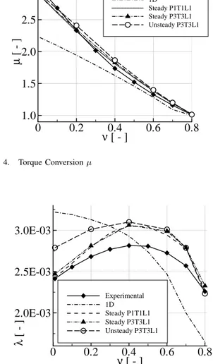
In this chapter the calculated performances of the H.T.C. will be compared with measurements. For this purpose, the torques will be calculated for validation. The non-dimensional characteristics of the H.T.C. consist of two curves determining torque conversion µ and torque coeffi-cientλas a function of rotational frequencies (ωP,ωT) and
torque (MP,MT) of the pump and turbine:
ν = nt
np
; µ=
MT
MP
; λ= MP
ρ·ω2
P·d
5
P,external (6)
To cover one blade pitch of the pump and turbine the period was calculated byν=0.7. The period of the pump and turbine are TP=10∆t and TT=15∆t respectively. Then the
period of the unsteady solution is 60∆t, which corresponds to the time after which the pump and turbine blades are in the same relative position again. After performing the steady and unsteady analysis of the H.T.C. the evaluation of the quality of the CFD simulation will be studied by comparing the numerical and experimental characteristics [8] concerningλ
andµ at speed ratios 0.01-0.8. To obtain the time-averaged torque for the unsteady condition at each operating point the data of one period are averaged. The 1D calculations have been made with the fluid friction factors 0.2 and shock loss coefficient 1.0 for the losses. The efficiency will not be plotted because it provides no new information (η=µ·ν).
To obtain the torque on each component, the force on the blade surface was integrated, so that with the radius to the rotating X-axis the torque can be calculated. The comparison
ν
[ - ]
µ
[
-]
0
0.2
0.4
0.6
0.8
1.0
1.5
2.0
2.5
3.0
Experimental1D Steady P1T1L1 Steady P3T3L1 Unsteady P3T3L1
Fig. 4. Torque Conversionµ
ν
[ - ]
λ
[
-]
0
0.2
0.4
0.6
0.8
2.0E-03
2.5E-03
3.0E-03
Experimental 1D
Steady P1T1L1 Steady P3T3L1 Unsteady P3T3L1
Fig. 5. Torque Coefficientλ
is showed in the Figs. 4 and 5. The torque coefficient has a slightly larger discrepance than the torque conversion results. However, the torque conversion and the torque coefficient are in accordance well with experimental data. Concerning
µ, the torque calculations demonstrate that the time-average torques given by the unsteady calculation are higher and have a better agreement with the measurements than those from the steady calculation (µ). As it can be seen the presented calculated three-dimensional characteristics are representing the behaviour of the experimental results. As far as λ is concerned, the results from the steady simulation show a better agreement with the experimental data. Despite the deviation of the pitch ratio of the P1T1L1 model from the ideal value, however this agree with the measurement as well as the P3T3L1 model. The data show explicitly that the increase ofλis due to the unsteady flow. At small operating points theλdeviation increases because the unsteady pump torques are higher. This confirms the trend in the simulation and will be used to study the internal flow effects in the H.T.C..
Timestep
0
500
1000
10
-610
-510
-410
-310
-210
-110
010
1MAX P-Mass MAX U-Mom MAX V-Mom MAX W-Mom
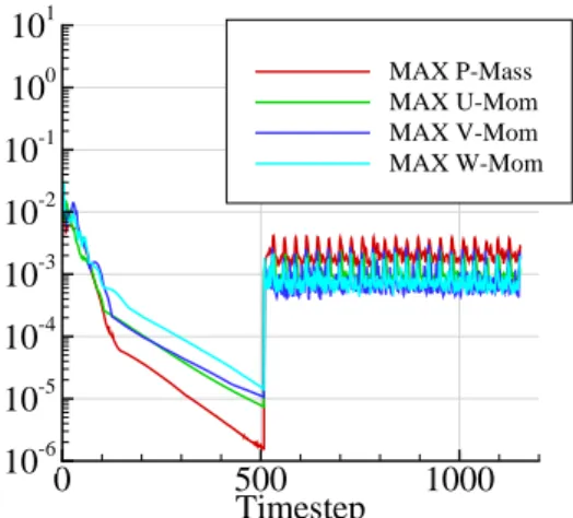
Fig. 6. Convergence History at Design Pointν=0.7
TABLE II
STEADY ANDTIME-AVERAGEDUNSTEADYTORQUES ATν=0.7
Method MP[N m] MT[N m] µ Steady 78.18 93.10 1.1908 Unsteady 78.21 93.36 1.1937
Experimental – – 1.16
periodic flow behaviour. For example at ν=0.8 about 500 iterations were needed for the convergence of the steady simulation and 400 iterations were required to etablish three same periods (T = 40∆t) under the maximum residual below
10−3
. The table II shows that the calculated torques atν=0.7 have very small differences and the torque conversion µ
agree well with the experimental value. We can see that the unsteady µ is only 2.9% higher than the experimental data and the steady µ about 2.7%. The differences between the global valueµin both calculations are very small.
The Fig. 7 shows the oscillation of the torques at ν=0.7. The steady simulation does not account for transient effects such as acceleration or inertia, because of that the steady simulation is not able to resolve the torque oscillations as shown by the plot. The time-averaged unsteady torques are higher than the steady torques because of the unsteady flow. This can result due to the unsteadiness depending on the relative position of the blade that causes the torque oscillation. The blade motion is sustained by extraction of energy from the uniform flow during each blade passage with the corresponding frequency.
It should be noted that these torque fluctuations are the oscillation from the time-averaged values used for validation. The pump torque fluctuations in Fig. 8 vary by up to±6% around the time-averaged value whereas the turbine torque even reaches ±9%. So we can come to the conclusion that due to the unsteadiness the pump and the turbine torques have a periodically behaviour. The forced response problem is due to the potential flow interaction between fixed and rotating components, as well as periodic shocks on downstream blading. These effects play a very important role on the machine life, it means structural fatigue and potential failure.
Time step
[N
m
]
600
800
1000
1200
60
80
100
120
MP MT
Fig. 7. Time Evolution of Torquesν=0.7
Time step
∆
M
[
%
]
600
800
1000
1200
-10
0
10
MP MT
Fig. 8. Variation in Percent
IV. RESULTS ANDDISCUSSION
A. Comparison between steady and unsteady simulation
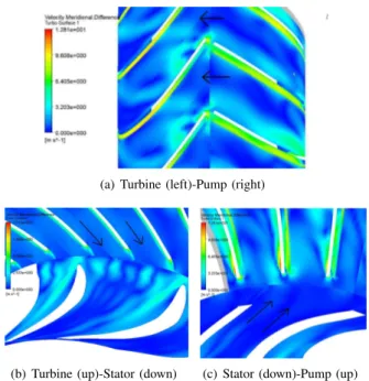
The localization of the unsteady effects was done by comparison between the steady and unsteady state. The com-parison in the chapter III-B of the nondimensional charac-teristics showed differences between the steady and unsteady calculations. However, the steady simulation means that the results only analyze the flow at a certain relative position in comparison with the unsteady calculation reproducing the variation in the flow as the position blade changes and take account the time-dependent effects. In this part of the work the steady and unsteady flow field will be compared for one relative position in order to locate the present unsteadiness. For this purpose, the Fig. 9 shows the meridional velocity difference∆Cm between steady and unsteady simulation.
(a) Turbine (left)-Pump (right)
(b) Turbine (up)-Stator (down) (c) Stator (down)-Pump (up)
Fig. 9. Meridional Velocity Difference ∆Cm between the Steady and Unsteady Flow Field at the Midspan Plane
simulation. It means that in the steady simulation the wakes at the interface will be transported downstream and find the turbine blades causing the upstream moving against the downstream flow from the pump exit. The highest differences at the turbine inlet occur in the area of the stagnation point. In the turbine passage the unsteady effects are small. However, in the suction side of the pump inlet and in the rotor-rotor interaction area these become significant.
At the turbine inlet the deviation increases due to the blade/row interaction. One physical effect that can be re-sponsible for this is a shock wave forming at the trailing edge which interacts with the vortex shedding process behind the blade. This phenomenon can be supported by observing a steady-state calculation that should not show this. In the unsteady simulation the flow must accelerate around the trailing edge much more than in the steady calculation in order to fill the wake. From this comparison, it is clear that the unsteady effects over the turbine suction surface are not equivalent to the effects on the pressure side of the blade. At the turbine inlet can be seen, that the mixing process of unsteady flow leaving the pump blade is strongly affected by the position of the pump that causes downstream conditions. We can come to the conclusion that the wakes of the downstream flow by the steady simulation will be clearly predicted larger than by the unsteady calculation. More information about the interaction area between the rotors can be obtained by the plotting of the meridional velocity fluctuation for relative positions of the pump and turbine.
B. Unsteady Simulation
The flow inside the H.T.C. is periodic in time (T=60∆t). First of all, it is known that the effects of these interactions depend on the number of blades (ZP = 31and ZT = 29).
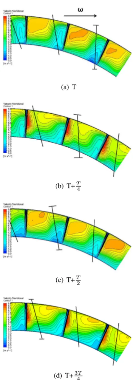
In this part of the paper the pump/turbine interface will be studied by analizing of the unsteady instantaneous meridional velocity (Cm) for four different relative pump/turbine
posi-tions of a period T at the pump exit and turbine inlet. The important problem here is how the flow information passes
(a) T
(b) T+T4
(c) T+T2
(d) T+34T
Fig. 10. Cm Contour Plot for One Period T at Turbine Inlet and Pump Blade Relative position (represented by black lines)
between two rotating blade rows. In Fig. 10 the unsteadyCm
distribution is shown in an axially constant contour plot at the turbine inlet located downstream of the pump. The objective here is to show the velocity distribution in the relative frame of reference of the turbine inlet for distinct relative positions of the pump. The contours show clearly three low velocity regions, which represent exactly the relative pump blade position in front of the turbine inlet. These low velocity areas are due the dcownstream effect of the wakes from the pump and the stagnation regions of the turbine. Here the superposition of the pump and turbine blade wakes take place. This interaction between the downstream pump wakes and the upstream turbine wakes seem to be the principal cause of the unsteady disturbances, which are directly related with pressure and torque oscillations (Fig. 7).
(a) T
(b) T+T4
(c) T+T2
(d) T+34T
Fig. 11. Cm Contour Plot for One Period T at Pump Exit and Turbine Blades Relative Position (black lines)
region in the passage.
The Fig. 11 shows the pump exit plane and the relative turbine blade positions for a cycle. A slightly periodically influence on the pump exit due to the aerodynamic blade row interactions can be observed. The position of the turbine blades causes only slightly unsteady effects and velocity decrease at the pump exit. The influence of the turbine will be reduced in direction of the pump pressure side. Due to the aerodynamic interactions of the blade rows the velocity distributions change considerably in time. For this reason unsteady blade forces and torques are generated. The principal cause of wake interaction is the downstream row that is directly influenced by the pitch ratio, the different rotating speeds, axial gap between components (proximity) and complex geometry. The main consequences of the growth of unsteadiness are the increase of the losses and on the other hand the increased loading of the blades with fluctuating forces, causing that the blades can be excited to vibrate.
V. CONCLUSION
The present paper shows the flow investigation of a torque converter. Comparing unsteady with steady calculations the
flow field having high frequency oscillations due to phenom-ena such as blade/wake interactions, very fine grids and small time steps as well as high computer resources are required. The computational resources time for unsteady flow are ten times higher than those for a steady.
Measurements verify the calculated global values obtained by CFD calculations. The results (Fig. 5) indicate that differences between steady and unsteady simulation occur significantly at low operating points. The torque conversion differs less than 4% over the operating area.
The results showed a 3D unsteady behaviour in the pump/turbine interaction area between incoming wakes and turbine passage structure. The wake area shows a wake struc-ture in the region at turbine inlet. The significant changes in velocity are induced by the relative position of the rotors. At the interaction region there is a superposition of the blade wakes (blade cutting), that causes an increase of theCm.
The turbine blade position have a little influence on the pump exit flow field, whereas the turbine inlet flow shows a significant periodic dependence on the relative pump blade positions. The change in velocity are induced by the relative motion of the rotors. It was noted that the rotor wakes at turbine inlet are stronger than those at pump exit. At the speed ratio ν=0.7 the downstream flow into the turbine passage is uniform and more forced against the blades than for lower speed ratios because of rotating velocity difference between pump and turbine. Because of that it is expected that more unsteadiness at lower speed ratios appear (Fig. 5).
REFERENCES
[1] A. Ruprecht. Unsteady Flow Analysis in Hydraulic Turbomachinery. Technical report, Institute of Fluid mechanics and hydraulic Machinery University of Stuttgart, Germany, May 2001. Invited lecture, Applied Industrial Fluid Dynamics, Aalborg.
[2] J. Schweitzer and J. Gandham. Computational fluid dynamics in torque converters: validation and application. International Journal of Rotating Machinery, 9:411–418, 2003.
[3] J. Park and K. Cho. Numerical flow analysis of torque converter using interrow mixing model. JSME International Journal, 41:847– 854, 1998.
[4] H. Schulz; R. Greim and W. Volgmann. Calculation of three dimen-sional viscous flow in hydrodynamic torque converter.ASME Journal of Turbomachinery, 118:578–589, 1996.
[5] Y. Kunisaki et al. A study on internal flow field of automotive torque converter: three dimensional flow analysis around a stator cascade of automotive torque converter by using PIV and CT techniques.JSAE, 22:559–564, 2001.
[6] A. Habsieger and R. Flack. Flow characteristics at the pump-turbine interface of a torque converter at extreme speed ratios. International Journal of Rotating Machinery, 9:419–426, 2003.
[7] T. Roecken; C. Achtelik and R. Greim. Stroemungsuntersuchung in hydrodyamischen Wandlern: Zusammenspiel von Messung und Rechnung. Forsch Ingenieurwes, 63:293–307, 1997.
[8] H. Foerster.Automatische Fahrzeuggetriebe: Grundlagen, Bauformen, Eigenschaften, Besonderheiten. Springer-Verlag Berlin et al., 1990. [9] Esso A.G. Bereich S.: Datenblatt ATF LT 71141. 1. Moorburger
Bogen 12, 1995. 21079 Hamburg.
[10] M. Giles. Calculation of unsteady wake/rotor interaction. J. Propul. Power, 4:356–362, 1988.
[11] B. Launder and D. Spalding. The numerical computation of turbulent flows. Computer Methods in Applied Mechanics and Engineering, 3:269–289, 1974.
[12] M. Wollnik; W. Volgmann and H. Stoff. Importance of the navier-stokes sorces on the flow in a hydrodynamic torque converter.WSEAS Transactions on Fluid mechanics, 5:363–369, 2006.
[13] M. Wollnik.Auswirkungen des Schaufelkanalverlaufs auf die Anteile hydrodynamischer Kraftuebertragung in Trilok-Drehmomentwandlern. PhD thesis, Ruhr-University-Bochum, 2008.