Development of a system for adsorption measurements in the 77 – 500 K and 1 – 100 bar range

(1)

Licenciado em Ciências da Engenharia Física

Development of a system

for adsorption measurements

in the 77 – 500 K and 1 – 100 bar range

Dissertação para obtenção do Grau de Mestre em

Engenharia Física

Orientador: Prof. Dr. Grégoire Bonfait,

Professor Associado com Agregação, Universidade Nova de Lisboa

Co-orientador: Dr. Daniel Martins, Thermal Engineer,

Active Space Technologies

Júri

Presidente: Dr. Filipe Tiago de Oliveira Arguente: Dr. Rui Ribeiro

(2)

(3)

in the 77 – 500 K and 1 – 100 bar range

A Faculdade de Ciências e Tecnologia e a Universidade NOVA de Lisboa têm o direito, perpétuo e sem limites geográficos, de arquivar e publicar esta dissertação através de exemplares impressos reproduzidos em papel ou de forma digital, ou por qualquer outro meio conhecido ou que venha a ser inventado, e de a divulgar através de repositórios científicos e de admitir a sua cópia e distribuição com objetivos educacionais ou de investigação, não comerciais, desde que seja dado crédito ao autor e editor.

Este documento foi gerado utilizando o processador (pdf)LA_{TEX, com base no template “unlthesis” [1] desenvolvido no Dep.}

(4)

(5)

First of all, I would like to thank my advisor, Prof. Grégoire Bonfait, for his guidance, commitment, for the opportunity provided to work in his laboratory and for helping me open the door to the field of Cryogenics. I must also extend these thanks to Daniel Martins, my co-advisor, who was always ready to help and contribute with valuable insight. It was an enriching experience to be a part of the project and the laboratory, both professionally and personally, and I can only hope to be a part of such a work dynamic in my future.

Also extremely helpful were the efforts and input of the members of the Laboratory of

Adsorption Technology and Process Engineering at the Chemistry Department: Prof. José Paulo Mota, who clarified the system design equations at an initial stage and provided a lot of data to discuss and compare with, and Isabel Esteves and Rui Ribeiro, with whom our discussions about adsorption always allowed us to improve our system and learn something more.

I must also thank my colleagues who were present at the Cryogenics Laboratory during my work, Jorge Barreto, Miguel Baeta, and Patrícia Borges de Sousa, for their constant availability, help, and great company in both serious and less serious contexts.

Our work would have been made much more complicated without the abilities of the department’s workshop and so thanks are extended to: João Faustino for the manufacturing of all the workshop-made pieces, and Eduardo Jobling for the brazing of both the gas manifold and the calibrated volume. Both are also thanked for their input.

To my girlfriend, Yen, for constantly pushing me to try harder, for listening to all my complaining, and for being an incredible inspiration. To my friends: Inês, my sincerest thanks for your infectious attitude, your company, and your constant encouragement; Francisco, for your friendship over the years, which will hopefully carry on even as we tread different paths in different places; Stella, for being a great friend all the way from

cold Latvia and for the constant shared laughter. And finally, a huge shout-out to all the TeamSpeak and Praça de Espanha field regulars, with whom the videogames and football meant a necessary break once in a while. All of you made these sometimes stressful months much lighter in different, equally valuable ways.

(6)

(7)

Adsorption is a phenomenon present in various systems important to the field of cryogenics, having a great deal of relevance in the development of vibration-free coolers: these are crucial for the cooling of sensitive detectors, as they offer the possibility of

using a sorption compressor, do not have moving parts and do not induce unwanted mechanical vibrations in the system, maintaining its sensibility and greatly minimizing wear due to use.

In the context of an ESA-funded project for the development of such a cooler, a study on adequate adsorption materials to use for the non-mechanical cryogenic compressor present in the final system was required. Considering this, a system for measurement of adsorption properties in the range of its operating pressures and temperatures was needed and, independently, also useful in future adsorption studies the laboratory decides to perform.

A brief historical and functional review of the adsorption phenomenon, its applications in cryogenics, and available and various methods for its measurement is made. The design and assembly of an adsorption measurement system, through the volumetric (also known as manometric) method, for temperatures in the 77 K to 500 K range and pressures up to 100 bar is detailed.

Proof pressure tests were made to validate the design of the vessel, with positive results. Other pre-measurement tests, such as heating and cooling assays, void and dead volume measurements, empty-vessel measurements, were all carried out with an intention to validate and characterize the developed system. A LabVIEWTMinterface for the control and automatic acquisition of the system parameters was developed and tested throughout the whole process.

Results were taken using a sample of HKUST-1 (also known as Cu3(BTC)2 or BasoliteTM _{C300) and compared against the results from another group, as well as a} partner laboratory, from both their theoretical simulations and their commercial gravimetric system.

(8)

(9)

A adsorção é um fenómeno utilizado em vários sistemas criogénicos, tendo grande relevância no desenvolvimento de vibration-free coolers: estes são cruciais para o

arrefecimento de detectores sensíveis, pois oferecem a possibilidade de uso de um compressor de sorção, não têm partes móveis e não induzem vibrações mecânicas indesejadas no sistema, mantendo a sensibilidade e minimizando significativamente o desgaste proveniente do uso.

No contexto de um projecto financiado pela ESA para o desenvolvimento de um criorrefrigerador deste tipo, um estudo sobre materiais adsorventes adequados para o uso no compressor criogénico não-mecânico presente no sistema final foi necessário. Tendo isto em consideração, um sistema para medida de propriedades de adsorção na gama de pressões e temperaturas de funcionamento do compressor foi necessário, e também útil em futuros estudos de adsorção que o laboratório efectue.

Uma breve revisão histórica e funcional do fenómeno de adsorção, as suas aplicações na criogenia, e os disponíveis e variados métodos para a sua medição é efectuada. O projecto e montagem de um sistema de medidas de adsorção, através do método volumétrico (também conhecido como manométrico), para temperaturas entre 77 K e 500 K e pressões até 100 bar, é detalhado.

Testes de pressão preliminares foram efectuados para validar o desenho da célula, com resultados positivos. Outros testes pré-medição, tais como ensaios de aquecimento e arrefecimento, medições de volumes mortos, medições sem amostra, foram efectuados com a intenção de validar e caracterizar o sistema desenvolvido. Uma interface em LabVIEWTM_{para controlo e aquisição automática dos parâmetros de todo o sistema foi} desenvolvida e testada durante todo o processo.

Foram obtidos resultados usando uma amostra de HKUST-1 (também conhecido como Cu3(BTC)2ou BasoliteTMC300) e comparados com os resultados de outro grupo e de um laboratório parceiro, tanto das suas simulações teóricas como do seu sistema gravimétrico comercial.

(10)

(11)

List of Figures xiii

List of Tables xvii

1 Introduction 1

2 Contextualization 3

2.1 Vibration-free cooler in the 40 – 80 K range . . . 3

2.2 Adsorption . . . 4

2.2.1 Types of adsorption . . . 5

2.2.2 Theoretical formulations . . . 7

2.2.3 HKUST-1 and other adsorbents . . . 9

2.2.4 Applications in cryogenics . . . 11

3 State of the art 17 3.1 Experimental methods . . . 17

3.1.1 Volumetric method . . . 17

3.1.2 Gravimetric . . . 18

3.1.3 Others . . . 20

3.2 Literature review of adsorption data on HKUST-1 . . . 20

4 Experimental setup 23 4.1 System summary and the volumetric method . . . 23

4.2 System dimensioning . . . 27

4.2.1 Wall thicknesses . . . 27

4.2.2 Adsorption vessel . . . 29

4.2.3 Calibrated volume . . . 32

4.3 Vessel filling and preparation . . . 33

4.4 LabVIEWTM_interface _{. . . .} ₃₅

4.5 Cooling and heating system . . . 36

4.6 Experimental procedure . . . 40

4.7 Determination of system volumes . . . 42

(12)

5 Results and analysis 47

5.1 Neon on HKUST-1 adsorption isotherms . . . 47

5.2 400 K to 500 K results. . . 53

5.3 Analysis. . . 54

5.3.1 Error and correction analysis . . . 54

5.3.2 Comparison with gravimetric data . . . 55

5.3.3 Isosteric heat of adsorption . . . 56

6 Conclusions 59

References 61

(13)

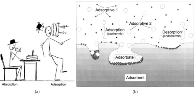
2.1 In (a), the difference between absorption and adsorption in layman’s terms. In

(b), an illustration of adsorption with two adsorbates (or “adsorptives”) and

an adsorbent surface. Both taken from [5]. . . 4

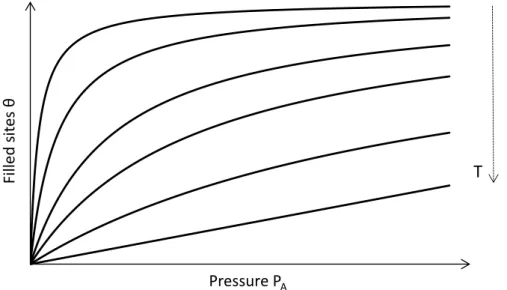
2.2 Example of typical Langmuir isotherms. For the same pressure, the highestθ signifies a lower temperature (as in, more adsorption at lower temperatures!). 7 2.3 In (a), activated carbon [14]. In (b), zeolite [15]. These are the two most used and commercialized types of adsorbents. . . 9

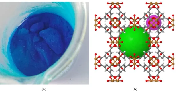
2.4 In (a), HKUST-1 in its powder form, as it is provided commercially. Note the darker and lighter hues of blue, corresponding to different states of oxidation (reversible). In (b), the molecular framework of HKUST-1, with spheres representing the pore sizes within it that can be used for gas storage. The green sphere has a diameter of approximately 10 Å. [20] . . . 10

2.5 Schematic of a generic Joule-Thomson cryocooler using adsorption compressors [1]. . . 11

2.6 Diagram of the project’s two-stage cryocooler. Adapted from [24]. . . 12

2.7 Working cycle of a 5 K Joule-Thomson cryocooler’s adsorption compressor, taken from [1]. . . 13

2.8 Vapour pressure vs. temperature for common pumped gases [25]. . . 14

2.9 Structure of a gas gap heat switch, adapted from [26]. . . 15

3.1 Typical volumetric method measurement system, adapted from [5]. . . 18

3.2 Typical gravimetric method measurement system, adapted from [5]. . . 19

3.3 Thermogravimetric analysis of HKUST-1 in an N2environment. Adapted from [31]. . . 21

4.1 Gas system of the built system. The Pt100 thermometer locations are given by letters A through D. . . 23

4.2 The densities in the system. . . 24

4.3 Two illustrative, mathematical examples of a bimodal packing [32]. . . 25

4.4 Representation of hoop stress, denominatedσ1[35]. . . 28

4.5 Representation of thread parameters:pthe pitch,Dthe major diameter andd the minor diameter [36]. . . 29

(14)

4.7 A 3D view of the support system. . . 30

4.8 In (a), the final version of the vessel. Note the smaller holes for Pt100 thermometers. In (b), the support system mounted on the manifold, to be compared to figure 4.7. . . 31

4.9 The calibrated volume, with the mounted thermometer C. . . 32

4.10 The vessel, post-filling. . . 33

4.11 Vestigial amounts of HKUST-1 outside the vessel. . . 33

4.12 In (a), the system for controlled soldering. Not shown is a glass wool cap on the top of the vessel to lower cooling by convection. Note the (good) final aspect of the solder bead. In (b), temperature vs. time for the process. . . 34

4.13 The vessel with its thermometers and heating resistor. A second layer of teflon was applied before the insulation to fix and protect the wiring. . . 34

4.14 The LabVIEWTMinterface’s main tab.. . . 35

4.15 From left to right, the first to final iterations of the vessel’s thermal insulation. 36 4.16 A diagram of the final version of the heating and cooling system, as seen inside the dewar. The vessel is protected by the glass wool and foam insulation from the liquid nitrogen, and held in place by the support system detailed in subsection 4.2.2. Not shown but implicit is the teflon protection from figure 4.13. The thermometers (A and B) and the heating cartridge (Heat) positions are represented. . . 37

4.17 An example of temperature stabilizations in the whole temperature range, lower in (a) and higher in (b), with a temperature slope criterion of 0.03%. Notice the heating peaks and following stabilization in temperature. The vessel was empty for these tests. . . 39

4.18 The manifold, fully wall mounted. Compare to figure 4.1 and note the support system described in subsection 4.2.2, figure 4.7, on the left after valve 5, as well as the insulation for the calibrated volume described in 4.2.3, after valve 4 in the bottom. . . 40

4.19 The method to go beyond the bottle’s pressure. . . 41

4.20 The volume designations in the system and their capacity, determined as explained in the text below. . . 42

4.21 A diagram of the method forV0. . . 43

4.22 The relative error of ideal vs. real (REFPROP) gas quantity in the vessel for several heating cycles done at circa 2 bar for the first, (a), and second, (b), silicon tries. . . 44

4.23 The silicone excess in the second round. . . 45

(15)

5.2 The total adsorption isotherms up to 400 K. Outlined is the set of results from figure 5.1 (b).. . . 50 5.3 The higher temperature isotherms not discernible in figure 5.2. . . 51 5.4 The points obtained using procedure B (crosses) overlapped with the total

results from figure 5.2. . . 52 5.5 In the dashed ellipse, the points taken after the 296 ºC soldering, with the

previous results. . . 53 5.6 Comparison between our 300 K and 340 K (ideal and real gas) isotherms with

the 303 K and 343 K isotherms from LATPE’s gravimetric apparatus. The eff_{ect of the real gas correction is noticeable.} _{. . . .} ₅₅

5.7 The isosthers calculated from the data of figure 5.2.. . . 56 5.8 Adsorption heat vs. adsorbed quantity, through equation 2.5 and figure 5.7. 56 5.9 Comparison between our experimental data, the experimental and simulation

(16)

(17)

2.1 Physical properties of BasoliteTMC300, adapted from [19]. . . 10

4.1 Variations of pressure between two extreme vessel temperature and system pressure cases (130 K, 16 bar to 500 K, 100 bar).. . . 27

(18)

(19)

C

h

a

p

t

e

1

I n t r o d u c t i o n

One of the most important applications of space cryogenics is the cooling of infrared detectors in satellites with a wide array of purposes. The recent years saw, in Europe, the development of active coolers that are capable of providing significant cooling power at an operational temperature of around 50 K, to meet Earth infrared observation mission requirements. In the case of missions for space observation, such as, for example, the Infrared Space Interferometer Darwin, these detectors enable the precise search of other Earth-like worlds and analysis of their biological properties, as well as other astrophysical objects in a similar wavelength range [1]. It’s within the optimization of these types of applications that the cooling of the detectors is of great importance. The most advantages are gathered by the so-called vibration-free coolers, cryocoolers that function without moving parts and so do not induce unwanted vibrations that negatively affect the infrared

detection system.

In general, the compressor is the biggest source of vibrations in a cryocooler: a vibration-free cooler must then invariably use a vibration-free compressor. A possibility is the use of a sorption compressor, which, as opposed to mechanical compressors, works thermochemically: this diff_{erence is enough to eliminate or minimize unwanted}

vibrations during its functioning. One of the researched options for this application is the use of this type of compressor to enable a Joule-Thomson effect. Such a

Joule-Thomson, vibration-free cryocooler is to be developed in a European Space Agency project. The objectives of this project are to design, manufacture and test what’s called anElegant Breadboard Modelof a vibration-free cooler that can provide active cooling for

(20)

This document will approach the work done in the design, development and testing of a system for adsorption measurements, with the intention to provide useful data on different adsorbent materials to aid the design and construction of an efficient adsorption

compressor for a vibration-free Joule-Thomson cooler. This dissertation is split into five other chapters.

In chapter2, the objectives of the work carried out and the project within which it is inserted are described. With an intention to lay the groundwork for an accurate understanding of the rest of the document, a general contextualization on the adsorption phenomenon and its different types, theories and applications in the field of cryogenics,

with an emphasis on cryocoolers, is exposed, as well as a description of the sample used to validate the system.

In chapter3, an overview of the various experimental methods for the measurement of adsorption properties, as well as a literature review pertaining to the most recent and pertinent adsorption results to the developed system are carried out.

In chapter4, the most important aspects of the volumetric experimental setup that was developed are explored. After an initial summary of the layout and its key components, the dimensioning - from general design to volumes and thicknesses, considering the high pressures reached - is detailed for all these components: the adsorption vessel and the calibrated volume, as well as the cooling and heating system designed to cover the 77 K to 500 K range. The preparation of the vessel and the sample prior to mounting in the system is explained. A brief description of the LabVIEWTM interface is also given, highlighting the automatic stabilization algorithm and the data acquisition system. Also included in this chapter are step-by-step descriptions of the experimental procedures, as well as an overview of the helium measurements of the system’s volumes, which are fundamental for a later result analysis. A small section on the empty-vessel tests carried out with an aim to pre-validate the system elaborates on experiments made without an adsorbent sample, in an attempt to confirm the volumes present in the system by performing routine measurements.

In chapter 5, the results for adsorption of neon on HKUST-1 are presented, most notably in the form of adsorption isotherms, from which important data such as the isosteric curves, the heat of adsorption, and others can be derived. A quantitative error and correction analysis is performed to gauge possible sources of error or corrections and their influence. Our results are compared with those obtained by a commercial gravimetric system belonging to LATPE, a partner laboratory in the Chemistry Department, and with results for adsorption heat obtained by another group in 2013, as a means to validate our system.

Finally, in chapter6, general considerations and conclusions taken from this work, as well as what to improve about the system in the near future.

(21)

C

h

a

p

t

e

2

C o n t e x t u a l i z a t i o n

2.1 Vibration-free cooler in the 40 – 80 K range

In 2014, the European Space Agency posted anAnnouncement of Opportunitydetailing

specified requirements for the “Development of a 40 K to 80 K vibration-free cooler”. This project was assigned to two companies, one of them being Active Space Technologies: a Portuguese company specialized in thermo-mechanical and electronics engineering for aerospace, defense, automotive, nuclear fusion and scientific applications. It is currently in progress in collaboration with the Cryogenics Laboratory and the Adsorption Technology Group (LATPE), both located in the Faculdade de Ciências e Tecnologia of the Universidade Nova de Lisboa (FCT-UNL). From it originated a Ph. D. thesis (J. Barreto, for the development of a functioning prototype), and two M. Sc. theses (adding to this one, M. Baeta, for the development of the nitrogen stage).

The cooler is projected to be of the Joule-Thomson type, split in two stages, one with nitrogen and another with neon (cooling power: 0.5 W at 80 K and 40 K, respectively). It’s predicted to cover most of the 40 K to 80 K range. To avoid the vibration induced by the more common mechanical compressors used for gas compression, the compressor will be sorption-based. Advantages of the latter are discussed in a later section about cryocoolers.

(22)

tendency to adsorb. A brief description of the adsorbent is available in a later section.

2.2 Adsorption

Adhesion of any atoms, ions, or molecules provenient from a fluid to a surface is defined as adsorption. The process creates a layer of adsorbate on the adsorbent, at surface level. This phenomenon can be explained by the existence of a negative surface energy, which is the driving force behind any surface phenomena: in a material, the surface atoms, which are not wholly surrounded by other adsorbent atoms, are more susceptible to binding with surrounding bodies due to this unbalanced and asymmetric configuration in comparison to the bulk atoms. The attracted particle (adsorbate) then fills in the pores on the surface of the solid (adsorbent) when this phenomenon occurs. It’s worth noting that surface energy caused by atomic force imbalance is not the only factor for the characterization of adsorption properties, as the compatibility of pairs of adsorbents and adsorbates (usually called adsorption working pairs) is defined by several other properties [3], [4].

(a) (b)

Figure 2.1: In (a), the difference between absorption and adsorption in layman’s terms. In

(b), an illustration of adsorption with two adsorbates (or “adsorptives”) and an adsorbent surface. Both taken from [5].

The term sorption encompasses both adsorption and absorption: differences between

both lie in the fact that absorption involves permeation or dissolution of the absorbate in the absorbent, involving then the bulk of the material, as opposed to adsorption, which involves only the surface.

(23)

way to put it is to look at the equation for the Gibbs free energy,G, a thermodynamical potential that’s minimized at chemical equilibrium at constant temperature and pressure: that means a diminishing Gsignifies a spontaneous, or favored, reaction. This potential was described by its eponym, J. W. Gibbs, as:

... the greatest amount of mechanical work which can be obtained from a given quantity of a certain substance in a given initial state, without increasing its total volume or allowing heat to pass to or from external bodies ... [6]

Its general definition is:

G(P, T) =H−T S (2.1)

whereGis the Gibbs free energy,P the pressure,T the temperature,Hthe enthalpy, andSthe entropy, all pertaining to aclosedsystem.

So, at constant temperature:

∆_G=∆_H₋_T∆_S (2.2)

Saying adsorption is exothermic is the same as saying the variation of enthalpy,∆_H, associated with adsorption is negative. Moreover, since the adsorption of a gas implies the restriction of its movement, an adsorption intuitively leads to a decrease in the entropy of the gas, and thus∆_Sis negative. For the process to be spontaneous, or∆_Gnegative, seeing as ∆_S is negative,∆_H must be necessarily negative enough to cancel out the positive

−T∆Sterm. Therefore, adsorption is generally exothermic, always for physisorption in

particular but not necessarily for certain variants of chemisorption, however [7]. These two types of adsorption will be explained in subsection that follows.

2.2.1 Types of adsorption

Adsorption processes are mostly distinguished by the nature of the bonding processes involved, being usually characterized as chemical adsorption (or chemisorption) or physical adsorption (or physisorption). The distinction is basically the same as one between general chemical and physical interactions, and is sometimes difficult to make

(24)

2.2.1.1 Chemisorption

In this type of adsorption, the adsorbate reacts chemically with the adsorbent, becoming chemically bonded with it: this means that the chemical structure of the material’s surface is altered, so generally only one layer – a monolayer – of a given adsorbate will form. It’s a very selective process, depending heavily on the chemical nature of both adsorbent and adsorbate. The forces involved have a very short range, as characteristic of chemical bonds. Also to note is that this process is often irreversible, making it impossible to remove the adsorbed gas without altering the surface. Chemisorption has extremely high bond enthalpies: between 250 kJ/mol and 500 kJ/mol. In general, this very large enthalpy makes the use of this type of adsorption not viable for adsorption compressors. This is the main difference to physisorption.

2.2.1.2 Physisorption

Unlike chemisorption, physisorption occurs when the adsorbate remains on the adsorbent’s surface due to weak, long-range Van der Waals or London forces. Since the binding energies involved are relatively weak (less than 20 kJ/mol), it’s heavily influenced by temperature and pressure of the system: since physisorption is an exothermal process, low temperatures and high pressures contribute to adsorption, while high temperatures and low pressures lead to desorption. Due to the long-range of the forces and the non-chemical nature of these processes, it’s possible to have multilayered adsorption as long as the forces involved allow it.

Within the context of this thesis, physisorption will be the sole focus, and so any mentions of adsorption from this point on refer to the physical, and not the chemical, type.

(25)

2.2.2 Theoretical formulations

To this date, at least 15 different isotherm models have been developed for adsorption

studies. They have varying degrees of ideality and sophistication, as well as different

cases in which they are applicable or not [10].

One of the simplest and most versatile models to date was derived by Langmuir, in 1918. This adsorbate-adsorbent system was treated by making several assumptions:

• The adsorbate behaves as an ideal, classical gas;

• The adsorbent surface is perfectly flat and homogeneous;

• The adsorbate becomes immobile after adsorbing;

• All the adsorption sites are equivalent;

• There are no interactions between adsorbed molecules.

The system is basically treated as a chemical system – though the reaction is not necessarily chemical – with reactions occurring for adsorption and desorption. The reagents are considered the free adsorbate molecules and the open adsorbent sites, and the products the adsorbent’s occupied sites. Equalizing the chemical potentials of these two states, the central equation for the Langmuir model can be derived, which gives the percentage of filled adsorbent sitesθas a function of the gas pressurePA:

θ= KPA

1 +KPA (2.3)

whereK is a constant, dependent on reaction heat, particle mass and temperature. Equation2.3leads to the so-called Langmuir isotherms of adsorption, figure2.2:

0 0.1 0.2 0.3 0.4 0.5 0.6 0.7 0.8 0.9 1

0 20 40 60 80 100

Fi

ll

e

d s

it

es

θ

Pressure P_A

T

(26)

It’s interesting to note that the isotherms for high temperatures (which would be the lower adsorbed quantities θin figure 2.2) exhibit a linear behavior with respect to pressure, while the isotherms for lower temperatures, where adsorption is more favored, exhibit much earlier saturation. This saturation reduces the effect of pressure at high

pressures, as the adsorbent material’s sites are then almost completely filled with the adsorbate gas. At low pressures, θ is proportional to P_A, which is called Henry’s Law. This experimental law is confirmed by the limit of low pressure of the Langmuir model.

To understand the adsorption process, it’s also important to know that it results in dynamic equilibrium: a coexistence of free molecules and adsorbed molecules, where both adsorption and desorption are constantly happening at the same rate. This can be described by equation2.4, where the rates of adsorption and desorption are equaled:

K= Ka Kd =

[AB]

[A][B] →K= θ

(1−θ)PA (2.4)

where [A] is the quantity of free gas molecules (proportional toP_A), [B] the quantity of unoccupied surface atoms (proportional to 1−θ) and [AB] the quantity of adsorbed

gas molecules (proportional toθ).KaandKd are the rates of reaction of adsorption and

desorption, respectively. Rearranging equation2.4, we obtain the former equation2.3. This model is widely used, both educationally and experimentally: it is applicable in most chemisorption phenomena as well as physisorption below a given saturation pressure, giving it versatility. Other models that take, for instance, multilayers (Brunauer-Emmett-Teller, or BET for short, often used to estimate adsorbent surface areas [11]), larger incidence of adsorption near already adsorbed molecules (Kisliuk [12]), and other factors into account, exist for applications where a higher degree of analysis is required.

Another important theoretical aspect is the calculation of the heat of adsorption. As already mentioned, adsorption leads to a dynamic equilibrium, and is an exothermal process, which means a molecule of gas transfers heat to its surroundings when it is adsorbed. By treating adsorption as a change of phase and the gas as ideal, we can apply the Clausius-Clapeyron equation to calculate the reaction heat (equation2.5) [13]:

L=−Rδ(ln(P))

δ_T1 (2.5)

where L is the reaction heat, R the ideal gas constant, P the pressure and T the temperature of the system.

One important thing to keep in mind is that, in the specific case of adsorption,Lis conventionally taken at isosteric conditions, meaning at constant adsorbed quantities θ.

Essentially, the slope of an isosteric curve, which would be a horizontal line in figure2.2, plotted with ln(P) and _T1, will give us the adsorption heat. This slope should be negative, as we concluded earlier from∆_Hin equation2.2.

(27)

2.2.3 HKUST-1 and other adsorbents

Currently used adsorbents can be split into several categories, depending on their typical surface area (which is always relatively large) and their intended and diverse applications: these can be industrial, medical, scientific, among others.

(a) (b)

Figure 2.3: In (a), activated carbon [14]. In (b), zeolite [15]. These are the two most used and commercialized types of adsorbents.

The most widely popular and commercialized adsorbent in cryogenics is activated carbon, a form of carbon processed in such a way that it has small, low-volume pores that give the material an enormous surface area: typically around 1000 m2/g and as high as 3000 m2_{/g [5]. The raw carbon is extracted from common carbonaceous materials} such as nutshells, wood, and coal. The extraction is often called carbonization, and is performed through pyrolisis (thermochemical decomposition of organic materials in an inert environment) in the temperature range from 600 ºC to 900 ºC. The carbon product’s surface area is then enhanced through physical or chemical means, called activation. In the physical case, this means exposure to an oxidizing atmosphere at very high temperatures (600 ºC to 1200 ºC), while in the chemical case, it means impregnation of the raw material with certain strong chemicals. A convenient property of activated carbon is that it has a great variety of heavily researched methods for its regeneration, such as ultrasound [16], electrochemical [17] and microwave-assisted [18] methods, not necessarily requiring high temperatures to desorb all the gas it holds.

(28)

HKUST-1, the material used to make measurements with the developed system, is an adsorbent categorized as a metal-organic framework and available under the commercial name BasoliteTM _{C300, manufactured by Sigma Aldrich (Germany). Its chemical} denomination is Cu3(BTC)2. Table 2.1 summarizes and highlights some interesting properties as an adsorbent of this commercialized variant of HKUST-1.

Table 2.1: Physical properties of BasoliteTM_{C300, adapted from [19].}

Property HKUST-1

Activation conditions 423 K under vacuum (10 h) Molecular weight 605 g/mol

Particle size 16 µm

Bulk density 350 kg/m3

BET surface area 1500 to 2100 m2/g

This material was one of options for the project’s adsorption compressors due to its capacity in adsorbing both nitrogen and neon better than activated carbon. As already mentioned in section2.1, adsorbing neon is conventionally less favorable: this is due to its little or no ability to react when compared to non-noble gases. It was tested on due to its quick availability when compared to the other analyzed metal-organic frameworks, that were both not commercial and not simple to synthesize.

(a) (b)

Figure 2.4: In (a), HKUST-1 in its powder form, as it is provided commercially. Note the darker and lighter hues of blue, corresponding to different states of oxidation

(reversible). In (b), the molecular framework of HKUST-1, with spheres representing the pore sizes within it that can be used for gas storage. The green sphere has a diameter of approximately 10 Å. [20]

(29)

2.2.4 Applications in cryogenics

2.2.4.1 Cryocoolers

Adsorption is usually not the concept directly behind any type of cooling. However, it can be used in several types of cooling cycles through sorption-based compressors [22], where the pressure cycles are generated through heating and cooling cycles of adsorbent-filled containers, generally called adsorption vessels. These compressors have the advantage that they do not have any moving parts, which severely minimizes their vibrations and wear due to use: this makes them attractive for a great variety of applications, where lifetime and the lowest possible level of vibrations are an important factor [23], such as in the project in which this thesis is inserted.

Figure 2.5: Schematic of a generic Joule-Thomson cryocooler using adsorption compressors [1]a_.

a_{Reprinted from Cryogenics, Vol. 42, nr. 2, J. F. Burger et al, Vibration-free 5 K sorption cooler for ESA’s}

For example, within the scope of the already mentioned project, the functioning of a Joule-Thomson sorption cooler (figure2.2.4.1) will be detailed to illustrate the importance of the compressor and its control.

As the name suggests, a Joule-Thomson cryocooler takes advantage of the Joule-Thomson effect to cool a working fluid. This effect, also known as a throttling

(30)

The equation that determines the Joule-Thomson coefficient that rules over this

phenomenon is as follows:

µJT = ∂T_∂P

!

H

= V

C_p(αT −1) (2.6)

In which µJT is the Joule-Thomson coefficient, T, P and H the gas temperature,

pressure and enthalpy, respectively, V the volume, Cp the heat capacity at constant

pressure, andαthe thermal dilation coefficient of the fluid. As it represents the variation

of temperature with pressure of an isenthalpic process, a positive Joule-Thomson coefficient yields a cooling with expansion: the pressure decreases, and thus the

temperature must decrease. A negative Joule-Thomson coefficient results in heating: the

pressure decreases, and thus the temperature must increase. The variation of this coefficient’s signal leads to the so-called inversion temperature, _T_inv: above this

temperature, the coefficient is always negative, while below it, it is positive. Hydrogen,

helium and neon have inversion temperatures lower than 300 K at atmospheric pressure, requiring then some pre-cooling in order to take advantage of the Joule-Thomson effect.

Figure 2.6: Diagram of the project’s two-stage cryocooler. Adapted from [24].

(31)

constant presences in these cryocoolers to facilitate pre-cooling and increase the cooler efficiency, as well as any other heat transfers present in the system. Despite being a part

of the project, these elements will not be discussed in detail within this thesis, as they are not present in the developed adsorption measurement system (M. Baeta, M. Sc. thesis).

Sorption compressors are cyclical systems in which the adsorption vessels alternate between adsorption and desorption (respectively, lowering and raising pressure) through the variation of temperature. As already mentioned in the description of physisorption, temperature has a strong influence in these phenomena. However, to avoid strong fluctuations of gas flow, which are harmful to the temperature stability of the Joule-Thomson cycle, one needs at least four vessels, functioning out-of-phase with each other, with adequate check valves [1].

(a) (b)

Figure 2.7: Working cycle of a 5 K Joule-Thomson cryocooler’s adsorption compressor, taken from [1] a_{. In (a), the cycle drawn over generic adsorption isotherms. In (b), the}

variation of the several system parameters over the cycle.

a_{Reprinted from Cryogenics, Vol. 42, nr. 2, J. F. Burger et al, Vibration-free 5 K sorption cooler for ESA’s}

(32)

limit (in the example, 1 bar), the valve opens, which establishes a flow of adsorbing gas entering the vessel from the expansion valve in a fourth phase, D. Two pairs of vessels operating in opposed phase manage to damp the flow fluctuations inherent to this cycle.

2.2.4.2 Cryopumps

In the field of vacuum technology, cryopumps are a constant presence in high and ultra-high vacuum systems. They are clean, fast vacuum pumps that work through removal of gases and vapors through condensation and adsorption on cold surfaces.

Condensation of particles on the cold surface happens when the vapor pressure of a given gas at the given cold temperature is so low that the condensed phase forms, effectively removing the gas particle from the system’s volume. Unfortunately, the

condensation of neon, hydrogen and helium is impossible with most cryopumps, because the vapor pressure of the former two at 20 K (the temperature limit for a relatively simple and usual cryocooler) is considerably high and the liquid phase for helium appears only below 5 K. The adsorption of these gases, however, doesn’t suffer

from this temperature limitation, which makes it a very good complement to the condensation process, making this a relatively effective pump for all types of gases, yet

with some limitations for helium.

Figure 2.8: Vapour pressure vs. temperature for common pumped gases [25]a

a_{Reprinted from Vacuum, Vol. 30, nr. 30, P. D. Bentley, The modern cryopump, pp. 145–158, Copyright}

1980, with permission from Elsevier.

(33)

occur for an infinite number of particles, or an infinite amount of time, without “cleaning out” the system: this process, called regeneration, involves the warming of the cryopump to a high temperature, allowing the trapped gases and vapours to go back to a gaseous state, being then removed from the system by the appropriate pumping system.

2.2.4.3 Heat switches

As their name suggests, heat switches are devices with the capability to switch as needed between a high and a low thermal conductance state. Many types of heat-switches exist, but the gas gap heat switch is where adsorption plays a major role. It’s nowadays in use for some satellites where cryogenics take part due to its peculiar, advantageous characteristics in space conditions: it is both compact and without moving parts when actuated by a cryopump.

Figure 2.9: Structure of a gas gap heat switch, adapted from [26]a_.

a_{Reprinted from Cryogenics, Vol. 48, nr. 1, I. Catarino et al, Neon gas-gap heat switch, pp. 17–25,}

(34)

(35)

C

h

a

p

t

e

3

S t a t e o f t h e a rt

3.1 Experimental methods

To dimension a system, the characteristic adsorption isotherms (for instance, figure 2.2.4.1, bottom left,X(T , P)) must be known. It is on this topic that a small overview of adsorption measurement methods currently in use is done in this chapter, with historic contextualization and current developments in each of them. The overview on experimental methods is based heavily on [5].

3.1.1 Volumetric method

The volumetric (or manometric) method is considered the pioneer of adsorption measurements, with early experiments situated in the late 1700s up to the early 1900s. A prototype of what is the current typical setup was developed and established in the 1940s.

It consists on the principle that if a given quantity of gas is well known, it can be expanded into a pre-evacuated vessel with an adsorbent sample in it. As the expansion is carried out, the quantity of gas is split into partially adsorbed on the adsorbent and partially remaining in the proximity of the adsorbent in a gaseous state. Through conservation of mass and knowledge of the void volume (the volume in which the adsorbate gas can enter), the amount of gas being adsorbed can be calculated.

(36)

on the particularities of the system. This change in gas quantity is the adsorbed quantity, as adsorbed particles don’t contribute to gas pressure. Because the pressure measurement is the key of this determination, the name “manometric” is also conventionally used.

A typical experimental setup for this method is displayed in figure3.1.

Figure 3.1: Typical volumetric method measurement system, adapted from [5].

What’s remarkable about this method is that it is in many ways simple and effective, as

a measurement is done by opening a valve and measuring a final pressure in the system, which makes it convenient for the programming of an acquisition system. It also gives the user complete temperature control, as the sample can be mounted on a cold source without any hindrances. The disadvantages are that there should be enough adsorbent in the vessel, usually several grams, for a pressure variation to be discernible — this can be an issue when the quantity of sample available is low or when it is relatively expensive — and that the pre-determination of the void volumes and the calibrated volume should be as accurate as possible to obtain accurate measurements, which implies that the existence of unknown volumes must be minimized. There has to be a compromise between the calibrated volume, the vessel volume (and so the adsorbent material quantity) and the amount of gas initially in the system for the variation in pressure to be measurable. This is the method for which the final system was dimensioned and the specifics of its application will be further detailed in chapter4.

3.1.2 Gravimetric

(37)

restraints. The gravimetric method as it is applied today, concerning adsorption phenomena of gases on solids, is then relatively recent, from the second half of the 1900s.

The method is based on the fact that an adsorbent on which an adsorbate accumulates undergoes a variation in mass, equal to the mass of the adsorbed gas. Thanks to noticeable improvements of weighing techniques and microbalance quality, this method is nowadays very sensitive. Within the gravimetric methods, different variants can be distinguished,

dependent on the type of balance used, whether the balance is a single or double beam type, and the temperature region exploited.

Figure 3.2: Typical gravimetric method measurement system, adapted from [5].

(38)

3.1.3 Others

Several other recent methods exist besides the two aforementioned ones, with varying levels of popularity and divulgation. Again, most of this subsection is mainly based on [5].

Volumetric-gravimetric systems are systems in which the two previously described methods are applied simultaneously, in order to both conjugate the advantages of the two and to be able to determine coadsorption equilibria of gas mixtures without requiring a chromatograph or mass spectrometer. They are specially applied to industrial process control and design.

The oscillometric method, or oscillometry, consists of a pendulum or a freely floating rotator in slow rotational oscillation, coated with adsorbent material, where the damping of the movement of the chosen structure in a surrounding adsorbate is due to both the adsorption phenomenon and the friction with the gas. Measurements can be made optically, to gauge the movement properties of the structure in use. The chamber is in a thermostatic bath, which brings the same disadvantage as the gravimetric method: lack of good sample temperature control.

The impedance spectroscopy method relies on the basis that, if a static or alternating electric field is applied to a weakly electrical conducting or dielectric material — which encompasses most activated carbons, materials typically used for adsorption studies — the electrons and nuclei of the components are shifted in opposite directions to each other. This induces dipole moments in the material, which are measurable through the capacitance C or impedance Z of capacitors filled with the material in question. One gets C(f) or Z(f) curves, where f is the frequency of the applied electric field, which are characteristic for the adsorbent material in vacuum and for adsorbent/adsorbate systems. Through pre-calibration with the aid of other methods, such as manometric or gravimetric, one can obtain a curve that relates capacitance or impedance to quantity of adsorbed gas. This makes impedance spectroscopy also highly automatable, sharing the rest of the advantages and disadvantages of gravimetry.

3.2 Literature review of adsorption data on HKUST-1

In this section, there is a succinct review of published work done by other groups that is pertinent to our goals. This means, essentially, volumetric measurements in high temperature and pressure conditions compared to the usual range, performed in HKUST-1.

(39)

lesser performances for neon and nitrogen adsorption. Chan, C.K.et al, however, shared our goal of application in adsorption compressors, and thus covered a large range of temperatures and pressures (77 K to 400 K, 1 atm to 80 atm).

More recently, in 2011, Moellmer, J.et alalso treated high-pressure adsorption (up to

500 bar), this time for HKUST-1, using however a much smaller temperature range (273 K to 343 K) [28]. These were, at the time, reported to be the first high-pressure (over200 bar) measurements done on this sample. As explained in the paper’s introduction and to further explain the lack of extensive literature on this topic, most of HKUST-1’s current applications lie in the lower pressure range: at the time of publishing and to the best of their knowledge, the only other literature found for high pressure adsorption measurements on HKUST-1 was a volumetric and gravimetric analysis of methane adsorption in a group of metal-organic frameworks [29], going up to 200 bar.

In 2013, an interesting study on noble gas adsorption in HKUST-1, experimental and computational [30], provides us with values for adsorption heats for neon adsorption, with which we’ll compare our results in addition to the ones simulated and obtained by LATPE in subsection5.3.3.

In 2014, Raganati, F.et alanalyzed CO2capture in HKUST-1 in a sound assisted bed [31], having in parallel confirmed several physical properties. The most interesting in our perspective was a thermogravimetric analysis which gives us a reasonable profile of the behavior of the material with temperature, giving us an absolute maximum temperature limit of circa 350 ºC (see figure3.2). This motivated us to perform a thermogravimetric analysis to confirm their results, since the temperature maximum is of great importance to our measurements and the soldered sealing of our vessel (see section4.3).

Figure 3.3: Thermogravimetric analysis of HKUST-1 in an N2 environment. Adapted from [31]a_.

a_{Reprinted from Chemical Engineering Journal, Vol. 239, F. Raganati et al, CO}

2capture performance of

(40)

(41)

C

h

a

p

t

4 E x p e r i m e n t a l s e t u p

4.1 System summary and the volumetric method

As mentioned in the former chapter, the volumetric method was chosen for our measurements. A diagram summarizing the developed system is displayed in figure4.1.

Vessel

Dewar Calibrated _volume Gas bottle

Pressure

sensor 2 Pressure sensor 1

Vvessel

V2

2

5 1

V1

V0

Vacuum pump

E

3 4

B

A

C D

Figure 4.1: Gas system of the built system. The Pt100 thermometer locations are given by letters A through D.

(42)

calibrated volume V2, used as a buffer and for the initial gas quantity determination. Also connected to the manifold are the gas bottle, from which the sample adsorbate is provided, and a rotary vacuum pump, for cleaning out the whole system.

Valves 1 and 2 are used for the supply of gas, 1 being the adjustable supply, so we can establish a given initial pressure, and 2 a quarter-turn valve. Valve 3 is the pumping valve, and valve E the escape valve, opened in the case of a non-pumpable pressure excess in the system. Valves 4 and 5 constitute the interface between the calibrated volume and the adsorption vessel. Operation of this manifold will be further discussed in section4.6.

The expression that rules over the system is the mass balance at a given equilibrium pressure and system temperatures:

Nvessel(P, TA/B) =Ntotal−NV2(P, TC)−NV1(P, TD)−NV0(P, TD) (4.1)

whereNtotal is the total number of molecules in the system,Nvessel the total number

of molecules in the vessel (adsorbed or in a gaseous state),N_V_x (x= 0,1,2) the number of molecules in the several non-vessel volumes in the system, for a system pressureP, and the several system temperatures T_X (X =A, B, C, D), as per the designations of the thermometers in figure4.1.

N_vessel can then be used to determine the adsorbed quantity in the vessel, knowing

some other parameters that are explained below:

Nvessel(P, TA/B) =Vvessel

ǫρg(P, TA/B) + (1−ǫ)ρpq∗(P, TA/B)

(4.2)

whereVvessel is the vessel’s volume, ǫ the packing factor, ρg the gas density at the

vessel’s temperature and pressure,ρ_p the particle density, andq∗the specific adsorbed

quantity.

packing density

particle density

Figure 4.2: The densities in the system.

There are two densities referring to the material in this model, so a description of each is needed, with the help of figure4.2: ρp, the so-called particle density, is the

mass density of a single particle (its weight divided by its apparent volume) and so it takes into account the porosity that adsorbent materials have (see in the figure, zoomed in) and is often a material-specific constant.

ρb, the so-called packing density, is

(43)

of the particle, but also the inter-particle space (figure 4.2) that an imperfect packing inevitably has.

ρb=

m_adsorbent Vvessel

(4.3)

The packing factor,ǫ, tells us what fraction of the vessel corresponds to inter-particle space, which is not filled by adsorbent. In essence, a perfect packing (ǫ= 0) would yield a packing density equal to the particle density, as no interparticle space would exist:

ǫ= 1− ρ_b ρp

(4.4)

We can now look at equation4.2and understand the two terms: the first, multiplied byǫ, refers to the portion of the vessel not filled by adsorbent, or the space between each adsorbent particle, while the second, multiplied by 1−ǫ, refers to the portion filled by

adsorbent, in which adsorption occurs at a quantityq∗.

The smaller this packing factor, the more adsorbent was packed into a container of a given volume, which is attractive and very important in larger-scale projects due to volume and budget restraints. There are, however, theoretical limits depending on the distribution of particle sizes. Packing can be defined based on the number of distinct particle sizes present, from equally sized particles (monomodal), two differing sizes

(bimodal), and so on (multimodal). An example of bimodal packing can be seen in figure4.1.

(a) (b)

Figure 4.3: Two illustrative, mathematical examples of a bimodal packing [32]a_.

America Chemical Society.

(44)

the used method due to the fact that the quantity of adsorbent can simply be separated in half – one half is crushed, being then reduced to a much smaller grain, and the other half is unaffected, creating two different particle sizes – and because this simple process

increases the packing density by a significant quantity [34].

Rearranging equation4.2and using equation4.1, we can obtain the adsorbed quantity in terms of the system parameters:

q∗(_{P, T} A/B) =

Ntotal−NV2(P, TC)−NV1(P, TD)−NV0(P, TD)

V_vessel −ǫρg(P, TA/B)

(1−ǫ)ρp

(4.5)

(45)

4.2 System dimensioning

Dimensioning of the main components of the system — the adsorption vessel and the calibrated volume — has to take into account the measurement method in use and the extreme conditions when in operation.

The adsorption vessel and the calibrated volume must have dimensions such that the system’s pressure variation over the course of a measurement is measurable by the pressure sensors. Essentially, the initial quantity of gas in the calibrated volume has to expand sufficiently into the adsorption vessel so that a significant pressure variation is

detected. This creates a compromise: the calibrated volume has to be larger than the adsorption vessel and void volumes, but it cannot be so large that it requires an impracticable quantity of gas for a substantial pressure variation to be read. Using simulated data for neon adsorption on HKUST-1, calculated by J. P. Mota [21], an Excel worksheet was made to gauge this compromise, calculating the pressure difference

between two extreme vessel temperatures and system pressures with the results presented in table4.1.

Table 4.1: Variations of pressure between two extreme vessel temperature and system pressure cases (130 K, 16 bar to 500 K, 100 bar).

Vvessel/cm3 Vcal/cm3 mads/g ∆P/bar

7.5 150 4 4.62

7.5 1500 4 0.46

Looking at table 4.1, the values of 7.5 cm3 and 150 cm3 were decided on: the pressure variation of approximately 5 bar should be sufficient to carry out the

experiment, considering the sensitivity of the pressures sensors used.

4.2.1 Wall thicknesses

The fact that the system will have to hold in pressures up to 100 bar makes it so that some factors that would otherwise be irrelevant become critical — one in particular is the thickness of the walls of the constituents: the adsorption vessel, the involved tubes and the calibrated volume. Failure to accommodate such pressures can result in yield or even fracture of the constituent materials, which could compromise the setup in several ways. A strength study, implemented in an Excel worksheet, was made on the thickness of walls for cylindrical pressure vessels with hemispherical caps — this shape was chosen due to its structural resilience — applying the thin-wall and thick-wall approaches. The thin-wall approximation assumes that the cylinder walls are infinitely thin in comparison to the diameter, and so it is appliable when the thickness of the wall can be considered sufficiently small in comparison to the diameter. Regardless, we concluded

(46)

approximations on wall thickness are made. For the thin-wall approximation, the highest stress on a cylinder under internal pressure is the hoop stress,σθ, given by [35]:

σθ=

Pr

t (4.6)

whereP is internal pressure,r the radius of the cylinder, andt the thickness of its walls. This stress is also called circumferential, because it occurs along the circumference of the cylinder’s walls.

Figure 4.4: Representation of hoop stress, denominatedσ1[35].

The expression for the thickness is then direct, from equation4.6:

t=Pr

σ_θ (4.7)

where, taking into account a limit hoop stress equal to the yield strength of the material in use (as in, the tension required to have the material go into the plastic regime of strain), one can obtain a safe thickness for the cylinder walls of a given material, radius and working pressure. The pressure taken into account was 200 bar, despite the maximum working pressure being 100 bar. This, combined with a security factor of 2 (which gives us a combined safety factor of 4!), is enough to guarantee that the cylinder walls will hold up at the desired working pressures. These calculations were done for every custom part in our setup. For the commercial pieces, such as the tubing and the valves, they were chosen so that their pressure limits largely fulfill our requirements.

(47)

4.2.2 Adsorption vessel

The two initial ideas were to either have disposable adsorption vessels or a reusable one with a screw-on cap. The screw would then be tightened and filled with soft solder so as to become leak-tight even at high pressures. The latter idea was opted for, and thus a more detailed strength study was made for the screw in the cap, to determine the thread parameters (figure4.5) that allowed for large pressures.

Figure 4.5: Representation of thread parameters: pthe pitch,Dthe major diameter and d the minor diameter [36].

The stress on one given screw can be calculated as (F is the force,Sthe surface):

σ_screw₁=F S=

4F

π(D2−d2) (4.8)

With the stress distributed over a given numberN of screws being:

σscrews=

σscrew1

N =

p H

4F

π(D2−d2) (4.9)

A regular thread of 1 mm pitchpover 10 mm lengthHproved no issue, with a stress of 6.8 MPa in comparison to the usual approximate yield strength of copper, 70 MPa.

To validate this design, a dummy vessel (slightly shorter than the final version) was built to perform a burst pressure test with water, using a high pressure generator and a pressure sensor (up to 300 bar). Let us note that this test was done with water for safety reasons: a gas burst is much more destructive than a water burst, due to the higher compressibility of gases.

The copper dummy vessel had a radius of 9 mm, and consequently, according to equation 4.7, a wall thickness of around 5 mm. The test also had the intent to test out the hypothesis that the vessel should hold under pressures of 200 bar, for which it was dimensioned.

(48)

Figure 4.6: The dummy vessel built for pressure testing.

considered finished, with positive results: the vessel holds up in pressures at least almost three times as high as the maximum working pressure of around 100 bar!

Figure 4.7: A 3D view of the support system. After this design was considered validated in terms of

pressure, the drawing of the final version was possible. There were a few changes compared to the dummy vessel: the vessel was made longer to increase its volume to the projected 7.5 cm3 from table 4.1, holes were made to tightly accommodate both the 50 W heating resistor and the two Pt100 thermometers, and a support system was designed to hold the vessel to the gas manifold, protect the thin capillary that connected the two, and allow the wiring of the vessel resistors to the room-temperature adapter. The final version can be seen in figures4.7(which will be described below) and4.8(b).

A stainless steel tube (2) was brazed on one extremity to the brass piece that’s screwed on top of the vessel (1), and on the other to a 12-pin connector adapter (4) for the temperature controller. This allowed us to wire the thermometers and heater mostly through this tube, greatly protecting the wiring.

To add on to this, an aluminum piece (3) was manufactured to hold the capillary’s manifold connection to the stainless steel tube, as well as fix the whole support system to the manifold (see figure4.8(b)).

Why a very thin capillary? Since the vessel temperature is going to vary between 77 K and 500 K and the manifold will be always at room temperature, there will often be a very large temperature gradient in the capillary connecting the vessel to the manifold: a minimization of this volume to the point that it is almost negligible will reduce possible errors in the calculation of its gas quantity. The capillary that was mounted in the system

(49)

doesn’t necessarily mean that it doesn’t factor into calculations – an average temperature between the vessel and the manifold was taken for this volume and considered in the final calculations, despite having little effect in the results.

(a) (b)

Figure 4.8: In (a), the final version of the vessel. Note the smaller holes for Pt100 thermometers. In (b), the support system mounted on the manifold, to be compared to figure4.7.

The volume of this final vessel (figure 4.8, (a)) was then measured to confirm our initial projection. The measurements were done by weighing the vessel, both completely empty and completely filled with distilled water, and taking the difference as the mass

of water inside. This can then directly be converted to the volume of water inside. The drawing had a volume of 7.634 cm3, while the measurement yielded 7.63 cm3, leading us then to conclude that we could use this value as a constant for the rest of the work to

(50)

4.2.3 Calibrated volume

One solution initially thought out for the calibrated volume was the acquisition of a diving cylinder. These diving cylinders withstand up to 300 bar and typically have an internal volume of 3 to 18 L. However, no compatible sizes were commercially available considering the projected dimensions in table4.1.

Figure 4.9: The calibrated volume, with the mounted thermometer C.

The calibrated volume was able to be manufactured in our workshop, from a 316 stainless steel rod, which saved us time and resources. The drawing was done to obtain a piece that would hold, as per table4.1, around 150 cm3_{. Considering the usable length of material} we had, the determined inner radius for the volume was 21 mm, which brought the thickness to (again, as per equation 4.7) around 4 mm. The length was calculated to be 108.3 mm. It’s interesting to notice how much stronger stainless steel is than copper: a vessel with more than double the radius has 20% less thickness for the same pressure requirements due to the relatively higher yield strength. The piece was made in three separate parts: the body, and two caps to be brazed on each side, so as to close the hollow cylinder. A 1/4 inch tube with a standard connector was then brazed to the holed cap so that the calibrated volume could be connected to the gas manifold. An attempt at measuring the volume through water weight was made after all pieces of the calibrated volume were welded. Unfortunately, the complete filling of the volume with water through the small tube proved more complicated than initially predicted, as air bubbles could be heard as it was shaken and the volume results were highly variant and lower than initially predicted. In hindsight, a suitable solution would be to have done this prior to the brazing of the top cap, which would simplify the filling. The final capacity measurement had to then be performed through gas expansion, section4.7.

(51)

4.3 Vessel filling and preparation

For the adsorption vessel to be ready for the introduction of the sample, mounting of the resistors and soldering of the cap (a process which was repeated several times over the course of this work), it must be thoroughly clean. This was done initially by hand to remove any obvious moisture and finalized with an ultrasonic bath, set to 10 minutes using acetone. This cleaning procedure is important for the inner part of the vessel, which will be in contact with the sample, but also for the outer threaded part, in order to allow a good wetting of the screw to be soldered.

Figure 4.10: The vessel, post-filling. Filling the vessel with HKUST-1 has to be a careful process,

as the material is toxic and ours had a very small grain size of 16 µm (see table 2.1), meaning it behaved almost like very light dust. Thus, protective equipment such as glasses, gloves and a dust mask are advised, as well as careful handling. The material doesn’t seem to adhere at all to paper, which makes it a suitable base to carry out the filling. The greatest possible amount of adsorbent has to be put into the vessel, which requires mechanical vibrations by hand on the vessel as the filling is done, to force the sample to fully settle (as best as possible) in the free space beneath it. Further compression was made with a metal piece to attempt a greater degree of packing. The vessel was weighed before and after this process to determine the mass of sample that had been packed into it.

Figure 4.11: Vestigial amounts of HKUST-1 outside the vessel.

To prevent the sample from leaving the vessel as pumping or fast gas discharges occur, some type of filter had to be applied. The choice fell on a stainless steel grid with 25 µm holes as well as a small quantity of glass wool in the tube exiting the vessel’s cap. This quantity of glass wool is crucial, as an initial experiment with only the aluminum grid had us discover that the sample left the vessel quite easily (figure4.11, in light blue). This forced us to clean out the system, as we had pumped a small quantity of sample.

The cap is then tightly screwed on and the complete vessel exposed to a pre-activation period in order to remove unwanted moisture from the sample. After staying overnight at 80 ºC in a low vacuum, the muffle

(52)

(a) 0 50 100 150 200 250 300

0 10 20 30 40 50 60

Temp er a tu re / oC

Time / min

(b)

Figure 4.12: In (a), the system for controlled soldering. Not shown is a glass wool cap on the top of the vessel to lower cooling by convection. Note the (good) final aspect of the solder bead. In (b), temperature vs. time for the process.

Figure 4.13: The vessel with its thermometers and heating resistor. A second layer of teflon was applied before the insulation to fix and protect the wiring.

This soldering process, in the case of high-temperature solders (above 250 ºC), has to be controlled due to the sensibility of HKUST-1 to temperatures above 300 ºC (see figure 3.2). With this in mind, a small set-up for a well-controlled and uniform soldering process was made (figure 4.12), which allowed for a high degree of control and for the process to be done in less than 10 minutes, which is positive because the sample was only at high temperatures for a relatively short time.

After this, the thermometers and heating resistor can be mounted in the vessel and isolated electrically with teflon tape (melting point: 600 K) (figure4.13). The designations for the thermometers in the figure are identical to the ones in figure4.1.

(53)

4.4 LabVIEW

TM

interface

The system’s interface was developed in LabVIEWTM_{, adapted from a previous interface} already implemented by Gonçalo Tomás for thermal conductivity measurements of porous copper [37].

Figure 4.14: The LabVIEWTM interface’s main tab.

Its function is to provide a visualization of the important parameters such as pressure, heating power and all the mounted thermometers’ readings, as well as some other features: automatic acquisition, temperature control, result and log file output and pressure vs. temperature graphs for real-time analysis, allowing early detection of possible system anomalies.

The aspect that is less trivial and more interesting to note is the equilibrium detection algorithm: it calculates the slope of a given number of acquired points and constantly compares it to a stabilization criterion set by the user. In our case, it does this for both temperature and pressure, the parameters that should be constant at an equilibrium, acquiring a given number of points that satisfy these criteria in a row. Then, when the designated number of stable points is uninterruptedly obtained, they’re registered in a file and an increment to the controller’s temperature setpoint occurs, leading the interface to then repeat the process at another temperature point.