Rita Cristina Pinto de Sousa
Mestre em Estatística
Parameter Estimation
in the Presence of Auxiliary Information
Dissertação para obtenção do Grau de Doutora em Estatística e Gestão de Risco, Especialidade em Estatística
Orientador :
Sat Gupta, Professor of Statistics,
University of North Carolina at Greensboro, USA
Co-orientador :
Pedro Corte Real, Professor Auxiliar,
Universidade Nova de Lisboa, Portugal
Júri:
Presidente: Prof. Doutora Maria Luísa Dias de Carvalho de Sousa Leonardo
Arguentes: Prof. Doutor Dinis Duarte Ferreira Pestana
Prof. Doutora Maria Teresa Themido da Silva Pereira
Vogais: Prof. Doutor João Tiago Praça Nunes Mexia Prof. Doutora Célia Maria Pinto Nunes Prof. Doutor Sat Gupta
iii
Parameter Estimation
in the Presence of Auxiliary Information
Copyright cRita Cristina Pinto de Sousa, Faculdade de Ciências e Tecnologia, Universi-dade Nova de Lisboa
Acknowledgements
The last four years were a great challenge for me. I have to thank many people who made this interesting journey possible. Their scientific or emotional support was crucial to reach the end of my thesis.
• First of all I would like to thank my Mentors, the advisor Sat Gupta and the co-adviser Pedro Corte Real for sharing their great knowledge and experience with me. I have to point out their tremendous support and their orientation ability that made me easily forget and overcome the physical distance.
I thank Professor Pedro Corte Real especially for having encouraged me to invest in my school graduation which contributed to my growth as a researcher. His friendly receptivity, the sharing of his knowledge and his great ideas were fundamental for my motivation and for a better outcome. His experience and friendship are for me an important and true reference.
I thank Professor Sat Gupta especially for sharing with me his pleasure, knowledge and motivation in working on this theme. The chance to work with him allowed me to meet many people, to learn a lot and take a broad view of estimation with auxiliary information. He proved to be a very friendly person. I consider him an excellent reference as person, as a mentor and as a researcher.
I am deeply grateful to them. Their support greatly contributed for my develop-ment as research and as person.
• I would like to thank the Professors and people from the university staff who sup-port the post-graduate students. A special thanks to the coordinator Manuel Es-quível for his support and his incentive to carry on, always understanding my con-straints as working student.
• I would like to thank all my Co-Authors who helped me write the chapters of this thesis. Their collaboration improved and expanded my knowledge on several top-ics.
viii
experience and to Nursel for being a good reference as a young and active re-searcher.
• I also would like to thank the anonymous referees for making very constructive suggestions which resulted in a significant improvement over the original version of the papers to be found in the chapters of this thesis.
• Thanks to my work colleagues for their support and encouragement.
A special reference to Pedro and São, my classmates at Statistics Portugal, for their advice and for having always a friendly word encouraging me and giving me strength to carry on.
A special message of affection to my colleagues from afrolatINE for having always supported me and for having contributed to my well being and happiness. Who dances is happier.
• Thanks to my parents and my sister for their affection and unconditional support. From the beginning my parents always supported me, encouraging me in my de-cision and doing everything they could to allow me to complete successfully this journey. They are my true inspiration.
My sister is a true example of a blood sister and especially a sister by heart. Thank you for being as you are.
Abstract
In survey research, there are many situations when the primary variable of interest is sensitive. The sensitivity of some queries can give rise to a refusal to answer or to false answers given intentionally. Survey can be conducted in a variety of settings, in part dic-tated by the mode of data collection, and these settings can differ in how much privacy they offer the respondent. The estimates obtained from a direct survey on sensitive ques-tions would be subject to high bias. A variety of techniques have been used to improve reporting by increasing the privacy of the respondents.
The Randomized Response Technique (RRT), introduced by Warner in 1965, develops a random relation between the individual’s response and the question. This technique provides confidentiality to respondents and still allows the interviewers to estimate the characteristic of interest at an aggregate level.
In this thesis we propose some estimators to improve the mean estimation of a sensi-tive variable based on a RRT by making use of available non-sensisensi-tive auxiliary informa-tion. In the first part of this thesis we present the ratio and the regression estimators as well as some generalizations in order to study the gain in the estimation over the ordinary RRT mean estimator. In chapters 4 and 5 we study the performance of some exponential type estimators, also based on a RRT. The final part of the thesis illustrates an approach to mean estimation in stratified sampling. This study confirms some previous results for a different sample design. An extensive simulation study and an application to a real dataset are done for all the study estimators to evaluate their performance. In the last chapter we present a general discussion referring to the main results and conclusions as well as showing an application to a real dataset which compares the performance of study estimators.
Keywords: Auxiliary variable; Exponential estimator; Randomized response technique;
Resumo
Em estudos de pesquisa por inquérito existem muitas situações em que a variável de interesse é sensível. A sensibilidade de algumas questões pode dar origem a recusas na resposta ou a falsas respostas dadas de forma intencional. Os inquéritos podem assumir diversas configurações, em parte relacionadas com o método de recolha e com o grau de privacidade que é oferecido aos respondentes. As estimativas obtidas por inquérito direto em questões sensíveis estariam sujeitas a erros elevados. Muitas técnicas têm sido utilizadas para melhorar as respostas através do aumento de privacidade dos inquiri-dos. A Técnica de Resposta Aleatorizada, introduzida por Warner em 1965, desenvolve uma relação aleatória entre as respostas individuais e a questão. Esta técnica providencia confidencialidade aos respondentes e ainda permite aos entrevistadores estimar a carac-terística de interesse num nível mais agregado.
Nesta tese propõem-se alguns estimadores para melhorar a estimação da média de uma variável sensível baseada numa técnica de resposta aleatorizada com recurso a in-formação auxiliar disponível não sensível. Na primeira parte da tese apresentam-se os estimadores da razão e da regressão bem como algumas generalizações para estudar o ganho na estimação face ao estimador ordinário da média. Nos capítulos 4 e 5 estuda-se a performance de alguns estimadores do tipo exponencial, também baseados numa téc-nica de resposta aleatorizada. A parte final da tese ilustra uma aproximação à estimação da média com amostragem estratificada. Este estudo vem confirmar resultados anterio-res com um novo desenho amostral. Um extenso estudo de simulação e uma aplicação a dados reais são feitos para avaliar a performance de todos os estimadores. No último capítulo apresenta-se uma discussão geral, bem como uma aplicação a dados reais onde se compara a performance dos estimadores em estudo.
Palavras-chave: Estimador da razão; Estimador da regressão; Estimador exponencial;
Contents
Contents xiii
List of Figures xv
List of Tables xvii
Listings xix
Abbreviations xxi
1 General Introduction 1
References . . . 3
2 Ratio Estimation of the Mean of a Sensitive Variable in the Presence of Auxil-iary Information 5 Abstract. . . 5
2.1 Introduction . . . 6
2.2 Terminology . . . 6
2.3 The Proposed Estimator . . . 7
2.4 A Simulation Study . . . 9
2.5 Numerical Example . . . 11
2.6 Transformed Ratio Estimators . . . 13
2.7 Conclusions . . . 18
References . . . 18
xiv CONTENTS
3 Estimation of the Mean of a Sensitive Variable in the Presence of Auxiliary
In-formation 31
Abstract. . . 31
3.1 Introduction . . . 32
3.2 Terminology . . . 32
3.3 The Ratio Estimator . . . 33
3.4 Ordinary Regression Estimator . . . 34
3.5 Generalized Regression-cum-ratio Estimator . . . 35
3.6 The Simulation Study. . . 37
3.7 Numerical Example . . . 39
3.8 Conclusions . . . 41
References . . . 41
Appendix B - R Routines . . . 43
4 Exponential Type Estimators of the Mean of a Sensitive Variable in the Presence of Non Sensitive Auxiliary Information 49 Abstract. . . 49
4.1 Introduction . . . 50
4.2 Terminology . . . 50
4.3 Estimators Review . . . 51
4.4 Proposed Exponential Type Estimators. . . 52
4.5 Comparison with Gupta et al. (2012) Estimators . . . 55
4.6 Simulation Study . . . 56
4.7 Numerical Example . . . 58
4.8 Conclusions . . . 60
References . . . 60
Appendix C - R Routines . . . 63
5 Improved Exponential Type Estimators of the Mean of a Sensitive Variable in the Presence of Non-Sensitive Auxiliary Information 71 Abstract. . . 71
5.1 Introduction . . . 72
CONTENTS xv
5.3 Difference-cum-exponential Estimator (Koyuncu et al., 2013) . . . 73
5.4 Proposed estimator . . . 73
5.5 Simulation Study . . . 75
5.6 Numerical Example . . . 77
5.7 Conclusions . . . 79
References . . . 79
Appendix D - R Routines . . . 81
6 Improved Mean Estimation of a Sensitive Variable Using Auxiliary Information in Stratified Sampling 89 Abstract. . . 89
6.1 Introduction . . . 90
6.2 Terminology . . . 90
6.3 Estimators Review . . . 91
6.4 Proposed combined ratio estimator . . . 92
6.5 Proposed combined regression estimator . . . 94
6.6 A Simulation Study . . . 95
6.7 Numerical Example . . . 98
6.8 Conclusions . . . 100
References . . . 100
Appendix E - R Routines . . . 103
7 General Discussion 113 7.1 Summary . . . 113
7.2 Comparison of the main study estimators . . . 113
7.3 Final Remarks . . . 117
References . . . 118
List of Figures
7.1 Distribution of empiricalBias . . . 115
List of Tables
2.1 EmpiricalARBfor RRT mean estimator and ratio estimator (bold). . . 10
2.2 TheoreticalARBfor ratio estimator based on1stand2ndorder (bold) approximation. . . 10
2.3 MSEcorrect up to1stand2ndorder approximations and
PREfor the ratio estimator rela-tive to the RRT mean estimator. . . 11
2.4 EmpiricalARBfor the RRT mean estimator and the ratio estimator (bold). . . 12
2.5 TheoreticalARBfor the RRT mean estimator and the ratio estimator. . . 13
2.6 MSE, corrected to1storder approximation, and
PREfor the ratio estimator related to the RRT mean estimator. . . 13
2.7 EmpiricalARBfor the RRT mean estimator, the ratio estimator and for the transformed ratio estimators.. . . 15
2.8 TheoreticalARBto1storder approximation for the RRT mean estimator, the ratio estimator
and for the transformed ratio estimators. . . 16
2.9 EmpiricalMSEand theoretical (bold)MSEto1storder of approximation for the RRT mean
estimator, the ratio estimator and for the transformed ratio estimators.. . . 17
2.10 PREfor the transformed ratio estimator related to the ratio estimator based on1storder of
approximation. . . 18
2.11 Calculations for the expression in (2.16). . . 18
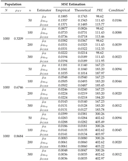
3.1 MSEcorrect up to1storder approximation and
PREfor the ratio estimator (µˆR), the
regres-sion estimator (µˆReg) and the generalized regression-cum-ratio estimator (µˆGRR) relative
to the RRT mean estimator. . . 38
3.2 MSEcorrect up to1storder approximation and
PREfor the ratio estimator (µˆR), the
regres-sion estimator (µˆReg) and the generalized regression-cum-ratio estimator (µˆGRR) relative
xx LIST OF TABLES
4.1 EmpiricalMSE, theoretical MSE correct up to1storder approximation and
PREof all esti-mators. . . 57
4.2 Table 4.1 Continued. . . 58
4.3 MSEandPREfor the ratio estimator (µˆR), the regression estimator (µˆReg), the generalized
regression-cum-ratio estimator (µˆGRR) and the exponential estimator (µˆexp1) relative to the
RRT mean estimator. . . 60
5.1 EmpiricalARBfor the difference-cum-exponential estimator (µˆDE) and for the improved
exponential estimator (µˆIE). . . 76
5.2 TheoreticalARBfor the difference-cum-exponential estimator (µˆDE) and for the improved
exponential estimator (µˆIE). . . 76
5.3 Empirical and theoreticalMSEfor the difference-cum-exponential estimator (µˆDE) and for
the improved exponential estimator (µˆIE). . . 77
5.4 EmpiricalARBfor the difference-cum-exponential estimator (µˆDE) and for the improved
exponential estimator (µˆIE). . . 78
5.5 TheoreticalARBfor the difference-cum-exponential estimator (µˆDE) and for the improved
exponential estimator (µˆIE). . . 78
5.6 Empirical and theoreticalMSEfor the difference-cum-exponential estimator (µˆDE) and for
the improved exponential estimator (µˆIE). . . 79
6.1 Empirical and TheoreticalMSE, for the RRT mean estimator, ratio estimator (underlined) and regression estimator (bold); and correspondingPRErelative to the RRT mean estimator. 97
6.2 Empirical, theoreticalMSE,PREfor the ratio estimator (underlined) and for the regression estimator (bold) relative to the RRT mean estimator andPREfor the simple random sample (SRS) relative to the stratified sample (Str). . . 99
7.1 TheoreticalARBfor the estimators in comparison. . . 115
7.2 EmpiricalMSE, theoreticalMSEcorrect up to1storder approximation and
Listings
2.1 R Code for Simulation Study of Proposed Estimator in Chapter 2 . . . 21
2.2 R Code for Simulation Study of Transformed Ratio Estimators in Chapter 2 24
2.3 R Code for Numerical Example of Proposed Estimator in Chapter 2 . . . . 28
3.1 R Code for Simulation Study of Proposed Estimator in Chapter 3 . . . 43
3.2 R Code for Numerical Example of Proposed Estimator in Chapter 3 . . . . 46
4.1 R Code for Simulation Study of Proposed Estimator in Chapter 4 . . . 63
4.2 R Code for Numerical Example of Proposed Estimator in Chapter 4 . . . . 67
5.1 R Code for Simulation Study of Proposed Estimator in Chapter 5 . . . 81
5.2 R Code for Numerical Example of Proposed Estimator in Chapter 5 . . . . 85
6.1 R Code for Simulation Study of Proposed Estimator in Chapter 6 . . . 103
6.2 R Code for Numerical Example of Proposed Estimator in Chapter 6 . . . . 108
List of Abbreviations
ARB- Absolute Relative Bias
Deff - Design Effect
ICT- Information and Communication Technologies
MES- Monthly Economic Survey
MSE- Mean Square Error
NACE- Statistical Classification of Economic Activities in the European Community
PRE- Percent Relative Efficiency
RRT- Randomized Response Technique
SRS- Simple Random Sample
SRSWOR- Simple Random Sampling Without Replacement
1
General Introduction
One of the major problems in survey research involving sensitive questions is the social desirability response bias (Edwards, 1957). For various reasons individuals in a sample survey may prefer not to confide to the interviewer the correct answers to certain ques-tions. In such cases the individuals may elect not to reply at all or to reply with incorrect answers. The resulting evasive answer bias is ordinarily difficult to assess. That bias is potentially removable through allowing the interviewer to maintain privacy using a randomization device (Warner, 1965).
Randomized response is a research method used in structured survey interview. It was first proposed by Warner in 1965 and later modified by Greenberg et al. in 1969. This technique allows respondents to respond to sensitive issues while maintaining confiden-tiality. It provides confidentiality to respondents through a random relation between the individual’s response and the question. It still allows the interviewers to estimate the characteristic of interest at an aggregate level.
Gupta and Thornton (2002) showed that Randomized Response Technique (RRT) is effective in circumventing the social desirability response bias, and is more friendly and portable than other methods such as the method which uses a bogus pipeline (Jones and Sigall, 1971).
scrambled response depending on whether the respondents find the question sensitive or not.
In RRT work, generally the focus is on the estimation of the mean of a sensitive vari-able or the prevalence of a sensitive characteristic in the population. The mean can be estimated by using one of many RRT but we propose some estimators which improve the mean estimation considerably by using non-sensitive auxiliary information. In such cases, one will be able to observe an auxiliary variable directly but will have to rely on some RRT to collect information on the variable of interest, resulting from a sensitive is-sue. Given that our main aim is to evaluate the performance of the mean estimator in the presence of auxiliary information, we opt for using an additive Full RRT method to scramble the sensitive variable.
The main goal of this thesis is to improve the parameter estimation of a sensitive variable in the presence of auxiliary information. For that purpose we introduce some estimators for the population mean based on the additive Full RRT technique. Expres-sions are derived for theBiasand Mean Square Error (MSE) for all the proposed estima-tors. Furthermore, an extensive simulation study and an application to a real dataset are done for all the study estimators. All the applications are developed using the statistical software R [1].
This thesis is based on five papers to be found in chapters 2–6. Each chapter presents, at least, a new estimator and evaluates its performance comparing it to the other estima-tors previously proposed. The contents of this thesis are as follows:
• InChapter 2we propose a ratio estimator for the mean of a sensitive variable using information from a non-sensitive auxiliary variable. We generalize the proposed estimator to the case of transformed ratio estimators. We show that there is hardly any difference in the first order and second order approximations forMSEeven for small sample sizes. We also show that the proposed estimator does better than the ordinary RRT mean estimator which does not use the auxiliary information (Sousa et al., 2010).
• In Chapter 3we introduce a regression estimator which performs better than the ratio estimator even for modest correlation between the primary and the auxiliary variables. We consider a generalized regression-cum-ratio estimator that has even smaller MSE. It is shown that the proposed regression estimator performs better than the ratio estimator and the ordinary RRT mean estimator that does not utilize the auxiliary information (Gupta et al., 2012).
• InChapter 4we propose exponential type estimators using one and two auxiliary
the proposed exponential type estimators are more efficient than the existing es-timators described in Sousa et al. (2010) and Gupta et al. (2012)(Koyuncu et al., 2013).
• InChapter 5we propose an improved exponential type estimator which is more efficient than the Koyuncu et al. (2013) estimator, which in turn was shown to be more efficient than the usual mean estimator, ratio estimator, regression estimator, and the Gupta et al. (2012) estimator. It is shown that the improved difference-cum-exponential estimator can produce further improvement relative to other esti-mators previously proposed (Gupta et al., 2013).
• InChapter 6we extend the ratio and regression estimators to the stratified sampling setting. Although both the ratio and regression estimators perform better than the ordinary RRT mean estimator, the improvement is much larger with the regression estimator. The results agree with the findings of Sousa et al. (2010) and Gupta et al. (2012) in simple random sampling. We show that the advantage of using the RRT in the presence of auxiliary information still holds in the context of stratified sampling (Sousa et al., 2013).
• InChapter 7we present a general discussion referring to the main results and con-clusions. We present a study with a real dataset and we show the numerical results for theBiasandMSE, as well as graphic evidence which illustrates the performance of the main study estimators.
In the last part of each chapter we attach the R routines developed for the simulation studies and for the numerical examples.
References
EDWARDS, A. L. 1957. The social desirability variable in personality assessment and research, New York: Dryden, Praeger.
EICHHORN, B. H. & HAYRE, L. S. 1983. Scrambled randomized response methods for obtaining sensitive quantitative data. Journal of Statistical Planning and Inference, 7, 307-316.
GREENBERG, B., ABDUL-ELA, A., SIMMONS, W. & HORVITZ, D. 1969. The unrelated question randomized response model: theoretical framework. Journal of American Statis-tical Association, 520-539.
Sensitive Variable in the Presence of Auxiliary Information. Communications in Statistics -Theory and Methods, 41(13-14), 2394-2404.
GUPTA, S., SHABBIR, J., SOUSA, R. & REAL, P. C. 2013. Improved exponential type estimators of the mean of a sensitive variable in the presence of non-sensitive auxiliary information. (submitted)
GUPTA, S. & THORNTON, B. 2002. Circumventing social desirability response bias in personal interview surveys. American Journal of Mathematical and Management Sciences, 22, 369-383.
JONES, E. E. & SIGALL, H. 1971. The Bogus Pipeline: A New Paradigm for Measuring Affect and Attitude.Psychological Bulletin, 76, 349-364.
KOYUNCU, N., GUPTA, S. & SOUSA, R. 2013. Exponential type estimators of the mean of a sensitive variable in the presence of non-sensitive auxiliary information. Communi-cations in Statistics - Simulation and Computation. (accepted).
MANGAT, N. S. & SINGH, R. 1990. An Alternative Randomized Response Procedure. Biometrika, 77, 439-442.
SOUSA, R., GUPTA, S., SHABBIR, J. & REAL, P. C. 2013. Improved Mean Estimation of a Sensitive Variable Using Auxiliary Information in Stratified Sampling. Journal of Statistics and Management Systems. (submitted).
SOUSA, R., SHABBIR, J., REAL, P. C. & GUPTA, S. 2010. Ratio estimation of the mean of a sensitive variable in the presence of auxiliary information. Journal of Statistical Theory and Practice, 4(3), 495-507.
WARNER, S. L. 1965. Randomized response: a survey technique for elimination evasive answer bias.Journal of American Statistical Association, 60, 63-69.
2
Ratio Estimation of the Mean of a
Sensitive Variable in the Presence of
Auxiliary Information
Abstract
We propose a ratio estimator for the mean of sensitive variable utilizing information from a non-sensitive auxiliary variable. Expressions for theBiasand Mean Square Error (MSE) of the proposed estimator (correct up to first and second order approximations) are de-rived. We show that the proposed estimator does better than the ordinary Randomized Response Technique (RRT) mean estimator that does not utilize the auxiliary informa-tion. We also show that there is hardly any difference in the first order and second order approximations forMSEeven for small sample sizes. We also generalize the proposed estimator to the case of transformed ratio estimators but these transformations do not result in any significant reduction inMSE. An extensive simulation study is presented to evaluate the performance of the proposed estimator. The procedure is also applied to some financial data (purchase orders (sensitive variable) and gross turnover (non-sensitive variable)) in 2009 for 5090 companies in Portugal from a survey on Information and Communication Technologies (ICT) usage.
2.1. Introduction
2.1
Introduction
In survey research, there are many situations when the primary variable of interest (Y) is sensitive and direct observation on this variable may not be possible. However, we may be able to directly observe a highly correlated auxiliary variable (X). For example,Y may be the number of abortions a woman might have had in her life andXmay be her age. SimilarlyY may be the total purchase orders in a year for a company andXmay be the total turn-over for that company in that year. In such cases, one will be able to observeX
directly but will have to rely on some Randomized Response Technique (RRT) to collect information onY. In such situations, mean ofY can be estimated by using one of many randomized response techniques but this estimator can be improved considerably by utilizing information from the auxiliary variableX. Many authors have presented ratio estimators when bothY andXare directly observable. These include Kadilar and Cingi (2006), Turgut and Cingi (2008), Singh and Vishwakarma (2008), Koyuncu and Kadilar (2009) and Shabbir and Gupta (2010).
Also, many authors have estimated the mean of a sensitive variable when the primary variable is sensitive and there is no auxiliary variable available. These include Eichhorn and Hayre (1983), Gupta and Shabbir (2004), Gupta et al. (2002), Saha (2008) and Gupta et al. (2010).
In this paper, we propose a ratio estimator where the RRT estimator of the mean of
Y is further improved by using information on an auxiliary variableX. Expressions for the Bias and MSEfor the proposed estimator are derived, correct up to both the first order and second order approximations. It is shown that the two approximations are very similar even for moderate sample size. We also observe that there is considerable reduction inMSEwhen auxiliary information is used, particularly when the correlation between the study variable and the auxiliary variable is high.
2.2
Terminology
LetY be the study variable, a sensitive variable which cannot be observed directly. Let
X be a non-sensitive auxiliary variable which is strongly correlated with Y. Let S be a scrambling variable independent of Y and X. The respondent is asked to report a scrambled response forY given byZ =Y +Sbut is asked to provide a true response for
X. Let a random sample of sizenbe drawn without replacement from a finite population
U = (U1, U2, ..., UN). For the ith unit (i = 1,2, ..., N), let yi andxi respectively be the values of the study variableY and auxiliary variableX. Moreover, lety¯ =
Pn i=1yi
n ,x¯ = Pn
i=1xi
n andz¯ = Pn
i=1zi
n be the sample means andY¯ =E(Y), X¯ =E(X) andZ¯=E(Z) be the population means forY,X andZ, respectively. We assume thatX¯ is known and
¯
2.3. The Proposed Estimator
E(δi) = 0,i=z, x.
If information onXis ignored, then an unbiased estimator ofµY is the ordinary sam-ple mean(¯z)given by (2.1) below
ˆ
µY = ¯z. (2.1)
The mean square error (MSE) ofµˆY is given by
M SE(ˆµY) =
1−f
n S
2
y+Ss2
, (2.2)
where
f =n/N,Sy2 = N1
−1 PN
i=1(yi−Y¯)2,Sx2 = N1−1 PN
i=1(xi−X¯)2andSs2= N1−1 PN
i=1(si−S¯)2.
2.3
The Proposed Estimator
We propose the following ratio estimator for estimating the population mean of the study variableY using the auxiliary variableX:
ˆ
µR = ¯z
¯
X
¯
x
= ¯Z(1 +δz) (1 +δx)−1.
(2.3)
Using Taylor’s approximation and retaining terms of order up to 4, (2.3) can be rewrit-ten as
ˆ
µR−Z¯∼= ¯Z{δz−δx−δzδx+δx2−δx3+δ4x+δzδx2−δzδx3}. (2.4)
Under the assumption of bivariate normality (see Sukhatme and Sukhatme, 1984), we haveE(δ2
z) = 1−nfCz2, E(δx2) = 1−nfCx2,E(δxδz) = 1−nfCzx, whereCzx = ρzxCzCx andCz andCxare the coefficients of variation ofZandX, respectively. Also we have:
E(δzδ3x) =
1−f n
2
3ρzxCzCx3, E(δz2δx2) =
1−f n
2
(1 + 2ρ2zx)Cz2Cx2,
E(δ4x) =
1−f n
2
3Cx4,E(δzδ2x) =E(δ2zδx) =E(δx3) = 0,
and
C2
z =Cy2+ S2
s
¯
Y2,ρzx=
ρyx
s
1 +S
2
s S2
y .
2.3. The Proposed Estimator
correct up to second order of approximation, as given by
Bias(2)(ˆµR)∼=Bias(1)(ˆµR) + 3
1−f n
2
¯
Y
Cx4−ρyxCyCx3
, (2.5)
where
Bias(1)(ˆµR) =
1−f n
¯
Y
Cx2−ρyxCyCx
(2.6)
is theBiascorresponding to first order of approximation.
Similarly from (2.4),MSEofµˆR, correct up to second order of approximation, is given by
M SE(2)(ˆµR) =E(ˆµR−Z¯)2∼= ¯Z2E{δz−δx−δzδx+δ2x−δx3+δx4+δzδ2x−δzδx3}2
or
M SE(2)(ˆµR)∼= ¯Z2E{δ2z+δ2x−2δzδx+ 3δ2zδx2+ 3δx4−6δzδx3−2δz2δx+ 4δzδx2−2δx3}.
SinceZ¯ = ¯Y, we have
M SE(2)(ˆµ
R)∼= M SE(1)(ˆµR)
+3 ¯Y21−f n
2
C2
x
(1 + 2ρ2
yx)Cy2+ 3Cx2−6ρyxCyCx
, (2.7)
where
M SE(1)(ˆµR)∼=
1−f n
¯
Y2 Cy2+Cx2−2ρyxCyCx
(2.8)
is the MSEcorresponding to the first order approximation. The difference between the two approximations forMSEis given by
3 ¯Y2
1−f n
2
Cx2
(1 + 2ρ2yx)Cy2+ 3Cx2−6ρyxCyCx
,
and it converges to zero asn→N. Our simulation results in Section2.4will also confirm this pattern.
According to the first order of approximation,M SE(1)(ˆµ
R)< M SE(ˆµY)if
ρyx−
1 2
Cx Cy
>0. (2.9)
If second order approximation is used, we can easily see thatM SE(2)(ˆµR)< M SE(ˆµY) if
2ρyx Cx Cx
+ 3
1−f n
6ρyxCxCy−3Cx2−(1 + 2ρ2yx)Cy2
2.4. A Simulation Study
2.4
A Simulation Study
In this section, we conduct a simulation study with particular focus on the following two issues:
a. How does the ratio estimatorµˆRcompare withµˆRthe RRT mean estimatorµˆY;
b. How do the Bias and MSE for the ratio estimator, correct up to second order of approximation, compare with theBiasandMSEexpressions correct up to first order of approximation.
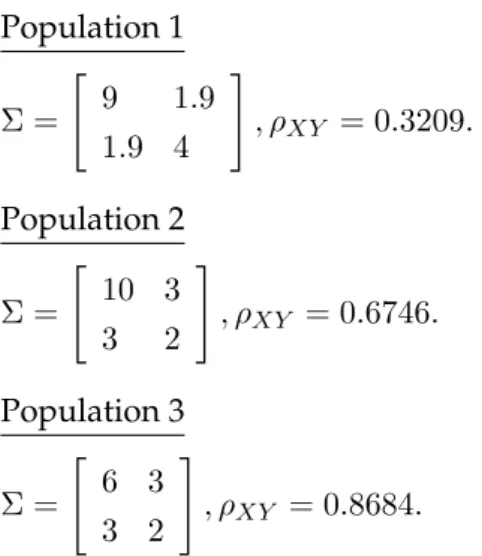
We considered 3 bivariate normal populations with different covariance matrices to represent the distribution of(Y, X). The scrambling variable Sis taken to be a normal distribution with mean equal to zero and standard deviation equal to 10% of the standard deviation ofX. The reported response is given byZ =Y +S.
All of the simulated populations have theoretical mean of[Y, X]asµ= [2,2]and co-variance matrices as given below.
Population 1
N = 1000
Σ =
"
9 1.9 1.9 4
#
, ρXY = 0.3167.
Population 2
N = 1000
Σ =
"
10 3 3 2
#
, ρXY = 0.6708.
Population 3
N = 1000
Σ =
"
6 3 3 2
#
, ρXY = 0.8660.
For each population we considered five sample sizes:n= 20,50,100,200and 300.
2.4. A Simulation Study
The RRT mean estimator should generally perform better than the ratio estimator because this is an unbiased estimator. Nevertheless, the ratio estimator produces fairly good results.
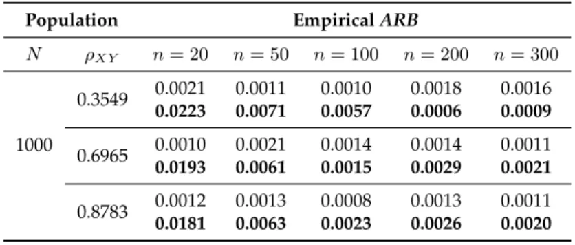
Table 2.1: EmpiricalARBfor RRT mean estimator and ratio estimator (bold).
Population EmpiricalARB
N ρXY n= 20 n= 50 n= 100 n= 200 n= 300
1000
0.3549 0.0021 0.0011 0.0010 0.0018 0.0016
0.0223 0.0071 0.0057 0.0006 0.0009
0.6965 0.0010 0.0021 0.0014 0.0014 0.0011
0.0193 0.0061 0.0015 0.0029 0.0021
0.8783 0.0012 0.0013 0.0008 0.0013 0.0011
0.0181 0.0063 0.0023 0.0026 0.0020
The theoreticalARBresults for the ratio estimator, correct up to first and second de-gree of approximation, are presented in Table2.2.
One can see that second order approximation as compared to first order approxima-tion does not result in major difference inARBeven for modest sample size ofn = 20
and50.
Table 2.2: TheoreticalARBfor ratio estimator based on1stand2ndorder (bold) approximation.
Population TheoreticalARB
N ρXY n= 20 n= 50 n= 100 n= 200 n= 300
1000
0.3549 0.0224 0.0087 0.0041 0.0018 0.0011
0.0258 0.0092 0.0042 0.0019 0.0011
0.6965 0.0155 0.0060 0.0029 0.0013 0.0007
0.0167 0.0062 0.0029 0.0013 0.0007
0.8783 0.0142 0.0055 0.0026 0.0012 0.0007
0.0153 0.0057 0.0026 0.0012 0.0007
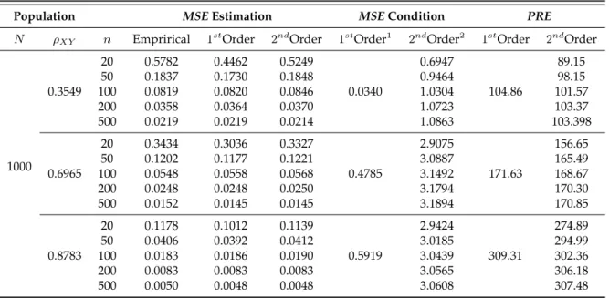
Table2.3below gives empirical and theoreticalMSE’sfor the ratio estimator based on both the first order and second order approximations. As we see from the table, there is hardly a difference between the two approximations even for small samples. Hence the Percent Relative Efficiency (PRE) is calculated based on first order of approximation only. We use the following expression to find thePREof ratio estimator as compared to the RRT mean estimator:
P RE = M SE(ˆµY)
M SE(ˆµR) ×
100.
2.5. Numerical Example
There are small differences betweenMSEvalues based on first and second order ap-proximation for smaller sample sizes (n=20 and 50) but theMSEvalues are very similar when the sample size is larger. We can also note that the ratio estimator gets more and more efficient as the coefficient of correlation betweenXandY increases. We can further note that for small correlation values, the ratio estimator may not be better than the RRT mean estimator, particularly so if sample size is small.
Table 2.3:MSEcorrect up to1stand2ndorder approximations and
PREfor the ratio estimator relative to the RRT mean estimator.
Population MSEEstimation MSECondition PRE
N ρXY n Emprirical 1stOrder 2ndOrder 1stOrder
1
2ndOrder2
1stOrder 2ndOrder
1000
0.3549
20 0.5782 0.4462 0.5249
0.0340
0.6947
104.86
89.15
50 0.1837 0.1730 0.1848 0.9464 98.15
100 0.0819 0.0820 0.0846 1.0304 101.57
200 0.0358 0.0364 0.0370 1.0723 103.37
500 0.0219 0.0219 0.0214 1.0863 103.398
0.6965
20 0.3434 0.3036 0.3327
0.4785
2.9075
171.63
156.65
50 0.1202 0.1177 0.1221 3.0887 165.49
100 0.0548 0.0558 0.0568 3.1492 168.67
200 0.0248 0.0248 0.0250 3.1794 170.30
500 0.0152 0.0145 0.0145 3.1894 170.85
0.8783
20 0.1178 0.1012 0.1139
0.5919
2.9424
309.31
274.89
50 0.0406 0.0392 0.0412 3.0185 294.99
100 0.0183 0.0186 0.0190 3.0439 302.36
200 0.0083 0.0083 0.0083 3.0565 306.18
500 0.0050 0.0048 0.0048 3.0608 307.48
1
MSEcomparison condition based on1storder approximation given in expression (2.9).
2
MSEcomparison condition based on2ndorder approximation given in expression (2.10).
2.5
Numerical Example
We now compare the RRT mean estimator and the ratio estimator using a real data set. The data come from a sample from the survey on Information and Communication Tech-nologies (ICT) usage in enterprises in 2009 with seat in Portugal (Smilhily and Storm, 2010). This survey intends to promote the development of the national statistical sys-tem in the information society and to contribute to a deeper knowledge about the usage of ICT by enterprises. The target population covers all industries with one and more persons employed in the sections of economic activity C (Manufacturing) to N (Admin-istrative and support service activities) and S (Other service activities), from NACE1Rev.
2 (Eurostat, 2008). The data are essentially collected using Electronic Data Interchange, applying direct connection between information systems at the respondent and the Na-tional Statistics Institute. For some enterprises the paper questionnaire is still used. The
1
2.5. Numerical Example
questions in the structural business surveys mainly deal with characteristics that can be found in the organisations’ annual reports and financial statements, such as employment, turnover and investment.
In our application the study variableY is the purchase orders in 2009, collected by the ICT survey in that year. This is typically a confidential variable for enterprises, only known from business surveys. The auxiliary variable X is the turnover of each enter-prise. This information can be easily obtained from enterprise records available in the public domain, as administrative information. In 2009 the population survey contained approximately278000enterprises and we know the value ofXfor all these enterprises. The purchase orders information was collected in the ICT survey and we have the val-ues ofY for 5090 enterprises (which answered this question in the ICT survey in 2009). For this study, these 5090enterprises are considered as our population. The scrambling variableSis taken to be a normal random variable with mean equal to zero and standard deviation equal to10%of the satandard deviation ofX, that isσS = 0.1σX. The reported response is given byZ =Y +S(the purchase order value plus a random quantity). The variablesY andXare strongly correlated so we can take advantage of this correla-tion by using the ratio estimator. In the next tables we present the results for the RRT mean estimator and for the ratio estimator for different sample sizes.
Population Characteristics:
N = 5090, ρXY = 0.9832
µX = 32.53, µY = 26.06, σX = 183.42, σY = 67.07(in millions of Euros) γX
1 = 31.54, γ1Y = 36.12, γ2X = 1481.08, γ2Y = 1839.13
where γ1 and γ2 are the coefficients of skewness andkurtosis, respectively. We use the
following samples sizes in our simulation study: n = 100,200,300,400,500,1000,1500
and2000.
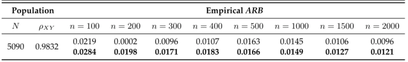
The empiricalARBvalues for both estimators, based on 5000 iterations, are given in Table 2.4. As expected, the bias decreases as the sample size increases, except for some random fluctuation. We expect the RRT mean estimator to perform better than the ratio estimator because this is an unbiased estimator, however, we don’t see major differences between the two for larger samples.
Table 2.4: EmpiricalARBfor the RRT mean estimator and the ratio estimator (bold).
Population EmpiricalARB
N ρXY n= 100 n= 200 n= 300 n= 400 n= 500 n= 1000 n= 1500 n= 2000
5090 0.9832 0.0219 0.0002 0.0096 0.0107 0.0163 0.0145 0.0106 0.0096
2.6. Transformed Ratio Estimators
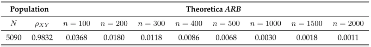
The theoretical ARB results for the ratio estimator, correct up to first degree of ap-proximation, are presented in Table2.5. We use only the first order approximations from here on since the first and second order approximations are very similar, as we have seen earlier.
Table 2.5: TheoreticalARBfor the RRT mean estimator and the ratio estimator.
Population TheoreticaARB
N ρXY n= 100 n= 200 n= 300 n= 400 n= 500 n= 1000 n= 1500 n= 2000
5090 0.9832 0.0368 0.0180 0.0118 0.0086 0.0068 0.0030 0.0018 0.0011
Table 2.6 presents the results for the empirical MSE estimates, the theoretical esti-mates, correct up to first degree of approximation and thePREof ratio estimator relative to the RRT mean estimator.
Table 2.6: MSE, corrected to1storder approximation, and
PREfor the ratio estimator related to the RRT mean estimator.
Population MSEEstimation
PRE
N ρXY n Empirical Theoretical
5090 0.9832
100 12.8924 15.2630
2286.36 200 6.4608 7.4786
300 4.4498 4.8838 400 3.5279 3.5864 500 2.7380 2.8079 1000 1.4117 1.2510 1500 0.8805 0.7321 2000 0.6033 0.4726
Clearly the ratio estimator performs better than the RRT mean estimator for the real data also. The effect of sample size on thePREcalculation is neutralized when first order approximation is used, as can be seen from Equations (2.2) and (2.8).
2.6
Transformed Ratio Estimators
Now consider the transformed ratio estimator:
ˆ
µT R= ¯z
cX¯ +d cx¯+d
, (2.11)
2.6. Transformed Ratio Estimators
We can rewrite (2.11) using relative error terms in the form
ˆ
µT R= ¯z(1 +δz) (1 +ηδx)−1, (2.12)
whereη = cX¯
cX¯+d.
Expanding (2.12), theBias, correct up to first order of approximation, is given by
Bias(1)(ˆµT R)∼=
1−f n
¯
Y{η2Cx2−ηρyxCyCx}. (2.13)
By (2.6) and (2.13)Bias(1)(ˆµT R)< Bias(1)(ˆµR)if
(η−1)
ρyx−
(η+ 1)Cx Cy
>0. (2.14)
SimilarlyMSEofµˆT R, to first order of approximation, is given by
M SE(1)(ˆµT R)∼=
1−f n
¯
Y2 Cy2+η2Cx2−2ηρyxCyCx
. (2.15)
By (2.8) and (2.15)M SE(1)(ˆµT R)< M SE(1)(ˆµR)if
(η−1)
ρyx−
(η+ 1)Cx
2Cy
>0. (2.16)
Now we conduct a simulation study with particular focus on the comparison between the ratio estimatorµˆRand the transformed ratio estimatorµˆT R. We considered the same three bivariate normal populations as in the previous simulation study (Section2.4).
The scrambling variableS is taken to be a normal random variable with mean equal to zero and the standard deviation equal to 10% of the standard deviation of X. The reported response is given byZ = Y +S. To compare these estimators, we present the results for the RRT mean estimator (ˆµY), the ratio estimator(ˆµR) and for transformed ratio estimatorµˆT Ri(i= 1,2,3,4)with four different combinations of parameterscandd:
1. µˆT R1 = ¯z
cX¯ +d cx¯+d
,
wherec= 1andd=coefficient ofskewness;
2. µˆT R2 = ¯z
cX¯ +d cx¯+d
,
wherec= 1andd=coefficient ofkurtosis;
3. µˆT R3 = ¯z
cX¯ +d cx¯+d
,
2.6. Transformed Ratio Estimators
4. µˆT R4 = ¯z
cX¯ +d cx¯+d
,
wherec=coefficient ofkurtosisandd=coefficient ofskewness.
The empiricalARBvalues for these six estimators are given in Table2.7.
Table 2.7: EmpiricalARBfor the RRT mean estimator, the ratio estimator and for the transformed ratio estimators.
Population EmpiricalARB
N ρXY n µˆY µˆR µˆT R1 µˆT R2 µˆT R3 µˆT R4
1000
0.3209
20 0.0002 0.0337 0.0435 0.0006 0.0026 0.0366 50 0.0007 0.0118 0.0146 0.0002 0.0019 0.0126 100 0.0003 0.0052 0.0065 0.0000 0.0009 0.0056 150 0.0000 0.0032 0.0040 0.0001 0.0003 0.0035 200 0.0012 0.0025 0.0030 0.0008 0.0016 0.0027 300 0.0020 0.0041 0.0045 0.0023 0.0021 0.0043
0.6746
20 0.0011 0.0122 0.0113 0.0111 0.0018 0.0119 50 0.0004 0.0042 0.0038 0.0037 0.0015 0.0041 100 0.0001 0.0022 0.0021 0.0021 0.0005 0.0022 150 0.0005 0.0016 0.0015 0.0016 0.0002 0.0016 200 0.0010 0.0005 0.0005 0.0001 0.0013 0.0005 300 0.0015 0.0013 0.0014 0.0011 0.0016 0.0014
0.8684
20 0.0006 0.0120 0.0115 0.0108 0.0013 0.0119 50 0.0005 0.0041 0.0039 0.0036 0.0012 0.0040 100 0.0001 0.0018 0.0017 0.0017 0.0005 0.0018 150 0.0002 0.0010 0.0010 0.0012 0.0001 0.0010 200 0.0009 0.0004 0.0004 0.0001 0.0011 0.0004 300 0.0014 0.0010 0.0011 0.0010 0.0015 0.0010
2.6. Transformed Ratio Estimators
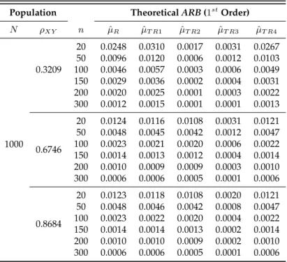
Table 2.8: TheoreticalARBto1storder approximation for the RRT mean estimator, the ratio estimator and
for the transformed ratio estimators.
Population TheoreticalARB(1stOrder) N ρXY n µˆR µˆT R1 µˆT R2 µˆT R3 µˆT R4
1000
0.3209
20 0.0248 0.0310 0.0017 0.0031 0.0267 50 0.0096 0.0120 0.0006 0.0012 0.0103 100 0.0046 0.0057 0.0003 0.0006 0.0049 150 0.0029 0.0036 0.0002 0.0004 0.0031 200 0.0020 0.0025 0.0001 0.0003 0.0022 300 0.0012 0.0015 0.0001 0.0001 0.0013
0.6746
20 0.0124 0.0116 0.0108 0.0031 0.0121 50 0.0048 0.0045 0.0042 0.0012 0.0047 100 0.0023 0.0021 0.0020 0.0006 0.0022 150 0.0014 0.0013 0.0012 0.0004 0.0014 200 0.0010 0.0009 0.0009 0.0003 0.0010 300 0.0006 0.0006 0.0005 0.0001 0.0006
0.8684
20 0.0123 0.0118 0.0108 0.0020 0.0121 50 0.0048 0.0046 0.0042 0.0008 0.0047 100 0.0023 0.0022 0.0020 0.0004 0.0022 150 0.0014 0.0014 0.0013 0.0002 0.0014 200 0.0010 0.0010 0.0009 0.0002 0.0010 300 0.0006 0.0006 0.0005 0.0001 0.0006
2.6. Transformed Ratio Estimators
Table 2.9: EmpiricalMSEand theoretical (bold)MSEto1storder of approximation for the RRT mean
esti-mator, the ratio estimator and for the transformed ratio estimators.
Population MSE
N ρXY n µˆR µˆT R1 µˆT R2 µˆT R3 µˆT R4
1000
0.3209
20 0.5799 0.6584 0.4097 0.4686 0.6010
0.4496 0.4672 0.3994 0.4663 0.4548
50 0.1881 0.2000 0.1546 0.1793 0.1915
0.1743 0.1811 0.1549 0.1808 0.1763
100 0.0872 0.0914 0.0750 0.0875 0.0884
0.0826 0.0858 0.0734 0.0857 0.0835
150 0.0546 0.0571 0.0475 0.0551 0.0554
0.0520 0.0540 0.0462 0.0539 0.0526
200 0.0395 0.0412 0.0343 0.0394 0.0400
0.0367 0.0381 0.0326 0.0381 0.0371
300 0.0223 0.0232 0.0196 0.0227 0.0225
0.0214 0.0222 0.0190 0.0222 0.0217
0.6746
20 0.3226 0.3197 0.3956 0.5167 0.3216
0.2939 0.2884 0.3885 0.5162 0.2961
50 0.1165 0.1148 0.1497 0.1979 0.1159
0.1140 0.1118 0.1507 0.2002 0.1132
100 0.0558 0.0548 0.0728 0.0967 0.0554
0.0540 0.0530 0.0714 0.0948 0.0536
150 0.0352 0.0346 0.0460 0.0608 0.0350
0.0340 0.0333 0.0449 0.0597 0.0338
200 0.0254 0.0250 0.0330 0.0434 0.0253
0.0240 0.0235 0.0317 0.0421 0.0238
300 0.0145 0.0142 0.0189 0.0250 0.0144
0.0140 0.0137 0.0185 0.0246 0.0139
0.8684
20 0.1117 0.1083 0.1973 0.3119 0.1106
0.0984 0.0947 0.1920 0.3113 0.0971
50 0.0396 0.0382 0.0743 0.1195 0.0391
0.0381 0.0367 0.0744 0.1207 0.0377
100 0.0188 0.0181 0.0361 0.0584 0.0186
0.0181 0.0174 0.0353 0.0572 0.0178
150 0.0118 0.0114 0.0228 0.0367 0.0117
0.0114 0.0110 0.0222 0.0360 0.0112
200 0.0086 0.0083 0.0164 0.0263 0.0085
0.0080 0.0077 0.0157 0.0254 0.0079
300 0.0049 0.0047 0.0094 0.0151 0.0048
0.0047 0.0045 0.0091 0.0148 0.0046
Table2.10gives thePREof various transformed ratio estimators relative to the ratio estimator based on first order approximation.
2.7. Conclusions
Table 2.10: PRE for the transformed ratio estimator related to the ratio estimator based on 1st order of
approximation.
Population PRE(1stOrder) N ρXY µˆT R1 µˆT R2 µˆT R3 µˆT R4
1000
0.3209 96.24 112.56 96.41 98.86 0.6746 101.93 75.65 56.94 100.64 0.8684 103.87 51.24 31.60 101.28
Note that the transformed ratio estimator performs better than the ratio estimator when the condition in (2.16) is satisfied.
Table 2.11: Calculations for the expression in (2.16).
Population Condition(MSE-1st
Order)
N ρXY µˆT R1 µˆT R2 µˆT R3 µˆT R4
1000
0.3209 -0.0299 0.0855 -0.0285 -0.0088 0.6746 0.0127 -0.2160 -0.5074 0.0043 0.8684 0.0108 -0.2751 -0.6259 0.0037
2.7
Conclusions
We can observe from this study that the estimation of the mean of a sensitive variable can be improved by using a non-sensitive auxiliary variable. The ratio estimators, in spite of being biased, can have much betterPREas compared to the RRT mean estima-tor. Our simulation study and the numerical example show that this improvement can be quite substantial if the correlation between the study variable and the auxiliary vari-able is high. We also note that there is hardly any difference in theBias or MSEof the proposed estimator when using first or second order approximation. It is further noticed that the transformed ratio estimators produce very minimal gain over the ordinary ratio estimator.
References
CHANDRA, P. & SINGH, H. P. 2005. A family of estimators for population variance using knowledge of kurtosis of an auxiliary variable in sample surveys.Statistics in Tran-sition, 7(1), 27-34.
EICHHORN, B. H. & HAYRE, L. S. 1983. Scrambled randomized response methods for obtaining sensitive quantitative data. Journal of Statistical Planning and Inference, 7, 307-316.
References
European Community. Official Publications of the European Communities, 112-285 and 306-311.
GUPTA, S. N., GUPTA, B. C. & SINGH, S. 2002. Estimation of sensitivity level of personal interview survey questions.Journal of Statistical Planning and Inference, 100, 239-247. GUPTA, S. & SHABBIR, J. 2004. Sensitivity estimation for personal interview survey questions.Statistica, 64, 643-653.
GUPTA, S., SHABBIR, J. & SEHRA, S. 2010. Mean and sensitivity estimation in optional randomized response models. Journal of Statistical Planning and Inference, 140(10), 2870-2874.
KADILAR, C. & CINGI, H. 2006. Improvement in estimating the population mean in simple random sampling.Applied Mathematics Letters, 19(1), 75-79.
KOYUNCU, N. & KADILAR, C. 2009. Efficient estimators for the population mean, Hacettepe Journal of Mathematics and Statistics, 38(2), 217-225.
KULKARNI, S. P. 1977. A note on modified ratio estimator using transformation,Journal of the Indian Society of Agricultural Statistics, 30(2), 125-128.
SAHA, A. 2008. A randomized response technique for quantitative data under unequal probability sampling.Journal of statistical Theory and Practice, 2(4), 589-596.
SHABBIR, J. & GUPTA, S. 2010. Estimation of the finite population mean in two-phase sampling when auxiliary variables are attribute,Hacettepe Journal of Mathematics and Statis-tics, 39(1), 121-129.
SINGH, J., PANDAY, B. N. & HIRANO, K. 1973. On the utilization of a known coefficient of kurtosis in the estimation procedure of variance. Annals of the Institute of Statistical Mathematics, 25, 51-55.
SINGH, H. P. & VISHWAKARMA, G. 2008. Some families of estimators of variance of stratified random sample mean using auxiliary information. Journal of Statistical Theory and Practice, 2(1), 21-43.
SISODIA, B. V. S. & DWIDEDI, V. K. 1981. A modified ratio estimator using coefficient of variation of auxiliary variable. Journal of the Indian Society of Agricultural Statistics, 33, 13-18.
SMILHILY, M. & STORM, H. 2010. ICT usage in enterprises - 2009,Eurostat Publications, Issue 1.
SUKHATME, P.V. & SUKHATME, B.V. 1984. Sampling theory of surveys with applications,
3rdEd., Ames, Iowa, Iowa State University Press.
References
using auxiliary information. Hacettepe Journal of Mathematics and Statistics, 37(2), 177-184. UPADHYAYA, L. N. & SINGH, H. P. 1999. Use of transformed auxiliary variable in esti-mating the finite population mean.Biometrical Journal, 41(5), 627-636.
Appendix A - R Routines
Appendix A - R Routines
Listing 2.1: R Code for Simulation Study of Proposed Estimator in Chapter 2
1
2 proj1 <- function(N,sigma,mu) 3 {
4 set.seed(100)
5 #Generation of a bivariate normal population 6 data_yx <- mvrnorm(N, mu, sigma)
7
8 #Study variable 9 Y <- data_yx[,1]
10 #Auxiliary variable, correlated with Y
11 X <- data_yx[,2] 12
13 #Coefficient of correlation between Y and X
14 Ro_YX <- cor(Y,X) 15
16 #Scrambling variable independent of Y and X, with mean=0 17 S <- rnorm(N,mean=0,sd=0.1*sd(X))
18 #Scrambled response 19 Z <- Y+S
20
21 #Coefficient of correlation between Z and X 22 Ro_ZX <- Ro_YX/sqrt(1+(var(S)/var(Y))) 23
24 #population
25 univ <- data.frame(cbind(Y=Y,S=S,Z=Z,X=X,NRAND=runif(N))) 26 univ <- univ[order(univ$NRAND),]
27
28 #Mean of Y
29 my <- mean(univ$Y) 30 mz <- mean(univ$Z) 31 mx <- mean(univ$X) 32 ms <- mean(univ$S) 33
34 #Sample dimension
35 dim_samp <- c(20,50,100,200,300) 36
37 res <- NULL
38 for (i in 1:length(dim_samp)) 39 {
40 #sample dimension 41 n <- dim_samp[i] 42 #sample
43 samp <- univ[1:n,] 44 #sampling rate
Appendix A - R Routines
47 #estimators
48 est1 <- mean(samp$Z)
49 est2 <- mean(samp$Z)*(mean(univ$X)/mean(samp$X)) 50
51 #Ratio
52 R <- mean(univ$X)/mean(samp$X) 53
54 #Mean Square Error of 1st estimator 55 mse1 <- ((1-f)/n)*var(univ$Z)
56
57 #Coefficient of variation
58 c_x <- sd(univ$X)/mx 59 c_y <- sd(univ$Y)/my 60 c2_x <- c_x^2
61 c2_y <- c_y^2
62 c2_z <- c2_y+(var(univ$S)/(my^2)) 63 c_z <- sqrt(c2_z)
64
65 #Bias of ratio estimator - 1st degree approximation 66 bias2i <- ((1-f)/n)*my*(c2_x-Ro_ZX*c_z*c_x)
67 #Bias of ratio estimator - 2nd degree approximation 68 bias2ii <- bias2i*(1+((1-f)/n)*3*c2_x)
69
70 #Mean Square Error of ratio estimator - 1st degree approximation 71 mse2i <- ((1-f)/n)*(my^2)*(c2_z+c2_x-2*Ro_ZX*c_z*c_x)
72 #Mean Square Error of ratio estimator - 2nd degree approximation
73 mse2ii <- mse2i+3*(my^2)*(((1-f)/n)^2)*c2_x*((1+2*(Ro_ZX^2))*c2_z 74 +3*c2_x-6*Ro_ZX*c_z*c_x)
75
76 aux_bias <- (c_x-Ro_ZX*c_z) 77
78 aux_mse1 <- (Ro_ZX-(1/2)*(c_x/c_z))
79 aux_mse2 <- 2*Ro_ZX*(c_z/c_x)-3*((1-f)/n)*((1+2*(Ro_ZX^2))*c2_z 80 +3*c2_x-6*Ro_ZX*c_z*c_x)
81
82 emp <- NULL 83
84 #Empirical results
85 #Simulation of 5000 replicas of estimates 86 ...
87
88 #Results
89 res <- rbind(res,c(N,n,Ro_YX,Ro_ZX,R,my,mz,ms, 90 med_est1,med_est2,bias2i,bias2ii,emp_mse1,mse1, 91 emp_mse2,mse2i,mse2ii,aux_bias,aux_mse1,aux_mse2)) 92 }
93 colnames(res) <- c("N","n","RhoXY","RhoZX","R","mY","mZ","mS", 94 "Est1","Est2","BIAS2I","BIAS2II","EMP_MSE1","MSE1",
Appendix A - R Routines
97 } 98
99 #Package for generation 100 require(MASS)
101 N<-1000 102 #Parameters
103 sigma1 <- matrix(c(9,1.9,1.9,4),2,2) 104 sigma2 <- matrix(c(10,3,3,2),2,2) 105 sigma3 <- matrix(c(6,3,3,2),2,2) 106 mu <- c(2,2)
107
108 res <- NULL
109 for (i in 1:length(N)) 110 {
111 res <- rbind(res,proj1(N[i],sigma1,mu)) 112 res <- rbind(res,proj1(N[i],sigma2,mu)) 113 res <- rbind(res,proj1(N[i],sigma3,mu)) 114 }
Appendix A - R Routines
Listing 2.2: R Code for Simulation Study of Transformed Ratio Estimators in Chapter 2
1
2 mykurtosis <- function(x) 3 {
4 m4 <- mean((x-mean(x))^4) 5 kurt <- m4/(sd(x)^4) 6 return(kurt)
7 }
8 myskewness <- function(x) 9 {
10 m3 <- mean((x-mean(x))^3)
11 skew <- m3/(sd(x)^3) 12 return(skew)
13 }
14 proj1_transf <- function(N,sigma,mu) 15 {
16
17 #Generation of a bivariate normal population 18 data_yx <- mvrnorm(N, mu, sigma)
19
20 #Study variable 21 Y <- data_yx[,1]
22 #Auxiliary variable, correlated with Y 23 X <- data_yx[,2]
24
25 #Coefficient of correlation between Y and X 26 Ro_YX <- cor(Y,X)
27
28 #Scrambling variable independent of Y and X, with mean=0
29 S <- rnorm(N,mean=0,sd=0.1*sd(X)) 30 #Scrambled response
31 Z <- Y+S 32
33 #Coefficient of correlation between Z and X 34 Ro_ZX <- Ro_YX/sqrt(1+(var(S)/var(Y))) 35
36 #population
37 univ <- data.frame(cbind(Y=Y,S=S,Z=Z,X=X,NRAND=runif(N))) 38 univ <- univ[order(univ$NRAND),]
39
40 #Mean of Y
41 my <- mean(univ$Y) 42 mz <- mean(univ$Z) 43 mx <- mean(univ$X) 44
45 #Samples dimension
Appendix A - R Routines
48 res <- NULL
49 for (i in 1:length(dim_samp)) 50 {
51 #sample dimension 52 n <- dim_samp[i] 53 #sample
54 samp <- univ[1:n,] 55 #sampling rate 56 f <- n/N 57
58 #Ratio
59 R <- mean(univ$X)/mean(samp$X) 60
61 #Ordinary meam 62 est1 <- mean(samp$Z) 63 #Ratio estimator
64 est2 <- mean(samp$Z)*(mean(univ$X)/mean(samp$X)) 65
66 #Coefficient of variation 67 c_x <- sd(univ$X)/mx 68 c_y <- sd(univ$Y)/my 69 c2_x <- c_x^2
70 c2_y <- c_y^2
71 c2_z <- c2_y+(var(univ$S)/(my^2)) 72 c_z <- sqrt(c2_z)
73
74 #Bias of ratio estimator - 1st degree approximation
75 bias2i <- ((1-f)/n)*my*(c2_x-Ro_ZX*c_z*c_x)
76 #Bias of ratio estimator - 2nd degree approximation
77 bias2ii <- bias2i*(1+((1-f)/n)*3*c2_x) 78
79 #Mean Square Error of 1st estimator (ordinal mean) 80 mse1 <- ((1-f)/n)*(var(univ$Y)+var(univ$S))
81
82 #Mean Square Error of ratio estimator - 1st degree approximation 83 mse2i <- ((1-f)/n)*(my^2)*(c2_z+c2_x-2*Ro_ZX*c_z*c_x)
84 #Mean Square Error of ratio estimator - 2nd degree approximation 85 mse2ii <- mse2i+3*(my^2)*(((1-f)/n)^2)*c2_x*((1+2*(Ro_ZX^2))*c2_z
86 +3*c2_x-6*Ro_ZX*c_z*c_x)
87
88 nu <- 1
89 aux_m <- c2_x-2*Ro_ZX*c_z*c_x
90
91 s <- myskewness(univ$X) 92 k <- mykurtosis(univ$X) 93
94 vc <- c(1,1,1,s,k) 95 vd <- c(s,k,Ro_YX,k,s) 96
Appendix A - R Routines
98
99 for (i in 1:length(vc)) 100 {
101 nu <- (vc[i]*mean(univ$X))/(vc[i]*mean(univ$X)+vd[i]) 102 vnu <- c(vnu,nu)
103
104 aux_bias1 <- (nu-1)*(Ro_ZX-(nu+1)*c_x/c_z)
105 aux_mse1 <- (nu-1)*(Ro_ZX-(nu+1)*c_x/(2*c_z))
106
107 vb1 <- c(vb1,aux_bias1) 108 vm1 <- c(vm1,aux_mse1) 109
110 #Transformed ratio estimator
111 est3 <- c(est3,mean(samp$Z)*(vc[i]*mean(univ$X)+vd[i])
112 /(vc[i]*mean(samp$X)+vd[i]))
113
114 #Mean Square Error of transformed ratio estimator 115 #1st degree approximation
116 mse3i <- c(mse3i,((1-f)/n)*(my^2)*(c2_z+(nu^2)*c2_x-2*nu*Ro_ZX*c_z*c_x)) 117
118 #Mean Square Error of transformed ratio estimator 119 #1st degree approximation
120 mse3ii <- c(mse3ii,mse3i[i]+3*(my^2)
121 *(((1-f)/n)^2)*c2_x*((nu^2)*(1+2*(Ro_ZX^2))
122 *c2_z+3*(nu^4)*c2_x-6*(nu^3)*Ro_ZX*c_z*c_x))
123
124 #Bias of transformated ratio estimator - 1st degree approximation
125 bias3i <- c(bias3i,((1-f)/n)*my*((nu^2)*c2_x-nu*Ro_ZX*c_z*c_x)) 126 #Bias of transformated ratio estimator - 2nd degree approximation
127 bias3ii <- c(bias3ii,bias3i[i]
128 +(((1-f)/n)^2)*3*my*((nu^4)*(c2_x^2)-(nu^3)
129 *Ro_ZX*c_z*(c_x^3)))
130 } 131
132 #Empirical results
133 #Simulation of 5000 replicas of estimates 134 ...
135
136 #Results
137 res <- rbind(res,c(N,n,Ro_YX,Ro_ZX,R,my,med_est1,med_est2,
138 med_est3,
139 bias2i,bias2ii,
140 bias3i,
141 bias3ii,
142 emp_mse1,mse1,emp_mse2,mse2i,mse2ii,
143 emp_mse3,
144 mse3i,
145 mse3ii,
146 vnu,
Appendix A - R Routines
148 vm1))
149 }
150 colnames(res) <- c("N","n","RhoXY","RhoZX","R","mY","Est1","Est2", 151 paste("Est3_",1:length(vc),sep=""),
152 "BIAS2I","BIAS2II",
153 paste("BIAS3I_",1:length(vc),sep=""), 154 paste("BIAS3II_",1:length(vc),sep=""),
155 "EMP_MSE1","MSE1","EMP_MSE2","MSE2I","MSE2II", 156 paste("EMP_MSE3_",1:length(vc),sep=""),
157 paste("MSE3I_",1:length(vc),sep=""), 158 paste("MSE3II_",1:length(vc),sep=""), 159 paste("NU_",1:length(vc),sep=""),
160 paste("AUX3_BIAS1_",1:length(vc),sep=""), 161 paste("AUX3_MSE1_",1:length(vc),sep="")) 162 return(res)
163 }
164 #Package for generation 165 require(MASS)
166 N <- 1000 167
168 #Parameters
169 sigma1 <- matrix(c(9,1.9,1.9,4),2,2) 170 sigma2 <- matrix(c(10,3,3,2),2,2) 171 sigma3 <- matrix(c(6,3,3,2),2,2) 172 mu <- c(2,2)
173
174 res <- NULL
175 for (i in 1:length(N)) 176 {
177 res <- rbind(res,proj1_transf(N[i],sigma1,mu)) 178 res <- rbind(res,proj1_transf(N[i],sigma2,mu)) 179 res <- rbind(res,proj1_transf(N[i],sigma3,mu)) 180 }
Appendix A - R Routines
Listing 2.3: R Code for Numerical Example of Proposed Estimator in Chapter 2
1
2 proj1_real <- function(Y,X,N) 3 {
4
5 #Coefficient of correlation between Y and X 6 Ro_YX <- cor(Y,X)
7
8 #Scrambling variable independent of Y and X, with mean=0 9 S <- rnorm(N,mean=0,sd=sd(X)*0.1)
10 #Scrambled response
11 Z <- Y+S 12
13 #Coefficient of correlation between Z and X
14 Ro_ZX <- Ro_YX/sqrt(1+(var(S)/var(Y))) 15
16 #population
17 univ <- data.frame(cbind(Y=Y,S=S,Z=Z,X=X,NRAND=runif(N))) 18 univ <- univ[order(univ$NRAND),]
19
20 #Mean of Y
21 my <- mean(univ$Y) 22 mz <- mean(univ$Z) 23 mx <- mean(univ$X) 24
25 #Samples dimension
26 dim_samp <- c(100,200,300,400,500,1000,1500,2000) 27
28 res <- NULL
29 for (i in 1:length(dim_samp)) 30 {
31 #sample dimension
32 n <- dim_samp[i] 33 #sample
34 samp <- univ[1:n,] 35 #Sampling rate 36 f <- n/N 37
38 #estimators
39 est1 <- mean(samp$Z)
40 est2 <- mean(samp$Z)*(mean(univ$X)/mean(samp$X))
41
42 #Ratio
43 R <- mean(univ$X)/mean(samp$X) 44
45 #Mean Square Error of 1st estimator