Study of nuclear reactions relevant for Astrophysics by Micro-AMS

(1)

Hélio Fernandes Luis

Mestre

Study of nuclear reactions relevant for

Astrophysics by Micro-AMS

Dissertação para obtenção do Grau de Doutor em

Física

Orientador: Adelaide Pedro Jesus, Professora catedrática,

FCT/UNL

Júri:

Presidente: Dr. Maria Paula Pires dos Santos

Diogo

Arguentes: Dr. Rui Coelho Silva

Dr. Orlando Teodoro

Vogais: Dr. João Cruz

Dr. Daniel Redondo

(2)

(3)

Study of nuclear reactions relevant for Astrophysics by Micro-AMS

(4)

(5)

Acknowledgements

I would like to thank Prof. Dr. Adelaide Jesus for the orientation of this thesis's work. I would also like to thank Dr. Soey Sie, Dr. Nuno Franco, Eng. Jorge Rocha, Dr. Eduardo Alves, Dr. Micaela Fonseca, Dr. João Cruz, Dr. Orlando Teodoro, Me. Cátia Santos, Me. Hugo Santos, Dr. Rui Coelho, Dr. Daniel Redondo, Eng. Paulo Velho, Dr. Carlos Cruz, , Me. Joana Lancastre and Me. Catarina Ramos for all the help they provided.

(6)

(7)

Resumo

Esta tese tem como base a aplicação da técnica de Micro-AMS (Espectrometria de massa com acelerador usando micro-feixe) ao estudo de reações nucleares relevantes para a Astrofísica,

nomeadamente através do estudo de reações envolvendo o radioisótopo 36_Cl.

A etapa inicial do trabalho prendeu-se com a instalação, teste e otimização do sistema de Micro-AMS que se encontra no laboratório de feixe de iões do CTN-IST. Na fase de testes foram medidos vários isótopos, nomeadamente isótopos de chumbo e platina, que revelaram o potencial desta técnica para aplicações em áreas tão diversas como a Ciência dos Materiais ou a Arqueologia. Após esta fase, deu-se o

inicio do trabalho com o 36_Cl.

O radioisótopo 36_{Cl é um dos isótopos de tempo de vida média curta (assim chamados por a sua}

vida média ser curta quando comparada com a idade da terra) cujas abundâncias no sistema solar primitivo poderão ajudar a esclarecer o seu processo de formação. Existem dois modelos geralmente

aceites para a produção deste radionuclido; é originário de ejecta de supernovas vizinhas (onde o 36_{Cl foi}

provavelmente produzido no processo s através da irradiação neutrónica de 35_{Cl) e/ou foi produzido}

através da irradiação in-situ de pó nebular por partículas energéticas (principalmente p, a, 3_{He - modelo de}

irradiação X-Wind).

O objectivo do presente trabalho foi a medição da secção eficaz da reação nuclear 35_Cl(n,_γ₎36_{Cl, que}

abriu a possibilidade da medição futura das secções eficazes das reações nucleares 37_Cl(p,d)36_Cl

e35_Cl(d,p)36_{Cl. Esta medição foi efectuada através da determinação da quantidade de}36_{Cl em amostras de}

AgCl, utilizando a referida técnica e tirando partido da sua alta sensibilidade para medições de cloro. Para tal, o sistema de Micro-AMS do CTN-IST teve que ser optimizado para medições de cloro uma vez que esta é a primeira vez que este tipo de medições foi executada (AMS com micro-feixe).

Esta tese apresenta os resultados destes desenvolvimentos que foram feitos comparando amostras de AgCl irradiadas no Reactor Nacional Português com amostras padrão produzidas através da diluição do material de referência NIST SRM 4943. Após a obtenção destes resultados, a secção eficaz da reacção

35

Cl(n,γ)36

Cl foi calculada.

Palavras-chave: Micro-AMS, 36_{Cl, secção eficaz, reação nuclear, Astrofísica, formação do}

(8)

(9)

Abstract

This work of this thesis was dedicated to the application of the Micro-AMS (Accelerator Mass spectrometry with micro-beam) to the study of nuclear reactions relevant to Astrophysics, namely reactions involving the radioisotope 36_Cl.

Before this could be done, the system had to be installed, tested and optimized. During the installation and testing phase, several isotopes were measured, principally lead and platinum isotopes, which served to show the potential of this technique for applications to Material science and archeology. After this initial stage, the work with 36_{Cl began.}

36_{Cl is one of several short to medium lived isotopes (as compared to the earth age) whose}

abundances in the earlier solar system may help to clarify its formation process. There are two generally accepted possible models for the production of this radionuclide: it originated from the ejecta of a nearby supernova (where 36_{Cl was most probably produced via the s-process by neutron}

irradiation of 35_{Cl) and/or it was produced by in-situ irradiation of nebular dust by energetic particles}

(mostly, p, a, 3_{He -X-wind irradiation model).}

The objective of the present work was to measure the cross section of the 35_Cl(n,_γ₎36_{Cl nuclear}

reaction which opened the possibility to the future study of the 37_Cl(p,d)36_{Cl and}35_Cl(d,p)36_{Cl nuclear}

reactions, by measuring the 36_{Cl content of AgCl samples with Micro-AMS, taking advantage of the}

very low detection limits of this technique for chlorine measurements.

For that, the micro-AMS system of the CTN-IST laboratory had to be optimized for chlorine measurements, as to our knowledge this type of measurements had never been performed in such a system (AMS with micro-beam).

This thesis presents the results of these developments, namely the tests in terms of precision and reproducibility that were done by comparing AgCl blanks irradiated at the Portuguese National Reactor with standards produced by the dilution of the NIST SRM 4943 standard material. With these results the cross section of the 37_Cl(n,_γ₎36_{Cl was calculated}.

Keywords: Micro-AMS, 36_{Cl, cross section, nuclear reaction, Astrophysics, solar system}

(10)

(11)

List of symbols

A activity

B magnetic field

! capacitance

c velocity of light

c(A) fractional concentration of element A

d distance

E energy

electrostatic field

! frequency

centripetal force

h amount of target material gw wescott factor

G gravitational constant Gres self-protection factor

L length

M mass

m mass

N number of nuclides NA Avogadro constant

n(A) concentration of element A ntot number of atoms

P attenuation factor

q charge

r radius

S linear stopping power SA,B separation factor

S1,M sputter rate

(12)

tirr irradiation time

U0 amplitude of AC signal

U surface binding energy

v velocity

V voltage

Z Atomic number

ξ electrostatic field

! angle

αq(P) Probability for ionization

φ neutron flux

σ cross-section

θX Natural abundance of isotope X

!_! Individual uncertainty

!_! real neutron flux

Y yield

Ytot total sputtering yield

ω angular frequency

r(AN₎ _{relative abundance of isotope}_AN

ntot number of target atoms/cm3

I electrical current

!! ! secondary current of a molecule P=ANBjMCk

(13)

!! isotopic ratio

THEq(AN) transmission of AN in charge state q through the HE spectometer

!_!"! ! transmission of P through LE mass spectometer

T half life

ε detector efficiency

!"#

!!

! _{relative sensitivity factor}

!! electron affinity

(14)

(15)

List of Figures

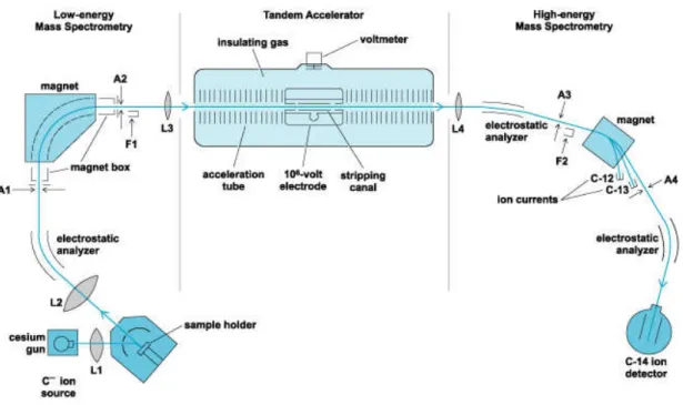
Figure 2.1: General scheme of a standard AMS beam line, using the example of 14_{C. F means}

Faraday cup. A means slits. L means focusing device. ___________________________________ 32

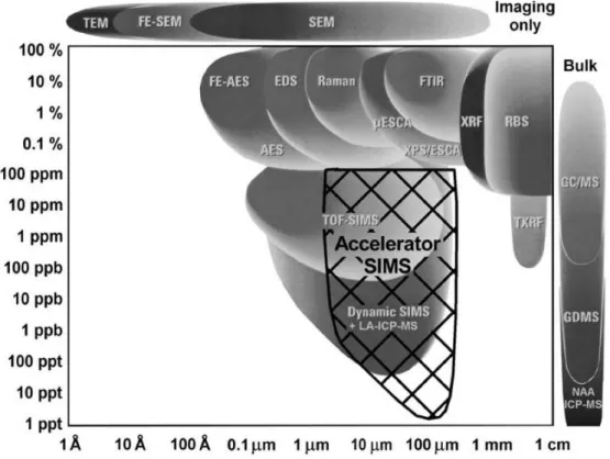
Figure 2.2: Atomic Force Microscopy (AFM), Scanning Electron Microscopy (SEM), Field Emission Scanning Electron Microscopy (FE-SEM), Transmission Electron Microscopy (TEM), Auger Electron Spectrometry (AES), Focussed Electron Beam Auger Electron Spectrometry (FE- AES), Energy Dispersive X-ray Spectrometry (EDS), µ-Raman Spectroscopy (Raman), X-Ray Photoelectron Spectroscopy (XPS), Electron Spectroscopy for Chemical Analysis (ESCA), Fourier Transform Infrared Spectrometry (FTIR), X-Ray Fluorescence (XRF), Rutherford Backscattering Spectrometry (RBS), Total Reflection X-Ray Fluorescence (TXRF), Time-of-Flight Secondary Ion Mass Spectrometry (TOF-SIMS), Secondary Ion Mass Spectrometry (Dynamic-SIMS), Inductively Coupled Plasma Mass Spectrometry (ICP-MS), Laser Ablation ICP-MS (LA-ICP-MS), Gas Chromatography/Mass Spectrometry (GCMS), Glow Discharge Mass Spectrometry (GDMS), Neutron Activation Analysis (NAA) _____________________________ 41

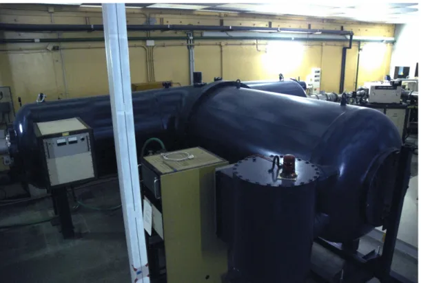
Figure 3.1: 3 MV tandem accelerator at LATR/CTN-ITN. ________________________________ 45

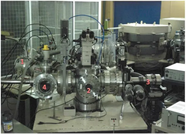
Figure 3.2: Micro-AMS chamber at LATR/CTN-ITN. In this image it is visible the ion source on the left side behind the vacuum lock system, the microscope on top of the chamber. The smaller circular glass window on the main chamber allows the operator to view the target holder. ___ 46

Figure 3.3: b) Scheme of the interior of the modified hiconex ion source. __________________ 47

Figure 3.4: General scheme of the target chamber. _____________________________________ 49

Figure 3.5: General view of the injection system at LATR/CTN-ITN. _____________________ 51

Figure 3.6: General scheme of the injection system, with all its different elements. ___________ 53

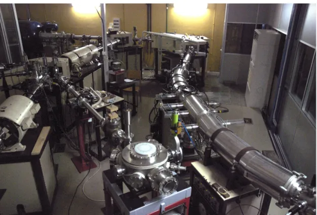
Figure 3.7: High-energy beam transport system. So-called because the ions it transports are usually in the MeV energy range. It comprises all the elements in the line that connects the accelerator (on the top left side of the image) with the detector chamber, which is located after the slits still visible at the low right corner of the image. The larger diameter tubes that connect to these slits enclose the HE ESA's. A notable feature of this line is the Danfysik magnet (visible below the second light counting from the left on the top of the image). Also visible in this image are two other beam lines that do not belong to the high-energy beam transport line branching from the second switching magnet that appears just below the accelerator in the image. The first switching magnet is the first magnet after the accelerator. _______________________________ 54

Figure 3.8: General scheme of the High-energy beam transport system with all its different elements. __________________________________________________________________________ 58

(20)

Figure 3.10: Detector chamber at LATR/CTN-ITN. The particle detectors and the FC are at the center of the chamber with the circular glass window. On its top it is visible the black handle that allows for the rotation of the rod that holds the detectors and FC. By rotating it is possible to select one of these or let the beam enter the ionization chamber that is the tube on the left side of the central chamber. It is also visible in this image a part of the gas circulation system connected to the ionization chamber. _________________________________________________ 63

Figure 3.11: Scheme of the High-energy bouncing system. _______________________________ 69

Figure 4.1: Collision cascades simulated by the TRIM program, for 10 keV Cesium ions impinging at 45º angle to the surface of the target. The plot shows the trajectory of the cesium ions in red as they are stopped in silicon. The trajectories of the atoms of the target set in motion by binary collisions with the primary cesium atom and/or subsequently with other atoms of the element are shown in green. _________________________________________________________ 77

Figure 5.1: Plot of 208_Pb/206_{Pb vs.}207_Pb/206_{Pb for several copper ore deposits in Cyprus [5]. ___ 93}

Figure 5.2: Scan Iotech device control program. ________________________________________ 99

Figure 5.3: High energy bouncer scan with the four platinum isotopes; 194_{Pt ,}195_{Pt ,}196_{Pt and}198_Pt

as measured in the platinum powder target used to produce the pilot beam. The chosen charge state was 4+. The yy axis units are counts/s and the xx axis are DAC values. ______________ 103

Figure 5.4: Beam intensities of the different isotopes measured in the PIPS detector as a function of erosion time of the sample. _______________________________________________________ 104

Figure 5.5: 195_Pt/194_Pt,196_Pt/194_{Pt and}198_Pt/194_{Pt isotopic ratios as a function of erosion time of the}

sample. The separate points correspond to the isotopic ratios calculated directly from the measured values in the detector. The lines correspond to the same ratios calculated taking in account the beam optics mass fractionation as estimated from the Pt powder target. _______ 105

Figure 5.6: Depth profile of the implantation calculated by the TRIM program. ____________ 106

Figure 6.1: 36_{Cl shown in the table of isotopes with its "surrounding neighbor" isotopes. ____ 108}

Figure 6.2: Schematics of the X-wind model. __________________________________________ 118

Figure 6.3: Scheme showing the design of the off-axis LE Faraday cups (previous page) and the HE off-axis Faraday cup (current page). In the top image, the three curved lines correspond to the three chlorine isotope beam as they exit the LE magnet. _____________________________ 125

Figure 6.4: Plot of neutron flux vs. neutron energy in position 54 of the RPI nuclear reactor [19]. _________________________________________________________________________________ 133

Figure 6.5: Neutron capture cross section dependence on neutron energy ,σ (EN), for the 197_Au(n,_γ₎198_{Au (left) and}35_Cl(n,_γ₎36_{Cl (right) nuclear reactions. The data was taken from the}

ENDF/B-VII.1 library ______________________________________________________________ 134

Figure 6.6: Gamma emission spectra of sample nº 2 measured with a HP Ge detector. The peak with the highest intensity is the 658 keV peak that was used in the flux monitor calculations. The other peaks can be identified with the help of figure 6.7. ____________________________ 139

Figure 6.7: Partial decay scheme of 110m_{Ag. ____________________________________________ 139}

(21)

parameters saved from last session, and using a blank sample. In each peak there are really two peaks. The higher intensity peaks shown correspond to the intensities achieved after optimization of the beam parameters before the LE magnet. As can be seen, there is a gain in terms of intensity (600 pA to 2.6 nA in the case of 35_Cl-_{) in both peaks. It is also visible that the}

relative intensity of the two peaks remains the same in both scans and corresponds to their natural abundances in the sample. ___________________________________________________ 146

Figure 6.9: The injected beam is 35_Cl-_{, and the peaks here represented are respectively,}35_Cl2+_, 35_Cl3+_,35_Cl4+_and35_Cl5+_{ions, measured at the on-axis FC after the HE magnet. The yy axis is in}

Ampere, the xx axis is in DAC values that correspond to magnetic field. __________________ 147

Figure 6.10: Charge state distribution dependence on terminal voltage of the accelerator for the same stripper gas pressure. The yy axis scale is in relative intensity and the xx axis represents the different charge states. The injected beam is 35_Cl-_{, and the relative intensities represented are}

a normalization of the currents of, respectively, 35_Cl2+_,35_Cl35_,35_Cl4+_and35_Cl5+_{ions, measured at}

the on-axis FC after the HE magnet. _________________________________________________ 148

Figure 6.11: The three plots show the progression of a measurement of a standard AgCl target. Each of the cycles represents a 100 ms measurement time for each of the isotopes. In this particular measurement, the beam was not as stable as desired, as can be seen by the beam current increase around cycles 60 and 215, but still this variation in the beam intensity (related to some instability in the beam transport system or the ion source) did not affect the isotopic ratio due to the bouncing system. ____________________________________________________ 151

Figure 6.12: Same three plots as shown in the previous figure but for an irradiated sample with an isotopic ratio lower by about one order of magnitude. _______________________________ 152

(22)

(23)

List of Tables

Table 4.1: Values of xS_-‐_{for different trace elements in a Si matrix [3]. ... 87} Table 4.2a) Each Square is filled with the name of the element and atomic number on top, followed by the ionization potential, the electron affinity of the element and the relative intensity of the elemental mono-negative secondary ion current produced by bombardment with a Cs+_{primary beam. The values presented in the tables for the relative intensities are a}

normalization of the experimental secondary ion intensities, produced under Cs+

bombardment, measured by Middleton and coworkers and presented in his Negative Ion Cookbook [8], where the details of each individual measurement are described. ... 89

The ionization efficiency values presented here were also taken from Middleton’s Negative Ion Cookbook, where they are defined as the percentage of negative ions of all the sputtered particles. ... 89

i.n.f. means information not found. ... 89

Table 4.2b) The same principle of construction of table 4.1a) was applied to the construction of table 4.2b) but in this case for transition elements. Rare earths were not shown here, as these tend to produce very weak elemental secondary negative ion beams. ... 89

Table 5.1: Results from the measurement of the SRM 981 NIST standard and two test samples beloging to two different anchors. Besides the isotopic ratios also the standard deviation is presented both in absolute value and in percentage. ... 100

Table 5.2: The NIST standard values shown are the ones published by NIST. These values and their uncertainties were used to calculate the absolute values for the isotopic ratios of samples 1 and 2. ... 101

Table 6.1: SLR's with their half-lives, daughter isotopes and respective abundance in the initial solar system [8]. ... 114

Table 6.2: Calculated neutron fluxes (C) for thermal, epithermal and fast neutrons for all the RPI sample positions. C/M is the calculated value divided by the measured value [19]. ... 133

Table 6.3: Calculated irradiation time and neutron fluxes and predicted activities resulting from the activation of the 35_{Cl and}109_{Ag content in the samples. ... 138}

(24)

Table 6.5: Gamma emissions of 198_{Au, with respective branching ratio. ... 141}

Table 6.6: Gamma measurement results: from left to right; sample number, dead time correction, area of the 411 keV gamma peak, Yield. ... 142

(25)

Introduction

The work developed in this thesis started not much time after the arrival of the Australis Micro-AMS system at the then-called LFI at ITN (Laboratório de Feixe de Iões do Instituto Tecnológico e Nuclear) and now called LATR (Laboratório de Aceleradores e Tecnologias de radiação) at CTN-IST (Campus Tecnológico e Nuclear do Instituto Superior Técnico) in 2007. The Australis Micro-AMS system was developed by Dr. Soey Sie in the 1990's at one of CSIRO laboratories in Sydney, Australia. Dr. Soey Sie developed the system with the goal of using it mainly for geological applications, since the CSIRO laboratory has a tradition of geological research.

The Micro-AMS system at CTN-IST is basically a SIMS (Secondary Ion Mass Spectrometry) system connected to an AMS (Accelerator Mass Spectrometry) system. It was developed to permit the spatial analysis of samples with a highly focused cesium primary beam, as is often done in the SIMS technique, while using an accelerator, as in AMS, to resolve molecular and isobaric interferences that in some cases hinder SIMS detection limits. The history and principles of this technique will be developed in the following chapter.

The main goal of the thesis proposal was to apply the Micro-AMS technique to Nuclear Astrophysics. However, this was not immediately possible, as the system didn't perform as expected in the initial stage of the work. It had to be aligned and updated in order for it to be possible to achieve its previous benchmarks. This process was an important part of the developed

(26)

especially in terms of the detailed description of the system. This initial stage permitted the development of skills and knowledge that were fundamental for the operation of such a big and complex system, for which there was no previous experience in the laboratory or the country. This time-prolonged learning curve caused some deviation from the main field of research as, for instance, many of the samples readily available in the testing phase permitted measurements that were useful in other fields of research. These samples came from CSIRO and had already been tested there. This made them ideal for the development and installation of the system as the testing results obtained in Lisbon could be compared with the results previously obtained in Sydney for the same samples. Some of the applications that derived from these initial measurements will be shown in chapter 5. This initial long stage explains why the Astrophysical theme of this work is only approached in the final chapter of the thesis. In the end, and because of the initial limitations of the system and of the know-how available in the laboratory, the unifying theme of this thesis is the development of the Micro-AMS system as much as it is its Astrophysical content.

The work shown in the final chapter of this thesis is related to early solar system Astrophysics, and the role of 36_{Cl in the development of the present} day knowledge about the solar system's early stages of formation. 36_{Cl is one} of several short to medium lived isotopes (as compared to the earth age) whose abundances at the earlier solar system may help to clarify its formation process. There are two generally accepted possible models for the production of this radionuclide: it originated from the ejecta of a nearby supernova (where 36_{Cl was most probably produced in the s-process by neutron irradiation of} 35_{Cl) and/or it was produced by in-situ irradiation of nebular dust by} energetic particles (mostly, p, a, 3_{He -X-wind irradiation model). Which model} explains better the origin of 36_{Cl is still a matter of debate and research.}

The objective of the work presented in the chapter 6 was to measure the cross section of the 35_Cl(n,_γ₎36_{Cl nuclear reaction which opened the possibility} to the future study of the 37_Cl(p,d)36_{Cl and}35_Cl(d,p)36_{Cl nuclear reactions, by} measuring the 36_{Cl content of AgCl samples, taking advantage of the very low} detection limits of the Micro-AMS technique for chlorine measurements.

(27)

Introduction to the technique

2.1 SIMS, AMS and Micro-AMS

The micro-AMS technique is a combination of two previously existent techniques; Secondary Ion Mass Spectrometry (SIMS) and Accelerator Mass Spectrometry (AMS). The technique implemented at Sacavém is more commonly called Accelerator Secondary Ion Mass Spectrometry (ASIMS), Microbeam AMS or simply Micro-AMS as it will be called in this dissertation. It was developed with the goal of combining some of the advantages of the two techniques. In fact, most of the Micro-AMS systems around the world are just a SIMS chamber and sputter source connected to an AMS line. First then we must understand these two techniques in order to better understand the Micro-AMS

(28)

2.1.1 Secondary Ion Mass spectrometry (SIMS)

2.1.1.1 History of SIMS

The first experiments in what was to be called SIMS were developed by Herzog and Viehbock in 1949 in the University of Vienna [1], where they developed the first electron impact primary ion source, which cannot be yet considered a SIMS system in the sense we employ it today. The first complete secondary ion mass spectrometers, were only developed 10 years later by Bradley, Beske, Honig and Werner [2].

In the early 1960's NASA financed the development of a SIMS instrument by Liebel and Herzog with the goal of analyzing moon rocks [3]. Also around this time, in the University of Paris-Sud in Orsay, a SIMS system was developed by Castaing [4]. Both these instruments used argon as primary beam ions and were based on a magnetic double focusing sector field mass spectrometer. In the following decade, K. Wittmack and Magee would introduce SIMS with quadropole mass analyzers [5] and Beenighoven would develop static SIMS [6]. In the following decades, numerous developments resulted in SIMS becoming a widespread technique with numerous facilities around the world [7].

2.1.1.2 SIMS principle

SIMS is usually divided into two kinds; static SIMS and dynamic SIMS. Both kinds use a primary beam to sputter the sample and analyze it. In the case of static SIMS the goal is to analyze the surface of the sample and so low beam currents have to be used (< 5 nAcm-2_{) in order to keep the integrity of the} surface for periods longer than analysis time.

(29)

In many SIMS systems around the world, a primary beam of negative oxygen ions or a positive beam of cesium ions is accelerated onto a sample sputtering its surface. Of all the particles that are separated from the surface by sputtering, a part of these will be ionized. The negatively ionized particles (in the case of the cesium primary beam) or the positively ionized particles (in the case of the primary oxygen beam) constitute what is called the secondary beam. These elements are most commonly used as primary beams, because oxygen enhances the positive secondary beam yield for electropositive elements and cesium does the same for electronegative elements producing a higher yield for negative secondary beams. Nevertheless other elements such as argon are sometimes used as primary beams.

The secondary beam will be accelerated (usually to energies ranging from 1 keV to 10 keV) and passed through one or several electrostatic analyzers followed by a magnet that will separate the different masses present in the beam. These separated masses can then be quantified in a detector.

The electrostatic analyzer uses a radial electrostatic field ξ of constant magnitude along an arc of radius r, that deflects ions along a circular path defined by:

2!

! =!"

In the magnet, the radius of curvature r of the path of each ion traveling in a trajectory normal to a magnetic field B depends on its mass m, energy E and charge state q;

2!

!

!= (!")

!

(30)

because the primary beam will erode the sample layer by layer. This depth analysis is called depth profiling and is one of the main applications of the SIMS technique.

The analysis of the sample surface allows the detection of trace elements of very low concentrations in a given matrix, down to the part per billion range in some cases. The sensitivity of this technique is different for different trace elements and matrices, and can vary widely, being heavily dependent on the trace element and the matrix itself, and of course also on the characteristics of the particular SIMS system.

(31)

2.1.2 Accelerator Mass Sprectrometry (AMS)

2.1.2.1 History of AMS

Mass spectrometry studies involving accelerating ions to the MeV energy range happened for the first time in 1939 at the Berkeley 88-inch cyclotron, when Alvarez and Cornog used it with the goal of detecting 3_{He [3]. The} technique was not yet called AMS. Only about thirty years later was the name used in a proposal for the study of 14_{C dating done by Oeschger and his group} in 1970. This was followed by an experimental attempt by Shnitzer and his collaborators in 1974. In 1977, Muller failed to find quarks while measuring 3_H in water with the same cyclotron as used by Alvarez in Berkeley. By 1977, the now historic paper by Muller et al. suggested that 14_{C and} 10_{Be could be} measured using a particle accelerator [9]. This sparked a wave of interest in AMS since radiocarbon studies had by then become widespread, and the AMS method could reduce sample size and measurement time enormously when compared to the traditional radioactive decay counting, as well as improving its sensitivity by several orders of magnitude (nowadays a standard radiocarbon measurement can achieve a 14_C/12_{C = 10}-14_{sensitivity easily using very small} samples (~1 mg) and with only few minutes of measurement time, with a precision of ~1%). The experimental realization of the possibility advanced by Muller came to fruition in 1977 by two groups working independently, one group in McMaster University led by Bennet [10] and one group in Rochester University led by Nelson [11]. Both groups used electrostatic accelerators instead of cyclotrons. Following these successes the technique started to spread and develop quickly with major contributions by Raisbeck and his coworkers using the Grenoble cyclotron (with the measurement of 10_{Be in samples of} Antarctic ice in 1978 [12] and the measurement of 26_{Al in 1983 [13]), and Elmore} and coworkers that developed 36_{Cl AMS in 1979 with the purpose of analyzing} its presence in environmental water samples [14] and 129_{I AMS in 1980 at} Purdue University [15]. Adding to these initial radioisotopes, other isotopes followed like 32_Si,39_Ar,59_Ni,81_Kr,236_{U and}239_Pu.

(32)

are produced by cosmic rays and can be used as tracers and chronometers in geoscience, cosmic ray physics, archeology and environmental studies. AMS is especially suited for long lived cosmogenic radionuclides since it does not depend on the half-life or decay mode of the radioisotope. Other applications involve stable isotopes, artificial radioisotopes studies (produced with nuclear reactors or particle accelerators) and search for exotic particles in nature and the study of rare decay processes in geological samples.

2.1.2.2 AMS principle

It is important to describe with some detail the principles behind the AMS technique, since after the target chamber, which resembles a normal SIMS target chamber, all the rest of the LATR/CTN-ITN Micro-AMS system is identical to an ordinary 3MV AMS system.

AMS is a mass spectrometry technique that, as the name indicates, uses a particle accelerator. With an accelerator, the mass interferences that limit SIMS detection limits in some isotope studies can be resolved, and the detection limits for these isotopes drop by several orders of magnitude. This is true only for a few isotopes, mostly radioisotopes; the reason for this will be explained later.

In a conventional AMS system, the target chamber and primary ion source configuration are designed so as to maximize the secondary beam current. After this beam is analyzed in the electrostatic analyzer and magnetic analyzer like in SIMS, the mass channel where interferences are known to exist is injected into the accelerator, where all the negatively charged particles will be accelerated towards the positive terminal voltage applied at the center of the accelerator tube.

(33)

disintegrate. This means that after the stripper channel there will be no more molecular interferences. The now positive ions will again be accelerated towards the exit side of the accelerator. At the very high energies that these particles reach, a special detector can be used to resolve any isobaric interference if it exists. This can lead to cases where detection limits fall to 10-15 [16].

Figure 2.1: General scheme of a standard AMS beam line, using the example of 14_{C. F}

means Faraday cup. A means slits. L means focusing device.

These are the reasons that led to the creation of the AMS technique. Of course, this demands a usually very big vacuum line with a lot of sophisticated elements besides the very big and complex tandem accelerator.

(34)

of a usual AMS line with all the components shown.

All the elements necessary for a standard AMS line will be explained in the following pages, starting in the target chamber and ending in the detector chamber.

2.1.2.2.1 Primary and secondary beams

As was mentioned, the principle of AMS consists in sputtering a sample with a primary cesium beam, thus extracting the particles from its surface, as in SIMS, and forming a negative secondary ion beam. Since in AMS the main goal is to achieve very high sensitivities, the design of the configuration of the target chamber and sputter source is done to maximize the current of the secondary beam of the isotopes being studied. This means having large diameter primary beams and targets that are chemically treated so as to maximize the sputtering yield for the desired isotopes. This means losing the ability to analyze spatially and in depth the original matrix, because the beam is too large on the one hand and the matrix is not the original one anymore.

(35)

The limitation of AMS to electronegative elements can be surpassed in some cases if there is a prolific molecular negative ion that can be injected instead of the electropositive atomic ion. This technique is also used in cases where elemental ion currents are too weak, as is the case of Be, Ca, Sr or Ba where hydrides or other molecular compounds that include these elements can be used. In these cases, oxides or other molecular negative forms including these elements are injected into the accelerator instead of the elemental ions.

The reason for using only cesium primary ion sources and therefore negative secondary ion beams and not oxygen primary beams as well (which could produce positive secondary beams and open the possibility for a lot more elements to be studied with AMS) is that the tandem accelerator terminal voltage is positive, and so it can only accelerate negative ions at its entrance channel.

2.1.2.2.2 Low-energy beam transport system

As mentioned before, the fraction of the extracted particles from the sample that are in a negative ionization state (most of the sputtered particles will be neutrals) is accelerated by a negative potential applied to the target, forming the secondary beam. This beam passes through an electrostatic analyzer and then through a magnet just like in the SIMS technique, but after the magnet the beam is injected into an accelerator.

(36)

2.1.2.2.3 Tandem accelerator

Once inside the accelerator the beam will be stripped and accelerated to higher energies. The stripping process consists of using a gas or foil to strip the outer electrons of the ions passing through it, thus changing their charge state from negative to positive. This process will also break up all the molecules in the beam (since stable molecules very rarely survive a charge state higher than 2+ [18]), producing a high-energy beam that will consist only of monatomic ions thus eliminating practically all molecular interferences.

Negative ions will enter the accelerator with energy Ei = e.Vi , where Vi is

the total injection voltage and e the total charge of the ion. In the accelerator, they will be accelerated towards the high-voltage terminal (that is usually at voltages that can range anywhere from +500 kV to +20 MV, depending on the system and type of analysis being performed) where the stripping channel or foil are situated. Once in the stripping channel, their polarity will become positive and they will be accelerated towards the high-energy side of the accelerator. Their final energy Ef will be:

!! =!! + !+1 .!.!!

where Vt is the terminal voltage of the accelerator and q the positive

charge state that a particular ion achieves in the stripping channel. The chosen terminal voltage will depend on the kind of isotope being measured, and whether or not there is an interfering stable isotope.

(37)

2.1.2.2.4 High-energy beam transport system

After the accelerator, there will be a high-energy beam with monatomic ions in different charge states. This beam will be again passed through a mass spectrometer and one or more electrostatic analyzers ending in a detector chamber where the beam will be analyzed and measured. The combination of electrostatic analyzers and magnet will allow for the selection of a particular mass and charge-state/energy so as to minimize ambiguities in particle identification in the detector. The more basic AMS systems will have for this effect an ESA (electrostatic analyzer) after the accelerator, as well as one before the accelerator. They are usually called LE ESA (low-energy ESA) and HE ESA (high-energy ESA).

The ESA's will act as energy separators. Having a mono-energetic beam reaching the detector chamber is crucial because different charge state and different masses can have the same magnetic rigidity.

In more sophisticated AMS systems there can be, besides the ESA´s, wien-filters that will act as velocity selectors and gas filled magnets where isobaric separation can be achieved.

2.1.2.2.5 Particle identification

At the very high-energies (in some cases several tenths or even hundreds of MeVs) that the beams reach the detection chamber, it is possible to use special detectors, like gas ionization chamber, gas-filled magnets or Time Of Flight detectors to resolve isobaric interferences if they exist. Of these, the most commonly used, when there are isobaric interferences, are the ionization chamber type detectors. These are usually called E, ∆E detectors and will be explained in detail in chapter 3.

(38)

2.1.2.2.6 Detection limits and other limitations

Using these techniques the detection limits for certain trace elements drop by several orders of magnitude (when compared to SIMS detection limits); in some cases 10-15_{relative concentration of trace element to matrix. This kind of} sensitivity makes the technique applicable mostly to radioisotope studies, since at this kind of element concentrations, contaminations in the primary beam, residual gas of the system and in the electrodes around the sample make stable isotope study almost impossible. Table 2.1 shows the detection limits of the new 6 MV AMS system at Helmholtz-Zentrum Dresden-Rossendorf, Dresden for several radioisotopes.

This limits the number of applications of AMS greatly. Because of these limitations, AMS development through the years evolved to a stage where the great majority of AMS based research around the world is focused on a small number of radioisotopes, namely 10_Be,14_C,26_Al,36_Cl,41_Ca,55_{Fe and}129_{I. These} constitute more than 90% of all AMS research. Nevertheless many other isotopes have been and are being studied like 2_H,7_Be,22,24_Na,32_Si,53_Mn,59_Ni,60_Fe, 138_Ba,205_Pb,244_{Pu, amongst others.}

Even if few in number, AMS measurement of these isotopes provides important and many times groundbreaking work in a large number of different scientific research fields, such as archeology, where radiocarbon dating was fundamental, biomedicine, advanced material science, industrial science, geology, atomic, nuclear and particle physics, as well as astrophysics, astronomy and others.

(39)

Table 2.1: Table with the performance for several radioisotopes at the new 6MV AMS system at Helmholtz-Zentrum Dresden-Rossendorf, Dresden. The elements shown are the most common radioisotopes measured in AMS. The stripper used is argon gas. The background column can be read as the detection limits for the measurement of an isotope, because the background of the detector for a certain mass will define that mass' detection limit. The charge state after absorber column shows the charge state the ions reach after passing the absorber foil put in front of the ionization chamber detector. This will severely decrease the current of the interfering isobar that enters the chamber [19].

2.1.2.2.7 Chemical preparation of samples

(40)

treatment also usually involves the addition of a certain amount of one or more stable isotopes (of the same element of the radioisotope element in study) in the cases where these stable isotopes are not already the matrix main elements. These stable isotopes of the same element of the trace radioisotope will be used as the pilot beam for the optical optimization of the beam through the various elements along the beam line, and will usually be used in the end to calculate the isotopic ratios. In order to obtain isotopic ratios with reasonable precision (<10%) standards are usually used. These are prepared by diluting a known concentration standard solution in a matrix identical to the samples in study. Blanks are also used in order to measure the background of the system. The chemical treatments of the samples are often complex and demand a dedicated chemical lab, and are one of the most cumbersome parts of the AMS process. Besides the complexity, the chemical treatment will invalidate any kind of spatial analysis or depth profiling since the matrix is not the original one anymore, since, as was mentioned before, the primary beam in AMS is usually optimized for sputtering efficiency alone, and its diameter and intensity are mush higher than in the case of SIMS.

2.1.3 Micro-AMS

2.1.3.1 Micro-AMS history

The idea of using AMS to study stable isotopes, a concept associated with accelerator SIMS, came about soon after AMS itself being patented by K. Purser in 1977 [21]. Soon after, Rucklidge and his group at the University of Toronto, modified an ion source with the goal of analyzing individual mineral grains with a cesium microbeam. Their results were published in 1982 [22].

(41)

In the following decade, more ASIMS systems were developed. In Munich's AMS facility, a SIMS source was added to the AMS system [23]. Around 1997, Sie developed Australis with the goal of analyzing geological samples with a microbeam [24]. This is the system now installed at the CTN-ITN laboratory.

2.1.3.2 Micro-AMS specificity

Micro-AMS evolved out of the necessity to combine some of the advantages of both of previously mentioned techniques; AMS and SIMS. On the one side, to be able to analyze spatially the original sample with little or no chemical treatment, and on the other side to be able to resolve the interferences that spoil the detection limits of the SIMS technique when mass interferences are present in a specific analysis.

The technique can sometimes be used for radioisotopic studies (just like in conventional AMS) where the loss in sensitivity can be compensated by the possibility of analyzing spatially and in depth the original matrix. On the other hand it can be used in stable isotope studies that demand spatial analysis and even depth profiling in studies where the gain in sensitivity (when compared to SIMS) justifies the added complexity and cost of running and maintaining the large facilities that Micro-AMS requires.

The loss in sensitivity is of course a consequence of the microbeam, the primary and secondary beams' currents are usually about 3 orders of magnitude lower than in conventional AMS and its detection limits are usually 3 orders of magnitude or more higher. Also, the fact that in most cases the matrix is the original matrix means that the sputtering yields are much lower than in the case of AMS where the matrix was built for that analysis and is made to maximize sputtering yield.

(42)

The comparison of Micro-AMS with other techniques has to have in mind the fact that Micro-AMS is limited to a negative secondary beam, which means that some elements are impossible to analyze. For the elements that it can analyze, it can bring several advantages in terms of sensitivity when compared to SIMS but also to other techniques. The next figure presents a simple comparison of Micro-AMS to several other techniques. This figure was taken from the dissertation of Dr. Collin Maden [25].

(43)

References

[1] Herzog, R. F. K., Viehboeck, F (1949). Phys. Rev.76 (6): 855–856 [2] Honig, R. E. (1958). J. Appl. Phys.29: 549-555.

[3] Liebl, H. J (1967). J. Appl. Phys.38 (13): 5277–5280

[4] Castaing, R. & Slodzian, G. J (1962). Microscopie1: 395–399. [5] Magee, C. W. et al. (1978). Rev. Scient. Instrum.49 (4): 477–485 [6] Benninghoven, A (1969). Physica Status Solidi34 (2): K169–171.

[7] Honig, R. E. International Journal of Mass Spectrometry and Ion Processes Volume 66, Issue 1, 25 June 1985, Pages 31–54

[8] Alvarez L.W., Cornog R. Phys. Rev. 56, 613–613 (1939) [9] Muller, R. A. (1977). Science 196 (4289): 489–494.

[10] Bennett C L, Beukens R P, Clover M R, Gove H E, Liebert R B, Litherland A E, Purser K H and Sondheim W E 1977

[11] Nelson D E, Korteling R G and Stott W R, 1977 Science 198 507 [12] Raisbeck, G. M.; Yiou; [et al.] Nature 1978

[13] Raisbeck, G. M.; Yiou, F.; Klein, J.; [et al.] Nature (1983)

[14] Elmore, D.; Fulton, B. R.; Clover, M. R.; Marsden, J. R.; Gove, H. E. Nature, Volume 277, Issue 5691, pp. 22-25 (1979).

[15] D. Elmore, H. E. GOVE et al. Nature 286, 138 - 140 (1980)

[16] Hotchkisa M. et al, Applied Radiation and Isotopes Volume 53, Issues 1–2, 15 July 2000, Pages 31–37

[17] Synal H.A. et al Nuclear Instruments and Methods in Physics Research Section B: Beam Interactions with Materials and Atoms Volume 259, Issue 1, June 2007, Pages 7–13

[18] Litherland A.E., Annual Review of Nuclear and Particle Science Vol. 30: 437-473 (December 1980)

[19] Akhmadaliev et al. ,Nuclear Instruments and Methods in Physics Research Section B 294 (2013) 5–10

[20] Hajdasa et al. , Nuclear Instruments and Methods in Physics Research Section B: Beam Interactions with Materials and Atoms, Volumes 223–224, August 2004, Pages 267–271

[21] Purser, K.H., 1977. U.S. Patent 4037100.

[22] Rucklidge, J.C., M.P. Gorton, G.C. Wilson, L.R. Kilius, A.E. Litherland, D. Elmore, and H.E. Gove, 1982. Canadian Mineralogist 20: 111-119.

(44)

[24] Sie, S. H.; Niklaus, T. R.; Suter, G. F. Nuclear Instruments and Methods in Physics Research Section B, v. 123, p. 112-121.

(45)

Experimental setup

3.1 The micro AMS system at CTN-ITN

In this chapter, the experimental setup of the micro AMS system at LATR/CTN-ITN will be explained with some detail, since the assemblage of the system was a central part of this thesis. Due to the system’s complexity and large number of elements, the chapter was divided in several subchapters, concerning each section of the system, namely: the target chamber (3.1.1), the beam transport system (3.1.2), the accelerator (shown in figure 3.1) (3.1.3), the detector chamber (3.1.4), the bouncing system (3.1.5) and the computer control system (3.1.6). Each is in turn divided into its main constituents. Whenever

(46)

necessary, simplified drawings of the section being described will be shown, with numbers referring to each component. These numbers will be referred to in the text when the component in question is named.

The final subchapter refers to the assemblage work, and describes briefly the steps taken in the mounting of the system.

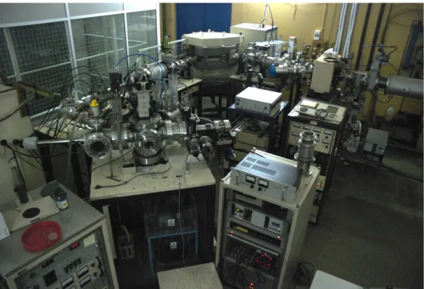
Figure 3.1: 3 MV tandem accelerator at LATR/CTN-ITN.

3.1.1 The target chamber

Figure 3.2 shows a photograph of the target chamber where its main parts are visible. The numbers seen in the photograph identify each main component:

(1) modified HICONEX ion source

(47)

3.1.1.1 Ion source

The general Ionex Model 834 HICONEX cesium ion source was modified to allow for the production of a positively charged cesium microbeam.

Figure 3.2: Micro-AMS chamber at LATR/CTN-ITN. In this image it is visible the ion source on the left side behind the vacuum lock system, the microscope on top of the chamber. The smaller circular glass window on the main chamber allows the operator to view the target holder.

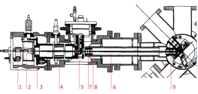
In figure 3.3b a drawing of the ion source main components is shown, with numbers associated to each component.

(48)

the ionizer tube (2) that can be heated up to 1100 ºC, where it will ionize. The positively ionized cesium will be injected into the extraction zone (3) that is polarized at around -5600 V. After this area there are four semi-cylindrical plates (each a 1/4 of a cylinder) that can be polarized up to 1000 V. These are called the focus lens (4). They can adjust the trajectory of the positively ionized cesium beam. In a normal Hiconex 834 source the cesium beam would, after the focus lens, hit the target, which would be mounted on a 12-position revolver (5) and polarized at -5 kV.

Figure 3.3: b) Scheme of the interior of the modified hiconex ion source.

(49)

used. At this beam size, the primary beam intensity is about 16 nA, and 120 nA at 100 µm beam diameter, corresponding to a 1.6 mA/cm2_[1]

.

3.1.1.2 Main chamber

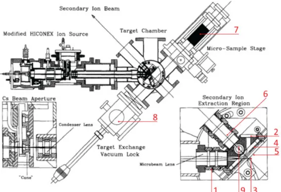
In figure 3.4 a general scheme of the center of the target chamber is shown, where the target is located. The number is brackets in the following text refer to the numbers shown in this figure.

(50)

Figure 3.4: General scheme of the target chamber.

The target holder is supported in place by a rod that is connected to a Vacuum Generator OMNIAX 3 axis microstage (7), that allows for the sample holder to move in all three spatial dimensions in steps as small as half a micrometer. This of course is a very important feature because it allows the user to analyze the sample in the x and y directions and to analyze different spots of the target even if they are very near each other. Also connected to the target chamber is the vacuum lock system (8) that allows for the quick exchange of targets without a severe loss of the vacuum quality. With this system it is possible to recuperate the initial vacuum conditions after only about fifteen minutes of a target exchange. The target chamber is usually at a pressure of 3 x10-7_mbar. When the ion source is operating the pressure in the target chamber rises to about 1 x 10-6_mbar.

(51)

target into an Olympus SZHIO zoom microscope with a 71 mm working distance situated outside and above the chamber, as can be seen in figure 3.2. Since the prism or mirror is located in front of the target, it was designed with a cylindrical aperture in its center so that the secondary beam can pass through it. The microscope is connected to a camera that captures the image of the target in real time and sends it to the control computer. With a x10 ocular, a total maximum magnification of 70 is obtained. This is further magnified using a web camera, approximately by a factor of 2, resulting in_{a 1}µm pixel resolution

on the computer screen.

The computer also controls all the different electrostatic focusing and deflecting devices in the chamber and along the beam line, besides the low and high-energy magnets. It also controls the bouncing system that will be described later, and the several faraday cups along the line as well as the detectors in the detector chamber. The control program was developed in Labview software. The control hardware consists of an OMRON PLC system and a few other devices that will also be described later.

3.1.2 The beam transport system

(52)

The LE and HE beam transport systems will be described, following the path of the beam from the target chamber to the detector chamber in the end of the system.

3.1.2.1 The Low-energy (LE) beam transport system or injection system

The LE beam transport system is shown in figure 3.5. In figure 3.6 a general scheme, showing all the main components of this part of the micro AMS system is shown. The numbers in brackets in the following text refer to the numbers shown in this figure.

Figure 3.5: General view of the injection system at LATR/CTN-ITN.

(53)

energy before the accelerator is 10 keV, which is a low energy compared with the beam's energy after the accelerator.

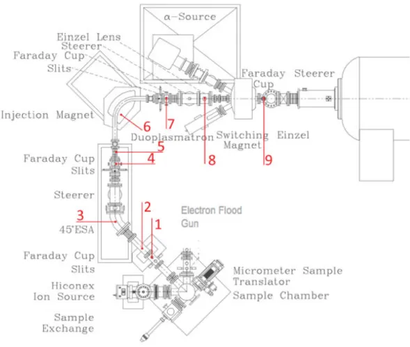
As was described before, the secondary einzel lens focuses the secondary beam exiting the extractor block in the target chamber. This lens was specially dimensioned so that its image is located in the same point as the object of the LE ESA (low energy electrostatic analyzer). At this point there is the first set of slits and faraday cup (FC) (1). Using these slits and FC it is possible to optimize all the devices in the target chamber, before feeding the beam through the LE ESA. After this first set of slits there is another set (2) that reduces beam halo. When all the electrostatic devices in the target chamber are optimized, the first FC is lowered and the beam proceeds to the LE ESA (3).

(54)

Figure 3.6: General scheme of the injection system, with all its different elements.

(55)

After this chamber the selected mass will proceed through the so-called image einzel (8). This einzel lens focuses the beam in the last FC (9) before the beam enters the accelerator. When this LE FC is lowered the beam enters the accelerator and is measured in the FC after the accelerator (HE FC). Between these two faraday cups there are a few electrostatic elements that have to be optimized, both at the entrance and at the exit of the accelerator. On the low energy side, there are two sets of lenses; the matching lenses and the tube lenses and a set of x and y deflector plates. On the high-energy side there are a set of x and y deflector plates and a set of X and Y focusing electrostatic quadropoles.

The stripping system is controlled at the accelerator’s main console and consists of a step-by-step motor that controls the valve of an argon gas bottle located inside the accelerator tank. This valve is connected to a tube that feeds the argon gas to the accelerator tube.

(56)

Danfysik magnet (visible below the second light counting from the left on the top of the image). Also visible in this image are two other beam lines that do not belong to the high-energy beam transport line branching from the second switching magnet that appears just below the accelerator in the image. The first switching magnet is the first magnet after the accelerator.

3.1.2.2 The High-energy (HE) beam transport system

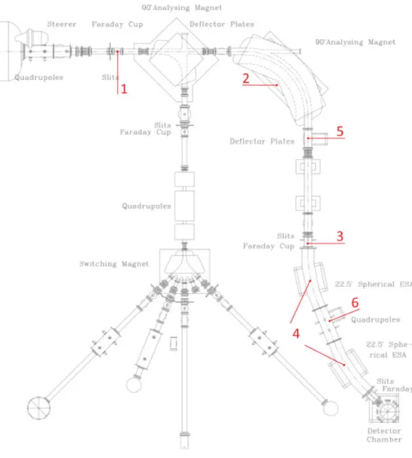
The HE beam transport system can be seen in figure 3.7. In figure 3.8 a general scheme shows all the main components of this part of the micro AMS system. The numbers in brackets in the following text refer to the numbers shown in this figure.

As mentioned previously, there will be a predominantly mono-atomic beam after the accelerator, with several positive charge states. After the HE FC (1) is lowered, the beam proceeds to the 1.3 m radius HE magnet (2), which was built by Danfysik, and is corrected to the second order with a nominal maximum beam product (mE/q2_{) of 140 MeV/amu, although it can work up to}

10% above the specifications, which allows for analysis of mass 240 at 15 MeV (5+ charge state at 2.5 MV terminal voltage) [3]. The pole tips have a 3 cm gap and are 15 cm wide and have between them a 10 cm wide by 2.5 cm high stainless steel beam box, which allows at least ± 10 amu latitude in transmission at mass 240. The magnet power supply is provided by a Danfysik model 858 current supply regulated to 1 ppm.

(57)

After the Danfysik cups the beam passes thru a pair of 3 m radius ESAs (4), each with a 22,5º bend, that will work as energy filters as in the LE side. In order to correct possible misalignments of the beam between the exit channel of the magnet and the detector chamber, a set of X and Y electrostatic quadrupoles (5) is located after the magnet and again between the two ESAs (6). The quadupole between the ESAs has the double purpose of maintaining the beam envelope bellow 25 mm and keeping the ESA voltages below 50 kV thus avoiding hazardous X-ray background.

3.1.2.3 The Electrostatic Analyzers (ESA´s)

The LE ESA is a 45º curved tube, which encloses two curved plates (they are curved both horizontally and vertically) which are polarized with opposite fixed voltages (usually around 1000 V). The spherical shape of the plates will focus the beam both horizontally and vertically, making the ESA a double focusing device.

In the high energy side of the system two more ESA´s are used. All ESA’s are used for the same goal and work using the same principle, that will be briefly explained.

An electrostatic field is created between the two plates, separated by distance

d, via the application of opposite polarity voltages on each of its plates, thus creating a potential difference ΔV. An ion passing through this electrostatic field will have a centripetal force acting upon it:

F=q q =2E/r

(58)

For a cylindrical analyzer, ions with the same E/q value will follow concentric paths inside the ESA, while unwanted ions with different E/q values will undergo trajectories with a different r, exiting the ESA with a deflection Δy from the central radius r :

Δ!∼!

ℇ_!!

4!

where L is the length of the plates.

Since it is important to maximize Δy, the size of the ESA, L, should be as large as possible, depending on the beam energy and charge state selected. The ESA will permit a control of the energy distribution. A 45º bend spherical electrostatic analyzer operating in the double focusing mode has a dispersion of

(59)

Figure 3.8: General scheme of the High-energy beam transport system with all its different elements.

3.1.2.4 The stripper

(60)

mono-negative ion are removed when the ion interacts with a gas at a certain pressure inside a tube in the center of the accelerator (called stripper channel), thereby changing the ion's polarity. This change in polarity allows for achieving particle final energies !! =!! + !+1 .!.!! , as a particle will be accelerated

towards the center of the accelerator while entering the accelerator tube at charge state -1 and then again pushed towards the exit channel of the accelerator, by the same terminal voltage +V, after changing its polarity to +n in the stripping channel. This means that a tandem of 3 MV terminal voltage (TV) as the one in LATR will be able to accelerate heavy ions to several MeV of energy (ex: 110_Ag7+_{ions will achieve a final energy of 24 MeV at}_TV_{= 3 MV).}

Another feature that is of crucial importance to AMS is that molecules become unstable in the stripper channel and molecules in charge states above 2+ will dissociate into their atomic counterparts. This resolves the molecular interferences that plague other mass spectrometry techniques like SIMS and is one of the main advantages of the AMS technique. The other is that the very high energies attainable with relatively low terminal voltages allow for isobar separation using ionization chambers as will be explained further down the text.

The ion charge state after exiting the stripper channel depends on a number of factors that affect the stripper efficiency, such as the gas itself, it's pressure and the terminal voltage of the accelerator. Besides gas stripping, sometimes a solid stripper is used, usually a thin foil of carbon or other material. This usually allows for reaching higher final charge states for the same terminal voltage when compared with gas stripping but also increases beam energy straggling.