The thickness of the transport layer in stratified geomorphic flows

1 INTRODUCTION

Flows with high geomorphic potential, herein geomorphic flows, develop frequently a layered structure with intense sediment transport in the lowermost flow region. A large number of flows can be included in this category, including river flows in the upper regime exhibiting sheet flow and flows resulting from dam or dyke breaking or breaching. These flows have in common the ultimate driving mechanism, gravity, ii) and the fact that they are slender flows and the importance of the micromechanical characteristics of the sediment in the definition of the constitutive equations. The dynamics of the transport layer is thus determined by grain-scale interactions between the granular and the fluid phase. In general, these interactions can be classified as collisional, frictional and viscous (e.g. Iverson 1997).

The theoretical body for granular flows is well established within the dense limit of the

Chapman-Enskog kinetic theory (Chapman & Cowling 1970). However, simple relations for the collisional stress tensor are not possible without a good number of approximations and hypothesis (Savage & Hutter 1989, Jenkins & Richman 1985, Jenkins & Hanes 1998). When the solid concentration exceeds a certain value, interparticle friction plays an important role. Kinetic theories have been modified to account for these effects (Nott & Jackson 1992, Jenkins 2006). The presence of an interstitial viscous fluid has not yet been incorporated with sufficient degree of completeness in spite of theoretical advances (Jenkins & Hanes 1998) and experimental work (Armanini et al. 2005). Some solutions have been proposed including viscous effects. Berzi & Jenkins (2008a,b) have used a linearized version of the phenomenological rheology proposed by GDR MiDi (2004) to obtain analytical solutions to the steady, fully developed flow of a granular-fluid mixture over an erodible bed. Explicit translation of collisional-dominated rheologies of mixtures of granular material and viscous fluids into closure models for shallow-flow

advection-The thickness of the transport layer in stratified geomorphic flows

Rui M.L. Ferreira

CEHIDRO–Instituto Superior Técnico, TULisbon, Portugal, ruif@civil.ist.utl.pt

João G.A.B. Leal

FCT–New University of Lisbon & CEHIDRO–Instituto Superior Técnico, Portugal, jleal@fct.unl.pt

António H. Cardoso

CEHIDRO-Instituto Superior Técnico, TULisbon, Portugal, ahc@civil.ist.utl.pt

ABSTRACT: This paper is aimed at the development of a model for the thickness of the transport layer in stratified geomorphic flows such as sheet-flows or immature debris flows occurring, for instance, as a consequence of dam failure. These are flows with high geomorphic potential, occurring at or generating high shear stresses, whose ultimate driving mechanism is gravity. The micromechanical characteristics of the sediment and viscous flow-grain interactions are of paramount importance in the definition of the constitutive equations that relate stresses and shear rates within the flow. The model was derived from the granular flow theory based on Chapman-Enskog’s dense gas kinetic theory. A 2DV conceptual model was employed to render the flow structure in a flow in the absence of longitudinal pressure gradients. The 2DV model was further simplified to obtain an implicit formula for the thickness of the transport layer. The role of the flux of fluctuating particle energy and of the granular temperature is clarified. Results of the simplified formula are discussed and compared with the result of the complete model. Solutions of hyperbolic instantaneous dam-break problems over mobile beds, incorporating the present model of the transport layer thickness, are presented.

Keywords: Granular-fluid flows, Sheet flows, Granular temperature, Contact load

dominated stratified flows have been attempted by Ferreira (2008) and Ferreira et al. (2009).

The objective of this paper is to present the detailed development of a model for the thickness of the transport layer in stratified geomorphic flows such as sheet-flows or immature debris flows. The model is based on the granular flow theory rooted on Chapman-Enskog’s dense gas kinetic theory, namely from the equation of conservation of fluctuating kinetic energy, incorporating viscous and frictional effects.

Section 2 is dedicated to the description of the physical system and to the presentation of the steady state solution of the conservation and constitutive equations of the granular-fluid flow over an inclined bed. Section 3 presents the main steps that conduct to the formula of the steady-state thickness of the transport layer, from the simplified solution of depth-averaged equation of conservation of the fluctuating kinetic energy. Section 4 presents a discussion of the simplified model. The paper is closed by a Conclusion and recommendations.

2 THE PHYSICAL SYSTEM

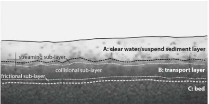
Sheet-flow is a two-dimensional stratified flow involving a mixture of water and granular material, picked up from the bottom. The granular phase is composed of cohesionless sediment grains, nearly elastic, slightly rough and approximately spherical. The fluid is viscous and incompressible. The flow structure is depicted in Figure 1. Three main layers are identified: A, characterized by small mean sediment concentrations or by clear water and where turbulent stresses are dominant; B, a transport layer featuring decreasing concentrations upwards and stresses mainly originated in the granular phase; and C, the bed composed of grains with no appreciable horizontal mean motion.

Figure 1. Detail of a sheet-flow with highlighted idealized layered structure.

In layer B, it is expected that granular collisional stresses are dominant except in a thin bottom boundary layer where frictional stresses

are dominant. Within the framework of the Chapman-Enskog theory, it is possible to derive the equations of conservation of mass, momentum and energy (associated to the fluctuating motion) for the granular phase (details in Ferreira 2005, pp. 231-250) in layer B. In steady flows, these can be written, respectively, as

( ) ( )

, 0

g g

i i

u

ρ ν = (1)

( ) ( ) ( )

, 0

g g gw

ij i j j

T + ρ νg + f = (2)

( ) ( ) ( )

, , 0

g g gw

i i Tij uj i

−Φ + − γ = (3)

where

(

)

( ) ( ) ( ) ( )

, ,

g g g g

ij i j j i

T = μ u +u (4)

is the granular stress tensor, ρ( )g

is the particle density,

ν is the solid fraction (concentration at a specific

point in the flow), ( )g

i

u stands for the granular velocity

field, g is the acceleration of gravity,

( )

(

)

1

( ) 1/2 ( ) ₂

1 3 8 / 5

g g

s

d

μ = π ρ νϑ ϑ Θ is the granular

viscosity, Θ =1₃ c c'_i '_i is the granular temperature,

'_i

c is the fluctuating component of the particle

velocity,

( )

,

g

i K j

Φ = Θ (5)

is the flux of fluctuating energy,

(

)

1

( ) 1/2 ( ) ₂

1 4 4 /

g g

s

K = π ρ νϑ ϑ d Θ is the granular thermal conductivity (or granular diffusivity),

(

)

3

(

)

( ) ( ) ( ) ₂ 1/2

1

24 1 /

gw g gw

s

e d

γ = ρ − νϑ Θ π (6)

is the rate of dissipation (due to inelastic collisions and viscous damping) of the fluctuating energy,

(gw) j

f is the force per unit volume encompassing the interaction (essentially of viscous nature) of the fluid and granular phases and buoyancy, ds is

characteristic diameter of the grains, ϑ₁, ϑ₂, ϑ₃ and ϑ₄ are functions of the solid fraction (details in Ferreira 2005, p. 246) and (gw)

e is the immersed restitution coefficient (Ferreira 2005, p. 248).

It should be noted that the granular normal stresses are isotropic, hence reduced to the granular pressure, ( ) ₁ ( )

3

g g

ii

P = − T , calculated by the equation of state

(

)

( ) ( )

1

1 4

g g

P = νρ + ϑ Θ (7)

approximation (see details in Jenkins & Richman 1988, Ferreira 2005, pp. 231-238).

The equation of conservation of fluctuating energy, Eq. (3), reveals that, unlike thermodynamic systems where every given constant temperature can be made to correspond to an equilibrium state, a granular system can maintain a steady state of agitation, characterized by a given granular temperature, if and only if the rate of production ( ( ) ( )

,

g g

ij j i

T u ) equals the diffusive flux and the dissipation, i.e. if ( ) ( ) ( )

, ,

g g gw

i i ij j i

T u = Φ + γ .

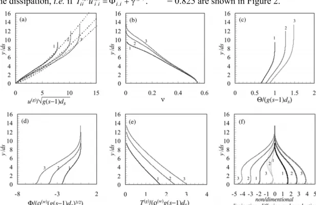
A detailed characterization of the two-dimensional (vertical) flow in layer B is obtained by solving numerically a set of ODEs including equations (2) to (7) and the equations of conservation of momentum of the fluid phase, subjected to appropriate boundary conditions (details in Ferreira 2008). Solutions reproducing experimental conditions of Sumer et al. (1996), namely plastic pellets with ds = 0.003 m, specific

density s = 1.27 and dry coefficient of restitution e = 0.825 are shown in Figure 2.

Figure 2. Computed profiles of the relevant non-dimensional quantities in the transport layer. (a) Velocity of the granular constituent. (b) solid fraction. (c) granular temperature. (d) flux of fluctuating energy. (e) granular shear stresses. (f) dissipation (negative, normal thickness), diffusion (thin lines) and production (positive, thick lines) of fluctuating energy; production is considered positive while diffusion and dissipation are negative. Simulations 1, 2 and 3 correspond to, respectively, θ = 1.74, θ ≈ 2.49 and θ ≈ 3.07.

It was found that the immersed restitution coefficient is ( )

0.005

gw

e = −e θ where

(

( )

)

( ) w ( 1)

b s

T Y g s d

θ = ρ − is the Shields parameter, where y is the vertical coordinate and Y_b is the bed elevation. It is observed that the solid fraction increases almost linearly with the flow depth (Fig. 2b). The shear stress is not constant in the transport layer (Fig. 2e) because its work must balance that of the force of gravity in the direction of the flow. The modulus of the flux of the fluctuating kinetic energy increases towards the bed (Fig. 2d). This means that fluctuating energy is constantly being extracted from the mean flow and directed towards the bottom. As a consequence, the frictional sub-layer cannot increase indefinitely with increasing values of the Shields parameter and consequent increasing normal stresses.

The flux of fluctuating energy is, as required, zero at a large distance form the bed, as the system

3 CLOSURE EQUATIONS FOR THE TRANSPORT LAYER

The integration of the equation of conservation of the fluctuating energy, equation (3), over the contact load layer reads

( ) ( )

d d d d d 0

s s g g s

b b b

Y Y Y

y yx y x

Y Y T u Y

−

∫

Φ ξ +

∫

ξ −

∫

γ ξ = (8)

where Φ is the flux of fluctuating energy, Ys is

the elevation of the top of the transport layer Considering that the flux of fluctuating energy is zero at the boundary between the suspended sediment and the contact load layers and applying the Leibnitz rule, it is obtained

( ) ( ) ( ) ( )

d d 0

s s

g g g g

b b b

Y Y

yx x c c x y yx

Y ⎡T u ⎤Y h Y u T

Φ +_{⎣ ⎦} − γ −

∫

ξ = (9)

where γc is the depth-averaged rate of

dissipation and hc is the thickness of the transport

layer. Assuming that the shear stress associated to the granular phase is approximately linear (Fig.

2e)

( )

( )

(

)

d g d 1

y Tyx = τbc y −y h = − τbc h, being h

the flow depth, and that the velocity at the bed is

( )

0

g

b x _{y Y}

u ₌ = , Eq. (9) becomes

1 0

b

top top

c c c

b c c c

Y

c c

u h u

u h

u h u

⎡ ⎛ ⎞⎤

Φ + τ _⎢ − _⎜ − _⎟⎥− γ =

⎝ ⎠

⎣ ⎦ (10)

where ( )

s

g top c x

Y u =u .

The vertical velocity distribution in the contact load layer can be approximated by the empirical estimate of Sumer et al. (1996). Hence, the depth-averaged velocity is

(

)

3 1 ₄ 4 10 1 7 c c s s h u g s d

d

− ⎛ ⎞

= − _{θ ⎜ ⎟}

⎝ ⎠ (11)

and

(

)

3 1 ₄ 4 5 1 2 top c c s s h u g s d

d

− ⎛ ⎞

= − _{θ ⎜ ⎟}

⎝ ⎠ (12)

so that utopc uc=7 4. Introducing (11) and (12), Eq.

(10) becomes

( )

₍

₎

3

3 4

2

10 7 3

1

7 4 4

0

b

w c c

s Y

s

c c

h h

g s d

d h

h

⎛ θ ⎛⎞ ⎞

Φ + ρ ⎡_⎣ − _{⎤ ⎜⎦ ⎟ ⎜} − _⎟−

⎝ ⎠

⎝ ⎠ − γ =

(13)

The averaged value of the rate of dissipation is

( )

(

)

( ) ₃

2 1 1 ₀ 2 1 d

24 1 ₁

d s b c Y c _Y c gw g h c s y h e h d

γ = γ

− ρ

= νϑ Θ ξ

π

∫

∫

(14) where

( )

3 1 2 2 2 1 0 1 d O c h

c c c

c

C G C

h

∫

νϑ Θ ξ = Θ + (15)

and where G=C_c

(

2−C_c

) (

(

2 1−C_c

)

3

)

is the counterpart of Carnaham & Starling_’s (1969) radial distribution function for averaged quantities, Cc is the mean sediment volumetric

concentration in the contact load layer.

The shear efficiency number, ℜ (Savage & Jeffrey 1981), is a measure of the correlation between the generation of collisional stresses and the state of agitation of a granular system, measured by the fluctuation velocity field. It can be interpreted as a measure of the efficiency of the shear work in generating a particular state of agitation. This number will take on different values depending on the properties of particles, namely their coefficients of restitution and of skin friction. ℜ is Ord(1) for intermediate solid fractions, is much smaller than 1 for dilute systems and is much larger than 1 for dense systems. Parameter ℜ can be re-written as

( )

1 1 1

2 2 2

d ₇

4

top

y x c c c c

s s s

c c

u u h u h

d d d

ℜ = ≈ =

Θ Θ Θ

(16)

and can be used to relate the granular temperature and the depth-averaged velocity, as

3 3 2 7 4 c c c s u h d ⎛ ⎞

Θ = ⎜_{⎝ ℜ} ⎟_⎠ (17)

The mean sediment volumetric concentration can be obtained, under capacity conditions, from the integration of the equation of conservation of fluctuating kinetic energy in the frictional layer (details in Ferreira 2005, pp. 279-280), rendering

( )

tan s c b c d C h θ =

ϕ (18)

(

)

( )

( )

(

)

2 1 3 2 3 1 3 4 4 2

24 5 1

1 2 tan 1 w c c b c s s G

h e s

h g s d

d

− ⎛ ⎞

γ = _{⎜ ⎟} − ρ ×

ϕ ℜ ⎝ ⎠

π

⎛ ⎞

×⎡_⎣ − ⎤_⎦ θ _{⎜ ⎟}

⎝ ⎠

(19)

The flux at the bed is calculated by the formulation of Jenkins & Askari (1991), modified by Ferreira (2005), p. 255

( )

(

)

( )

1 2

4

1/ 2 0

2 30

2 5

3 1 tan

4

gw

b

Q N e

Y b

⎡ _π ⎤

= − Θ ⎢ − − ϕ ⎥ϑ

π _⎢⎣ ϑ _⎥⎦ (20)

where N represents the weight of granular material per unit bed area, i.e. the granular pressure at the bed. Introducing the equation of state for the normal stress at the bed, Eq. (7), and Eq. (18), Eq. (20) becomes ( )

(

)

( )

( )

(

)

( )

3 2 2 0 0 3 0 0 1 tan 5

3 1 tan

4 b w s Y b gw b

g s d

Q

e M

K sG

⎡ − θ⎤

= −ρ _{⎢ ⎥} ×

ϕ

⎢ ⎥

⎣ ⎦

⎡ _{− −} π _ϕ ⎤

⎢ ⎥

⎣ ⎦

×

π ν

(21)

where K0 and M0 are the counterparts of ϑ3 and ϑ4 for averaged concentrations. Introducing (19) and (21) in (13) one obtains

( )

(

)

( )

( )

( )

(

)

( )

_{( )}

2 0 0 3 3 0 0 3 3

3 _{4 2}

4 1 2 1 3 2 5

3 1 tan

4 0.49 tan 7 3 4 4 262.5 1 1 0 tan gw b b

c c c

s s gw c b e M K sG

h h h

d d h

G C

e s −

⎡ _{− −} π _ϕ ⎤

⎢ ⎥

⎣ ⎦

− ×

π ν ϕ

⎛ ⎞ ⎛ _{⎞ ⎛} ⎞

×θ _{⎜ ⎟} +_{⎜ ⎟ ⎜} − _⎟−

⎝ ⎠

⎝ ⎠ ⎝ ⎠

− − θ =

ϕ ℜ π

(22)

Eq. (22) is the closure equation for hc. Notice

that (22) can be written as

( ) (

3₂

)

34

( )

3₄ 12

2 3

; 0

c c c

x χ h h − β θ x − β θ =− where xc =

hc/ds and

(

)

7 3 ; 4 4 c c h h h h

χ = − . The large ℜ limit

corresponds to dense flows with high dissipation of fluctuating energy due, for instance, to viscous effects from an interstitial fluid (Savage & Jeffrey 1981). In this limit, (22) reduces to

4 3 2 c s h d

⎛β ⎞

=_{⎜ ⎟} θ

χ

⎝ ⎠ (23)

which is a linear relation such as the one proposed by Wilson (1987). For typical values of the parameters involved, the slope in (23) varies between 2 and 5.5, which is two to five times smaller than the value proposed by Wilson in his equation h d_{c s} = θ10 . It is thus proposed that the large ℜ limit does not represent the variation of hc

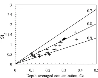
correctly and full equation (22) should be used. The introduction of ℜ in (22) envisaged the introduction of the effects of the granular temperature. Thus, the parameter ℜ, computed with depth-averaged quantities, should be provided independently. Data from Ahn et al. (1992) and from the numerical simulations carried out to produce Fig. 2 are appropriate to estimate the shear efficiency number. Such data is re-plotted in Fig. 3 along with estimates of ℜ, in the form of a family of lines parameterized in terms of (1 − e). Thus, as seen in that figure, the linear relation in the form

(

)

0.65 8 1

1

c

C e

p

ℜ =⎡_⎣ + − ⎤_{⎦ −} (24)

where p is the bed porosity, describes the data fairly well. 0 0.5 1 1.5 2 2.5 3

0 0.1 0.2 0.3 0.4 0.5

Depth-averaged concentration, Cc

R

0.9 0.8 0.7

Figure 3. Solid lines correspond to Eq. (24) with the parameter e taking on the values 0.7, 0.8 and 0.9. Crosses (+) correspond to the dry granular flow data of Ahn et al. (1992). Numerical results for Sumer’s (1996) sediment of type a (◊), and sediment of type b (♦).

4 DISCUSION OF THE THICKNESS OF THE TRANSPORT LAYER

inspection and extrapolation from the solid fraction profile.

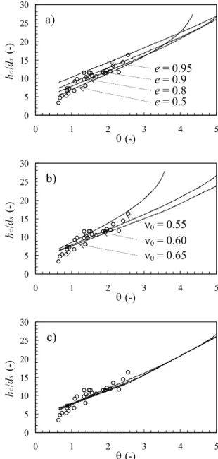
Figures 4 and 5 display the experimental results Sumer etal. (1996) corresponding to visual inspection. It is believed that the extrapolation from the solid fraction, although more susceptible to be compared among researchers, greatly overestimated the thickness of the transport layer. A sensitivity analysis to the values of the restitution coefficient, to the total discharge, q, and to the solid fraction at the bed are performed in Figs. 4a, 4b and 4c. Fig. 4d shows a different kind of sensitivity analysis: several parameters are varied, corresponding to the geometrical and mechanical characteristics of the sediment employed by Sumer etal. (1996).

In agreement with the findings of Zhang & Campbell (1992), the increase of the values of the coefficient of restitution results in an increase in the thickness of the contact load layer. The main effect of decreasing the total discharge while maintaining the bed shear stress is the narrowing of the ratio h d_{c s} , as seen in Fig. 4b. It was also found that the smaller the solid fraction at the bed the larger the values of hc.

The most interesting result expressed in Fig. 4 is the invariance of h d_{c s} as a response to the variation of the type of sediment. If the proper values for the relevant parameters are chosen, namely the restitution coefficient and the internal friction angle at the bed, the non-dimensional thickness of the contact load layer is virtually independent from the type of sediment. In Fig. 5, the specific conditions of the experimental tests of Sumer etal. (1996), namely the discharge rate and the flow depth, are reproduced in the computation of h d_{c s}. The numerical values are efficiently represented by the power law

1.7 5.5

c

s

h

d = + θ (25)

Thus, for faster, yet possibly less accurate, computations, Eq. (22) may be replaced by (25). It is noteworthy that Wilson_’s (1987) equation for the thickness of the sheet-flow, h d_{c s} = θ10 was obtained from an equation such as (18) with Cc =

0.625, the maximum packing of identical spheres, and Bagnold_’s (1954) value of tan(ϕb) = 0.32. Eqs.

(18), (22) and (25) state that the variation of hc/ds

is not exactly linear with the Shields parameter and that the depth-averaged sediment concentration is not exactly constant, as in classic sheet-flow studies (e.g., Wilson 1987, 1989). These results seem to be in a better agreement with the two-dimensional numerical simulations performed previously in section 2.

0 5 10 15 20 25 30

0 1 2 3 4 5

θ (-)

h

c

/

d

s

(-)

0 5 10 15 20 25 30

0 1 2 3 4 5

θ (-)

h

c

/

d

s

(-)

0 5 10 15 20 25 30

0 1 2 3 4 5

θ (-)

h

c

/

d

s

(-)

Figure 4. Thickness of the sheet-flow layer as a function of the Shields parameter. Sensitivity analysis to (a) the restitution coefficient; e = 0.5, 0.8, 0.9 and 0.95; tan(ϕb) = 0.35; ν0 = 0.65; q = 1.0 m2/s; (b) maximum solid fraction at the bed; ν0 = 0.55, 0.60 and 0.65; e = 0.8; tan(ϕb) = 0.4; q = 1.0 m2/s and (c) the characteristics of the sediment grains. The four types of granular material used by Sumer et al. (1996), were plastic (ds = 0.003 m, s = 1.27, e = 0.75 and ds = 0.0026 m, s = 1.14, e = 0.75), acrylic (ds = 0.0006 m, s = 1.13, e = 0.75) and sand (ds = 0.00013 m, s = 2.67, e = 0.8); ν0 = 0.6; tan(ϕb) = 0.4; q = 1.0 m2/s. Circles (○) stand for Sumer’s et al. data.

The results of the full 2DV numerical simulations are also shown in Fig. 5. Comparing with experimental results, it is observed that these simulations underestimate hc for high Shields

numbers. This may be an effect of the techniques used to estimate experimentally the thickness hc.

The agreement between the simplified models Eq. (22) and (25) and the full 2DV model is qualitatively good. The introduction of the simplifications led to an overestimation of hc

relatively to the complete model. (

( a)

b)

c)

e = 0.5 e = 0.8 e = 0.9 e = 0.95

Figure 5. Non-dimentional thickness of the sheet-flow layer. Crosses (+) stand for the results of (22); triangles (Δ) and circles (○) stand for the experimental results of Sumer et al. (1996). Dashed line (- - - -) stands for the results of equation (25). Large circles stand for the results of the full 2DV model. Black circles ( ) stand for plastic (ds = 0.003 m, s = 1.27, e = 0.75) and white circles ( ) stand for acrylic (ds = 0.0006 m, s = 1.13, e = 0.75).

It is noteworthy that Fraccarollo & Capart (2002) used a relation similar to (18) in order to compute the thickness of their transport layer. In order to derive (18), they assume that there is a discontinuous state of shear stress across the interface between the bed and the transport layer. This interface acts like a phase interface and requires that there is a basal slip velocity. At the sharp interface they apply Rankine-Hugoniot shock conditions thus obtaining (18). Fraccarollo & Capart (2002) then assume that the concentration in the transport layer is constant and use (18) to compute hc. The advantage of the

present formulation is that the thickness of the transport layer is computed from an independent formula, using energy considerations, allowing for a variable mean sediment concentration.

5 APPLICATION TO DAM FAILURE TESTS The dam failure experimental results of Ferreira et al. (2006) are used to test the validity of the closure equation for the thickness of the transport layer devised in this paper (Eq. 25). The experiments were composed of different water levels upstream and downstream. The bed was composed of PVC pellets with equal or different levels upstream and downstream. The main features of the experimental tests are presented in Table 1, where hL and hR are the initial water

depth, respectively, upstream and downstream, YbL

and YL are the initial upstream bed and water

levels, respectively. More details can be found in Ferreira et al. (2006).

Table 1. Main features of experiments of Ferreira et al. (2006)

______________________________________________ TEST hL (m) YbL (m) hR (m) YL (m)

______________________________________________

35_00_00 0.35 0.00 0.00 0.35

35_10_00 0.25 _{_____________________________________________} 0.10 0.00 0.35

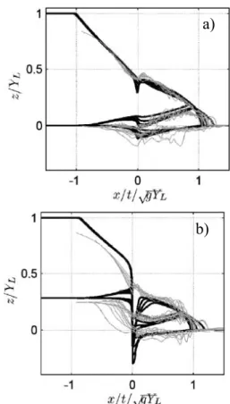
The non-dimensional flow experimental and numerical profiles are presented in Fig. 6. In that figure, x is the longitudinal coordinate, starting in the gate (dam) location, and z is the elevation measured from the initial bed level downstream.

Figure 6. Non-dimensional flow profiles: a) test 35_00_00; b) test 35_10_00. Black lines represent the numerical solutions obtained using Eq. (25) and grey lines stand for experimental dam failure results of Ferreira et al. (2006).

The results presented in Fig. 6 show a reasonable agreement between the calculated (Eq. 25) and the measured thickness of the transport layer. In the region behind the wave-front, where high shear stresses occur, the agreement is better than in low velocity regions, which may indicate that inertial effects, absent in the present formulation, will have to be introduced for a better overall agreement.

6 CONCLUSIONS

The main results of the present work may be summarized as follows.

The thickness of the transport layer may be derived from the equation of conservation of the particle fluctuating energy.

0 2 4 6 8 10 12 14 16 18 20

0.5 1.0 1.5 2.0 2.5 3.0

θ (-)

h

c

/

d

s

(-)

a)

The driving mechanism is similar to that controlling the flow depth in turbulent, uniform (in the longitudinal direction) open-channel flows: the stronger the energy production (in this case due to large coefficient of restitution or otherwise increased granular stresses), the more important the vertical flux of fluctuating energy and the thicker the transport layer to allow for complete energy dissipation.

The proposed model, by introducing the solution of an extra conservation equation, allows for a variable sediment concentration in the transport layer.

Preliminary tests reveal that the normalized thickness of the transport layer may be independent of the bed material.

A simplified model, suitable to be introduced in layered shallow flow models was derived, maintaining the main features of the complete model.

Dam-break simulations, incorporating the proposed model, show a reasonable agreement between the measured and the calculated thickness of the transport layer.

The main differences occur for low velocities, where the model overestimates the thickness of the transport layer. Research is needed in the inertial terms of the equation of conservation of energy to obtain an unsteady flow formula for the thickness of the transport layer.

REFERENCES

Ahn, H., Brennen, C.E. & Sabersky, R.H. 1992. Measurements of velocity, velocity fluctuations, density, and stresses in chute flows of granular materials. J. Appl. Mech., 58, 792-803.

Armanini, A., Capart, H., Fraccarollo, L. & Larcher, M. 2005. Rheological stratification in experimental free-surface flows of granular–liquid mixtures. J. Fluid Mech,, 532, 269-319.

Bagnold, R.A. 1954. Experiments on a gravity-free dispersion of large solid spheres in a Newtonian fluid under shear. Proc. R. Soc. Land. A 255, pp. 49-63. In “The physics of sediment transport by wind and water, a collection of hallmark papers by R. A. Bagnold”. Ed. by Colin R. Thorne, Robert C. MacArthur & Jeffrey B. Bradley. ASCE, 1988.

Berzi, D. & J.T. Jenkins 2008a. A theoretical analysis of free-surface flows of saturated granular–liquid mixtures. J. Fluid Mech., 608, 393-410.

Berzi, D. & J.T. Jenkins 2008b. Approximate analytical solutions in a model for highly concentrated granular-fluid flows. Physical Review E 78, 011304.

Carnaham, N.F. & Starling, K.E. (1969) Equation of state for nonattracting rigid spheres. J. Chem. Phys. 51(2), 635-636.

Chapman, S. & Cowling, T. G. 1970. The Mathematical Theory of Non-Uniform Gases, 3rd Edn. Cambridge University Press.

Ferreira, R.M.L. 2005. River Morphodynamics and sediment transport. Conceptual model and solutions. PhD Thesis, Instituto Superior Técnico, TU Lisbon. Ferreira, R.M.L., Amaral, S., Leal, J.G.A.B. & Spinewine,

B. 2006. Discontinuities in geomorphic dam-break flows. River Flow 2006, Lisbon, Vol. 1; 1521-1530. Ferreira, R.M.L. 2008. Fundamentals of mathematical

modelling of morphodynamic processes. Applicationto geomorphic flows. In Numerical Modelling of Hydrodynamics for Water Resources, García Navarro & Playán Eds. - Taylor & Francis, 189-209.

Ferreira, R.M.L., Franca, M.J., Leal, J.G.A.B. & Cardoso, A.H. 2009. Closure models for the simulation of unsteady open-channel flows with mobile beds based on grain-scale mechanics. Can. J. Civ. Eng., 36, 1605-1621. Fraccarollo, L. & Capart, H. 2002. Riemann wave

description of erosional dam-break flows. J. Fluid Mech. 461, 183-228.

GDR MiDi 2004. On dense granular flows. Eur. Phys. J. E, 14, 341–365.

Iverson, R. 1997. The physics of debris flows. Reviews of Geophysics, 35(3), 245-296.

Jenkins, J.T. 2006. Dense shearing flows of inelastic disks. Phys. Fluids 18, 103307.

Jenkins, J.T. & Askari, E. (1991) Boundary conditions for rapid flows: phase interfaces J Fluid Mech. 223:497-508. Jenkins, J.T. & Richman, M.W. 1988. Plane simple shear of smooth inelastic circular disks: the anisotropy of the second moment in the dilute and dense limits. J. Fluid Mech. 192, 313-328.

Jenkins, J.T. & Richman, M.W., 1985. Kinetic theory for plane flows of a dense gas of identical, rough, inelastic circular disks. Phys. Fluids 28 (12) 3485-3494.

Jenkins, J. T. & Hanes, D. M. (1998) Collisional sheet flows of sediment driven by a turbulent fluid. J. Fluid Mech. 370: 29-52.

Nott, P. & Jackson, R., (1992) Frictional-collisional equations of motion for granular materials and their application to flow in aerated chutes. J. Fluid Mech. 241, 125-144.

Savage, S. B. & Hutter, K. 1989. The motion of a finite mass of granular material down a rough incline. J. Fluid Mech. 199, 177-215.

Savage, S.B. & Jeffrey, D.J. 1981. The stress tensor in a granular flow at high shear-rates. J. Fluid Mech. 110, 255-272.

Sumer, B.M., Kozakiewicz, A., Fredsøe, J. & Deigaard, R. 1996. Velocity and Concentration Profiles in Sheet-Flow Layer of Movable Bed. J. Hydraul. Eng., 122, 549-558. Wilson, K.C. 1987. Analysis of bed-load motion at high

shear stress. J. Hydraul. Eng., 113(1), 97-103.

Wilson, K.C. 1989. Mobile-bed friction at high shear stress. J. Hydr. Engrg., 115(6), 825–830.