Explaining the predictions of a boosted tree algorithm : application to credit scoring

EXPLAINING THE PREDICTIONS OF A BOOSTED

TREE ALGORITHM

Pierre Antony Jean Marie Salvaire

Application to Credit Scoring

Dissertation presented as partial requirement for obtaining the

Master’ degree in Statistics and Information Management

NOVA Information Management School

Instituto Superior de Estatística e Gestão de Informação

EXPLAINING THE PRDICTIONS OF A

BOOSTED TREE ALGORITHM

A

PPLICATION TO

C

REDIT

S

CORING

by

Pierre Antony Jean Marie Salvaire

Dissertation report presented as partial requirement for obtaining the Master’s degree in

Information Management, with a specialization in Business Intelligence and Knowledge

Management

Supervisor: Rui Goncalves

ABSTRACT

The main goal of this report is to contribute to the adoption of complex « Black Box » machine learning models in the field of credit scoring for retail credit.

Although numerous investigations have been showing the potential benefits of using complex models, we identified the lack of interpretability as one of the main vector preventing from a full and trustworthy adoption of these new modeling techniques. Intrinsically linked with recent data concerns such as individual rights for explanation, fairness (introduced in the GDPR1_{) or model reliability, we believe that this kind of research is crucial for easing its}

adoption among credit risk practitioners.

We build a standard Linear Scorecard model along with a more advanced algorithm called Extreme Gradient Boosting (XGBoost) on a retail credit open source dataset. The modeling scenario is a binary classification task consisting in identifying clients that will experienced 90 days past due delinquency state or worse.

The interpretation of the Scorecard model is performed using the raw output of the algorithm while more complex data perturbation technique, namely Partial Dependence Plots and Shapley Additive Explanations methods are computed for the XGBoost algorithm.

As a result, we observe that the XGBoost algorithm is statistically more performant at distinguishing “bad” from “good” clients. Additionally, we show that the global interpretation of the XGBoost is not as accurate as the Scorecard algorithm. At an individual level however (for each instance of the dataset), we show that the level of interpretability is very similar as they are both able to quantify the contribution of each variable to the predicted risk of a specific application.

KEYWORDS

Credit Scoring, XGBoost, Model Interpretation, Black Box

TABLE OF CONTENT

1 INTRODUCTION AND MOTIVATIONS ... 1

1.1 CREDIT SCORING ... 1

1.2 CHALLENGER MODELS:POTENTIAL BENEFITS ... 2

1.3 “BLACK BOX”DILEMMA ... 4

1.4 PROPERTIES OF INTERPRETATIONS ... 6

1.5 MOTIVATIONS AND METHODOLOGY ... 7

2 DATA DESCRIPTION AND CLEANSING ... 9

2.1 DATA DISCOVERY ... 9

2.2 MISSING VALUES ... 10

2.3 OUTLIERS ... 11

3 VARIABLE SELECTION AND DATA PARTITIONING ... 15

3.1 UNIVARIATE GINI INDEX ... 15

3.2 CORRELATION ANALYSIS ... 15

3.3 SAMPLING:MODEL TRAINING AND TESTING ... 18

4 MODELLING TECHNIQUES ... 20

4.1 SCORECARD ... 20

4.1.1 Logistic Regression ... 20

4.1.2 Scorecard ... 22

4.2 XGBOOST ... 27

4.2.1 CART - Decision Tree ... 27

4.2.2 Ensemble Models ... 29 4.2.3 Gradient Boosting ... 30 5 HYPER-PARAMETERS OPTIMIZATION ... 32 5.1 BAYESIAN OPTIMIZATION ... 32 5.2 PRACTICAL APPLICATION... 33 6 MODELS EVALUATION ... 35

6.1 RECEIVER OPERATING CHARACTERISTIC CURVE ... 35

6.2 LOG-LOSS (LOGARITHMIC LOSS) ... 36

7 XGBOOST INTERPRETATION TECHNIQUES ... 37

7.1 PARTIAL DEPENDENCE PLOTS (PDP) ... 37

7.2 SHAP (SHAPLEY ADDITIVE EXPLANATIONS)VALUES ... 39

8 RESULTS AND DISCUSSION... 41

8.1 STATISTICAL RESULTS ... 41

8.2 GLOBAL INTERPRETATION ... 43

8.3 LOCAL INTERPRETATIONS ... 48

8.4 STABILITY ANALYSIS ... 52

9 CONCLUSION AND FUTURE WORK ... 56

10 BIBLIOGRAPHY ... 58

LIST OF FIGURES

FIGURE 1:AIADOPTERS SEGMENTATION (COLUMBUS,2017) ... 3

FIGURE 2:THE TWO FACES OF AI-BASED CREDIT SCORES ... 3

FIGURE 3:AGE DISTRIBUTION ... 12

FIGURE 4:DEBT RATIO DISTRIBUTION ... 12

FIGURE 5:NUMBER OF DEPENDENTS DISTRIBUTION ... 13

FIGURE 6:NUMBER OF TIMES 90DAYS LATE DISTRIBUTION ... 13

FIGURE 7:MONTHLY INCOME DISTRIBUTION ... 13

FIGURE 8:REVOLVING UTILIZATION OF UNSECURED LINES DISTRIBUTION ... 14

FIGURE 9:CORRELATION BETWEEN 10 VARIABLES (NUMERIC TABLE IN ANNEX Nº2)... 16

FIGURE 10:CORRELATION BETWEEN 7 VARIABLES (NUMERIC TABLE IN ANNEX Nº3)... 17

FIGURE 11:HOLDOUT TRAIN TEST SPLIT ... 18

FIGURE 12:VALIDATION AND TESTING METHODOLOGY ... 19

FIGURE 13:LINEAR REGRESSION ... 20

FIGURE 14:BINARY PROBLEM REPRESENTATION ... 21

FIGURE 15:LOGISTIC REGRESSION ... 21

FIGURE 16:EXAMPLE SCORECARD (ANDERSON,2007) ... 23

FIGURE 17:BINNING OF AGE VARIABLE (ANDERSON,2007) ... 24

FIGURE 18:WOE AND LOGICAL TRENDS (ANDERSON,2007) ... 25

FIGURE 19:DECISION TREE ... 27

FIGURE 20:ENSEMBLE OF DECISION TREE ... 29

FIGURE 21:ILLUSTRATION OF A BAYESIAN OPTIMIZATION PROCESS ... 32

FIGURE 22:RECEIVER OPERATING CHARACTERISTIC CURVE ... 35

FIGURE 23:LOGARITHMIC LOSS ... 36

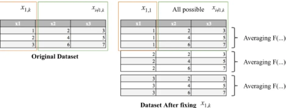
FIGURE 24:PDPCALCULATION -SIMPLIFIED REPRESENTATION ... 37

FIGURE 25:PDPCALIFORNIA HOUSING DATASET EXAMPLE ... 38

FIGURE 26:“ILLUSTRATION OF THE DIFFERENCE IN MODEL PERFORMANCE THAT WE WANT TO FAIRLY DISTRIBUTE AMONG THE FEATURES …”.(CASALICCHIO ET AL,2018)... 39

FIGURE 27:SHAP INDIVIDUAL FEATURE CONTRIBUTION ... 40

FIGURE 28:TEST SETS ROC AUC CURVES ... 41

FIGURE 29:GINIS TRAIN VS TEST SET ... 42

FIGURE 30:LOG-LOSS TRAIN VS TEST SET ... 42

FIGURE 31:SCENARIO SIMULATION ... 43

FIGURE 32:CLASSICAL FEATURE IMPORTANCE –XGBOOST ... 45

FIGURE 33:SHAP FEATURE IMPORTANCE ... 46

FIGURE 34:PARTIAL DEPENDENCE PLOTS ... 47

FIGURE 35:XGBOOST -DISTRIBUTION OF PREDICTED PROBABILITY &SHAP BASE VALUE ... 50

FIGURE 36:HIGH-RISK INDIVIDUAL EXPLANATION ... 50

FIGURE 37:LOW-RISK INDIVIDUAL EXPLANATION ... 51

FIGURE 38:HIGH-RISK PERTURBED INDIVIDUAL INTERPRETATION ... 53

FIGURE 39:LOW-RISK PERTURBED INDIVIDUAL INTERPRETATION ... 54

FIGURE 40:DISTRIBUTION OF CONTRIBUTION VARIATIONS ACROSS ALL VARIABLES ... 55

LIST OF TABLES

TABLE 1DATA DICTIONARY ... 9

TABLE 2 :DEFAULT RATE ANALYSIS ... 10

TABLE 3 :DESCRIPTIVE STATISTICS ... 10

TABLE 4 :MISSING VALUES ... 11

TABLE 5:UNIVARIATE GINI ... 15

TABLE 6:AGE VARIABLE FINAL ENCODING ... 26

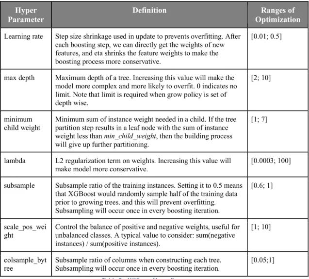
TABLE 7:XGBOOST HYPER PARAMETERS ... 33

TABLE 8:SCORECARD HYPER PARAMETERS ... 34

TABLE 9: STATISTICAL EVALUATION ... 41

TABLE 10:SCORECARD COEFFICIENTS ... 44

TABLE 11:SCORECARD INTERPRETATION OVERVIEW ... 44

TABLE 12:LOW AND HIGH-RISK APPLICATION CHARACTERISTICS ... 48

TABLE 13:SCORES LOW AND HIGH-RISK APPLICATION ... 49

TABLE 14:FINAL SCORECARD TABLE ... 49

TABLE 15:PERTURBED DATA POINTS ... 52

TABLE 16:PERTURBED SCORES ... 52

TABLE 17:SCORECARD BINNING PROCESS RESULTS ... 63

TABLE 18:NUMERIC CORRELATION TABLE -10VARIABLES ... 64

TABLE 19:NUMERIC CORRELATION TABLE -7VARIABLES ... 65

TABLE 20:HIGH-RISK &LOW-RISK INDIVIDUAL EXPLANATION (FIGURE 36&37) ... 66

TABLE 21:HIGH-RISK &LOW-RISK INDIVIDUAL PERTURBED EXPLANATION (FIGURE 38&39) ... 66

LIST OF ABBREVIATIONS AND ACRONYMS

PDP: Partial Dependence Plot

SHAP: SHapley Additive exPlanations XGBoost: eXtreme Gradient Boosting WoE: Weight Of Evidence

Roc Auc: Area Under the Curve

GDPR: General Data Protection Regulation PD: Probability of Default

1 Introduction and Motivations

1.1 Credit Scoring

Credit scoring can be defined as a quantitative method used to measure the probability that a loan applicant or existing borrower will default (Gup & Kolari, 2005). For each individual, a score is calculated according to the probability of default that was given by a statistical model. The final score is most commonly based on demographic characteristics and historical data on payments. During the modeling process, the algorithm identifies and learns how these characteristics are related to credit risk. Later on, the algorithm applies these patterns to a new population and assigns a score to a new customer. Low scores correspond to very high risk, and high scores indicate almost no risk.

After defining a score for each individual, the decision maker has to choose a cutoff score above which loan applications will be rejected. This decision is made according to the risk appetite and strategy that one wishes to put in place. “These techniques decide who will get credit, how much credit they should get and what operational strategies will enhance the profitability of the borrowers to the lenders” (Thomas et al., 2002).

Credit scoring applications in banking sector have expanded during the last 40 years (Banasik and Crook, 2010), especially due to the growing number of credit applications for different financial services, among which consumer loans is considered to be one of the most important and essential in the field (Sustersic et al., 2009).

In this growing environment, the need for an automated credit scoring process over the global financial system have been a key driver of the development of credit scoring techniques. As a result, banks developed industry standards for building, evaluating and regulating models and credit scoring processes. Scorecards models, based on Logistic Regression algorithm, became the most widely used tool for building scoring models (Abdou & Pointon, 2011 - Thomas, Edelman & Crook, 2002, p27 - Siddiqi, 2017).

According to many practitioners and as reported by Hasan (2016), there is three main advantages of using Logistic Regression based Scorecards in consumer loans credit scoring:

● The reduction of time for evaluating new applications. Applications can be scored instantly without complex computations.

● Its simplicity; “the scorecard is extremely easy to examine, understand, analyze and monitor”.

● Finally, its building process being highly transparent, the scorecards can easily meet any regulatory requirement.

1.2 Challenger Models: Potential benefits

Over the last years, new computational capacities and the exponential growth of available data drastically transformed the industry of predictive analytics.

New techniques such as ensemble methods, optimization algorithms or neural networks brought new opportunities and challenges to the entire community of predictive modelling practitioners, and subsequently, to the field of credit scoring.

The outperforming results of algorithms such as Random Forest or Gradient Boosting over Logistic Regression are already well studied and documented. Results tend to show that those new algorithms are clearly better than Logistic regression in term of error rate.

These scientific advancements can be observed in the work from Marie-Laure Charpignon, Enguerrand Horel and Flora Tixier (2014) in which they built models on a consumer finance dataset (kaggle: give me some credit Post crisis data) using Logistic Regression, Random Forest and Gradient Boosting. They compared the results in term using different metrics and the results tend to show that although Gradient boosting and Random Forest tend to overfit the data, they are clearly outperforming Logistic regression on the aspect of performance.

In 2010, Khandani et al also contributed in showing the potential of using more advanced non-parametric methods in assessing credit risk. They show how this technology can be applied to parallel fields such as preventing systemic risks. “we are able to construct out-of-sample forecasts that significantly improve the classification rates of credit-card-holder delinquencies and defaults, with linear regression R2’s of forecasted/realized delinquencies of 85%” (Khandani et al., 2010).

In a more practical way, Manuel A. Hernandez and Maximo Torero investigated this potential by using data from micro lending business in rural Peru. Their results tend to show that “significant improvements on the accuracy of risk ranking are possible when relying on less structured, data-driven methods to construct scores based on default probabilities, particularly when the odds of defaulting or repaying are not necessarily linear with respect to all of the covariates” (Hernandez & Maximo, 2014).

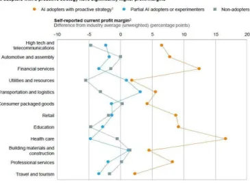
Showing the impact that the adoption of artificial intelligence could have on profit margins, a study conducted by McKinsey & Company (Columbus, 2017) and demonstrates that companies who fully supported AI initiatives have achieved 3 to 15% percentage point higher profit margin, around 12% in the financial industry as shown in the figure 1. Over the 3,000

business leaders who were interviewed for their survey, the majority expect margins to increase by up to 5% points in the next year.

Figure 1: AI Adopters Segmentation (Columbus, 2017)

Corroborating the observations made by McKinsey, Knut Opdal, Rikard Bohm and Thomas Hill (Knut et al., 2017) conducted a research discussing “whether machine learning and automatic hyperparameter optimization represent disruptive technologies for risk management”. Their experiment shows that using a Random Forest instead of a Logistic Regression could lead to an 8% rise of expected profit.

However, while more and more researchers are exploring the use of machine learning and its benefits for credit scoring, banks and credit institutions are making very cautious steps toward its adoption. Thus, the ongoing domination of Logistic Regression in these industries.

As reported in an article from American Banker called “Is AI making credit scores better, or more confusing?” (Crosman, 2017) and as shown in the figure 2 below, if new technology can potentially bring more statistical performance and new lending opportunities, they might also bring more opacity to the credit scoring process and negatively impact the entire credit financial cycle that was built around it.

1.3 “Black Box” Dilemma

One of the most attractive features of new machine learning tools is that it is intended to solve problems that simpler algorithm can’t. The improvement on that aspect could open new market opportunities through the use of new data sources. However, the use of these techniques comes at cost inherent to their functioning, commonly defined as being a “Black Box” (Guidotti et al., 2018).

The term “Black Box” comes from the fact that models created through the process of ensemble models are very complex and their intricate functions cannot be understood by humans. Although practitioners may have a general understanding of the internal flow of an algorithm, the exact path to the output decisions, that may be based on thousands of rules, remain unexplained (Hara & Hayashi, 2016).

While this might not be a significant issue for other industries, the credit system is generally greatly “constrained” by validation, monitoring, reporting and regulations processes that should be considered when using a given modeling tool. As an example, credit scores must usually (at the very least) come with some sort of verbal or written explanation as mandated by the General Data Protection Regulation (GDPR), which theoretically grants citizens a “right to an explanation” in the event that an automated (machine learning based) decision could “significantly affect” them. Thus, the use of a scoring equation that is totally opaque and unexplainable could go against some basic citizens’ Rights (Wachter et al., 2017; Doshi-Velez & Kim, 2017). In this context, a simpler, interpretable models2 _{such as decision trees, rules (Letham}

et al., 2015) or linear models (Ustun & Rudin, 2015) will be preferred even if they don’t have the most predictive performance (Ribeiro et al., 2016).

Recently, Zachary C. Lipton (2018) tried to identify the rationale behind the interest in studying models’ interpretability. It is one of the rare papers to mention, among other field, the interest of interpretability in credit scoring. He points out the fact that “According to their own technical report, FICO trains credit models using logistic regression, specifically citing interpretability as a motivation for the choice of model” (Lipton, 2017).

While the prevailing solution to the issue of the Black Box is to use interpretable models at the cost of lower accuracy (Bastani et al., 2018), research on the topic has been growing rapidly

in recent years3 _{and new methods for complex model decision approximation have emerged}

(Gilpin et al., 2018).

Most of these alternative approaches are all based on the principle of being model-agnostic, so that they can be applied to any decision system. These techniques can involve the superposition of a simple model on top of a Black Box (Craven & Shavlik, 1996) or the perturbations of the original input and analysis of how it impacts the output (Fong & Vedaldi, 2017).

In August 2016, Marco Tulio Ribeiro et al (Ribeiro et al., 2016) heavily contributed to the development of surrogate4 _{interpretation by introducing LIME (Local Interpretable}

Model-Agnostic Explanation); “a novel explanation technique that explains the predictions of any classifier in an interpretable and faithful manner, by learning an interpretable model locally around the prediction”. By assuming that although a complex model might not be simple (or linear) at a global decision level, local region of the decision space might happen to be simple. Consequently, making it possible to fit a simpler model for a specific input region and being able to explain a set of predictions locally. The experiments they’ve made presented evidence that LIME technology can be used in a variety of models in the text and image domains.

In 1996, Mark W. Craven and Jude W. Shavlik (Craven & Shavlik, 1996) presented a method for extracting Tree-Structured representations of trained networks. Their method is similar to LIME technology, but it is specific to neural networks algorithm, as they are approximating simple decision trees to different vectors of the network.

Similarly, Sameer Singh (Singh et al., 2016) proposed to approximate the model locally by using what they call “programs”. A “program” is a set of basic, human friendly set of syntax (“OR”, “AND”, “IF”, “ABOVE”, “BELOW”, “EQUAL”) that are combined with variable for explaining different region of the output space. The method they proposed is highly expressive and can be understood by any human.

Another conceptual framework for approximating a model decision output is through data perturbation. By perturbing the input data and analyze the impact it has on the final output, many practitioners were able to significantly increase their understanding of the model.

In the literature, one can find numerous examples of complex algorithm being better understood with the help of Partial Dependence Plots (PDP), a perturbation base interpretation method introduced by Friedman in 2001 (Friedman, 2001). By plotting the change in predictions of instances as a given feature(s) is perturbed, Green and Kern (2010) were able to understand

3 _{Google Scholar finds more than 20,000 publications related to interpretability in ML in the last five}

years (Doshi-Velez & Kim, 2017).

how the conditional average treatment effect of a voter mobilization is impacted by each variable. In a different context, Elith (Elith et al., 2008) used PDPs to understand how different environmental factors can influence the distribution of a particular freshwater eel while using a gradient boosting.

By inspecting the results of the PDP, Qingyuan Zhao and Trevor Hastie (Zhao & Hastie, 2017) were able to extract causal information from their model. Doing so, they insist on the fact that some domain specific knowledge (business knowledge) is a necessary condition to be applied with the use of PDP method.

In 2017, Ruth C. Fong and A. Vedaldi proposed a “comprehensive, formal framework for learning explanations as meta-predictors” (Fong & Vedaldi, 2017). By perturbing the input of an image classification algorithm, they managed to understand which part of the image contributed the most to the final prediction.

Another type of perturbation was introduced a few years later, this one based on coalitional game theory5 _{(Minhai, 2017) and on the Shapley value. The main idea is to decompose}

the changes in prediction when a set of given value are “ignored”, meaning they are not included in the model. Results tend to demonstrate that the method is efficient and that the explanations are “intuitive and useful” (Strumbelj & Kononenko, 2010). Using a very similar method, Jianbo Chen (Chen et al., 2018) demonstrate that either on language and image data this method compares favorably with other methods using both quantitative metrics and human evaluation.

In 2016, the Shapley Value was further studied by Lundberg (Lundberg, 2016) that created an open source framework (available on Python) for using this new tool. As for as we know, no literature explicitly tested the use of their implementation. In the methodology section (see Shap section) we’ll investigate its current implementation and we will be discussing its outputs on our test use case in the result discussion section of this work.

1.4 Properties of Interpretations

While studying previous literature about model interpretability, we noticed that although many approaches were developed, there is no consensus about a clear definition or technical meaning of what an explanation is (Lipton, 2017).

As a very general ground rule, we could safely state that interpretability is most often associated with the capacity of a human to understand the cause of a decision (Gilpin et al., 2018 – Miller, 2019 - Kim et al., 2016), but the practical form it takes e.g., completeness, compactness

or comprehensibility, remain mostly subjective to each work (Guidotti et al., 2018). Even in the scope of GDPR, there is no information about the expected properties of required explanation (Rudin, 2018).

For each studied paper, it seems that authors are usually adapting their technical expectations of the interpretation according to the field of their work (e.g., image recognition, medicine …) or to the method they are implementing. On this matter, it seems legitimate to imagine that different technical representations of Black Box’ explanations could be appropriate for different kinds of users and fields of application (Singh et al., 2016).

In that context, a distinction which we believe fundamental has nonetheless started to emerge. An interpretation method can be considered as being Local or Global level (Guidotti et al., 2018). Although most literature reviewed only implicitly specify if their proposal is global or local, we try to give an overview of the distinction of both as it strongly impact the methodology of our work.

● Global Interpretation

Interpreting a model globally means representing the internal functioning of a trained model in a human understandable way (Yang et al., 2018). It is usually done by an aggregation of instance explanations over many (training) instances (Robnik-Sikonja, 2017) or by simply reading the model’s output (linear models). Global interpretation of complex algorithms is known to be either not possible, or too simplistic to represent the original model, thus, the recent development of tools (local surrogate models) to interpret the model locally (Ribeiro et al., 2016).

● Local Explanation

Interpreting a model locally means that you can focus on a single instance and examine what the model predicts for this specific input, and explain why (Molnar, 2019). It usually comes with providing the impact of input feature values on the prediction (Robnik-Sikonja, 2017)

Despite the soaring attention to the topic, the general conceptual framework of model interpretability has not been defined. Consequently, it is still hard for any business or practitioner to rely on such technologies since we can hardly set expectation regarding their uses, thus making difficult to understand its potential benefits.

1.5 Motivations and Methodology

In this work, we first intend to demonstrate the benefits of using a complex Black Box model over a standard Logistic Regression Scorecard by comparing it using state of the art statistical performance metrics. In a second time, we try to understand if the use of two

interpretation techniques, namely Partial Dependence Plots and Shapley Additive Explanation could help in understanding the functioning of a specific complex model.

By applying these methods in the specific field of Credit Scoring, we hope to contribute to a better understanding of what interpretation methods are and what to expect from them in this particular field. The growing interest of using Black Box models and the recent questions around data regulation are opening a new, promising, area of investigation. In that context, we hope that our work could open the way for further empirical studies that are necessary to back up the work being done by a raising community of researchers and practitioners.

Throughout the following paper, we build two statistical models, a Scorecard algorithm, already mentioned, along with a more complex one, considered as a Black Box tool usually referred to as Extreme Gradient Boosting (XGBoost).

The scorecard algorithm was built using James, the flagship product of James startup used by many financial institutions for assessing risks at the time of credit application. The product was embedded with state-of-the-art techniques and is the results of many years of research from the James’ team and its partners within the financial industry.

The XGBoost algorithm, not yet available inside of James, was built in python, using building and optimization techniques that are as close as possible from James, in order to test both models in the same conditions. Given the very recent development of this tool and some of its components that will be used here, this work also opens the way for evaluating its potential applicability in the Credit Scoring context.

Before to analyze the results of each algorithm in the Results and Discussion section of this document, we will first provide the reader with contextual information about the data that is going to be used and its preprocessing. We will then cover the basic theoretical knowledge that we believe necessary to understand both the current implementation of the Scorecard in the Credit industry and the functioning of the XGBoost model. Some basic knowledge will be given about the way the model hyper parameters optimization is done within James (and reproduced in Python) without getting in much details since it is not the scope of our research.

Finally, we will define the evaluation and interpretation metrics that will be used for evaluating our two models, necessary step before to jump into the actual evaluation and interpretation of both algorithms.

2 Data Description and Cleansing

It is not uncommon to find the expression “Garbage in, garbage out” when reading about predictive modelling. This expression shows the importance of having relevant data in its best shape in order to be possible to construct a good model.

2.1 Data Discovery

The data used in this project comes from the competition "Give me some credit" launched on the website Kaggle. It consists of 150,000 consumers, each characterized by the 10 variables described in the table below.

Variable

Description

Type

Serious Delinquency 2 years Person experienced 90 days past due delinquency or worse within 2 years Y/N

Revolving Utilization of Unsecured Lines

Total balance on credit cards and personal lines of credit except real estate and no installment debt like car loans divided by

the sum of credit limits percentage

Age Age of borrower in years integer

Number of Time 30-59 Days Past Due Not Worse

Number of times borrower has been 30-59 days past due but no worse in the last 2

years. integer

Debt Ratio Monthly debt payments, alimony, living costs divided by monthly gross income percentage

Monthly Income Monthly income real

Number of Open Credit Lines and Loans

Number of Open loans (installment like car loan or mortgage) and Lines of credit (e.g.,

credit cards) integer

Number of Times 90 Days Late Number of times borrower has been 90 days or more past due. integer

Number Real Estate Loans or Lines Number of mortgage and real estate loans including home equity lines of credit integer

Number of Time 60-89 Days Past Due Not Worse

Number of times borrower has been 60-89 days past due but no worse in the last 2

years. integer

Number of Dependents Number of dependents in family excluding themselves (spouse, children etc.) integer

Table 1 Data Dictionary

As described in the table above, the event that we will be trying to predict is given by the Serious Delinquency 2 years variable. It indicates if the person that was granted a loan experienced 90 days past due delinquency or worse in the 2 years after receiving the loan. Equally said, it is an indication of 3 consecutive months without payment the installment. In the data, it is coded as “1” if the event occurred and “0” otherwise. By calculating some basic proportion statistics, we get the table below:

SeriousDlqin2yrs Count Rates

< 90 days past due 139974 93,32%

> 90 days past due 10026 6,68%

Table 2 : Default Rate Analysis

As one can see, the proportion of people that experience 90 days past due is 6.68%, which represent 10,026 cases.

Some basic descriptive statistics of the rest of the variable is given in the table below.

mean Standard Deviation min Quantile25% Median Quantile75% max

Revolving Utilization of

Unsecured Lines 5.90 257.04 0.00 0.04 0.18 0.58 50708

Age 51.29 14.43 0 40 51 61 103

Number of Time 30-59 Days Past

Due Not Worse 0.38 3.50 0 0 0 0 98

Debt Ratio 26.60 424.45 0 0.14 0.30 0.48 61106

Monthly Income 6670 14384 0 3400 5400 8249 3008750

Number of Open Credit Lines

and Loans 8.76 5.17 0 5 8 11 58

Number of Times 90 Days Late 0.21 3.47 0 0 0 0 98

Number Real Estate Loans or

Lines 01.05 1.15 0 0 1 2 54

Number of Time 0-89 Days Past

Due Not Worse 0.19 3.45 0 0 0 0 98

Number of Dependents 0.85 1.15 0 0 0 2 20

Table 3 : Descriptive Statistics

As one can observe, we can see some inconsistencies in the data by looking at this table. For example, we see that the minimum age is “0” (zero) which does not make sense in the context of credit application. In a later section, we’ll go through each variable, study their distribution and clean intervene in such inconsistencies as the one for Age variable.

2.2 Missing Values

Missing data arise in almost all serious statistical analyses. Since most statistical models and machine learning algorithms rely on a data sets that is free of missing values, it is of a major importance to handle the missing data appropriately. Simple methods may suffice sometime in some case (imputation with the mean or omission of the instances with missings). Some algorithm like CART naturally account for missing data and there is no need for imputation (Wagstaff, 2004). In many other situations, missing values should be imputed prior to running statistical analyses.

We can observe in the table below the number of missing and the percentage of instances it represents for each variable in our original dataset.

Variable

Number of

Missings

% of Missings

Serious Dlqin 2 yrs 0 0,00%

Revolving Utilization of Unsecured Lines 0 0,00%

Age 0 0,00%

Number of Time 30-59 Days Past Due Not Worse 0 0,00%

Debt Ratio 0 0,00%

Monthly Income 29 731 19,82%

Number of Open Credit Lines and Loans 0 0,00%

Number of Times 90 Days Late 0 0,00%

Number Real Estate Loans or Lines 0 0,00%

Number of Time 60-89 Days Past Due Not Worse 0 0,00%

Number of Dependents 3 924 2,62%

Table 4 : Missing Values

With 29,731 missings (≅20% of missing value) for the Monthly Income, imputing with a standard technique such as the mean or the median might significantly affect the distribution of the variable. Doing so, there is a risk that the learning of an algorithm would end up being biased in some way (if not treated specifically for this algorithm). For this reason, the 29,731 instances with missings were removed from the data. Doing so, all the missings from the Number of Dependents variable were also removed in the process.

We finally ended up with a clean (no missing values) dataset consisting of 120, 269 instances.

2.3 Outliers

Before to go through each variable for which potential outliers were detected in our case, it is important to highlight the specificity of the 2 algorithms that we will explain and use. Each type of algorithm deals differently with outlier and may require special preprocessing.

For the scorecard algorithm, all the continuous variables will be bucketed, i.e. variables are categorized into logical intervals, for ease of interpretation and implementation. This truncation that is usually used in credit scoring is known for significantly reducing the effect and influence of outliers/ extreme values (Bolton, 2010).

Regarding the XGBoost algorithm, it is an ensemble model based on CART6_{, which is}

known to be extremely resistant to outliers (up to a certain number) (Sutton, 2005).

Due to the points above, our strategy for the treatment of outlier will be:

● Removal of outlier if they represent a too significant number of instances (limit of 1,000);

● Imputation with the median of the same variable if it represents a low number of instances and that the value is obviously not possible (a negative income for example);

● No action if the extreme nature of the value is doubtful and if it represents a low number of instances.

Age

Figure 3: Age Distribution

As one can observe, the Age variable is ranging from 0 to 100. But to be qualified as a borrower, the person must be at least 18 years. There were one only record with a value of “0”, obviously being an outlier. Hence, we imputed this instance with the median age (51 years old).

Debt Ratio

Figure 4: Debt Ratio Distribution

Although a Debt Ratio may exceptionally be higher than 1 (100%), we identified 2,106 cases that had a value over 10 (1000%). Such a significant number might result in affecting the learning of the algorithm, so we decided to remove those instances. After doing so, the new dataset consists in 118,163 instances.

Number of Dependents

Figure 5: Number of Dependents Distribution

In that case, we identified 11 cases for which the Number of Dependents was above 8. Although it may be the result of an error in the application form or from other source, it is a hard statement to make because the maximum is not so far from the end of the distribution plot. Also, we considered that the algorithm should be robust to such a low number of concerned instances and that any kind of treatment was not necessary.

Number of Times 90 Days Late

Figure 6: Number of Times 90 Days Late Distribution

For this variable, we identified 148 cases for which the Number of Time 90 Days Late was above 20. We considered that the algorithm should be robust to such a low number of concerned instances.

Monthly Income

Figure 7: Monthly Income Distribution

For the Monthly Income, we identified 300 cases above 50,000. We considered that the algorithm should be robust to such a low number of concerned instances.

Revolving Utilization of Unsecured Lines

Figure 8: Revolving Utilization of Unsecured Lines Distribution

In this case, we found it weird to be above 1 (100%) because credit card usually have a limit that we cannot overpass (possible for some payments so extra fees can add up). On the graph above, we can observe an abrupt fall in the distribution after 1. We identified 2,773 cases above 100% and removed them from the analysis since it could affect the algorithm.

3 Variable Selection and Data Partitioning

The transformed variables were assessed in terms of their power in discriminating between “good” and “bad” clients. In order to do that, statistic indicator Univariate GINI was used.

3.1 Univariate GINI index

GINI index is a measure for quantifying the ability of a numeric feature to distinguish between classes (Zhao et al., 2010). It is used by many practitioners as a feature evaluation and selection tool. It has shown to be quite performant in many domains as it can significantly improve the learning performance compared to several existing feature selection criterions (Singh et al., 2010 - Liu et al., 2010)

Index

Variable

Univariate

GINI

0 Revolving Utilization of Unsecured Lines 0,496

1 Number of Time 30-59 Days Past Due Not Worse 0,348

2 Number of Times 90 Days Late 0,282

3 Age -0,227

4 Number of Time 60-89 Days Past Due Not Worse 0,216

5 Monthly Income -0,152

6 Debt Ratio 0,14

7 Number of Dependents 0,093

8 Number of Open Credit Lines and Loans -0,064

9 Number Real Estate Loans or Lines -0,049

Table 5 : Univariate GINI

As shown in the table 5 above, Revolving Utilization of Unsecured Lines variable is showing the more importance in term of Univariate GINI. As a credit risk analyst, we would expect a high and frequent utilization of the credit limit to be an important vector of risk since it may be a symptom of a particular behavior of not managing well debts and monthly payments.

The importance of 30-59 and 90 days past due is easy to interpret as they describe a past state of delinquency, as the one we are trying to predict (90 days late). It is interesting to note that 60-89 days past due has a relatively lower importance while it represents a very similar behavior.

Any of the independent variables (predictor) that would potentially be included in the model cannot be highly correlated with another variable. If so, the accuracy and stability model we will build might be compromised.

Therefore, a correlation assessment was performed using the Pearson coefficient which is a measure of the strength of a linear association between two variables. This correlation metric attempts to draw a line that best fit through the data points of two variables by reducing as much as possible the distance between the points and the line. The Pearson correlation coefficient is a generalization of these distance of all points from the line.

In case of having highly correlated variables (above 30% correlation), we removed one of the correlated variables based on two conditions:

1) The potential discriminatory power (Univariate GINI statistic) of the two variables

2) Business/human (intuitive) considerations

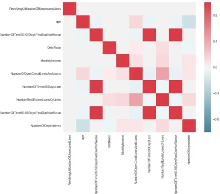
The figure 9 below gives a visual illustration of all the correlation of our dataset.

Figure 9: Correlation between 10 variables (Numeric table in annex nº2)

Having a look at the correlation table, we can identify 6 variables that have at least a correlation above 30%. Namely;

- Number of Time 30-59 Days Past Due Not Worse, - Number of Time 60-89 Days Past Due Not Worse,

- Number of Times 90 Days Late, - Number of Dependents,

- Number of Open Credit Lines and Loans, - Age.

In the list above, the variables that were finally removed were highlighted in red for better visualization purposes, for each one of them, the rationale is explained below.

Number Real Estate Loans or Lines and Number of Open Credit Lines and Loans variables are showing a correlation of 43%. For this pair, Number Real Estate Loans or Lines variable was removed because it has a lower Univariate GINI (-0.08 against -0.07). As one could expect, Number of Time 30-59 Days Past Due Not Worse, Number of Time 60-89 Days Past Due Not Worse and Number of Times 90 Days Late are cross-correlated above 98%.

We chose to keep Number of Times 90 Days Late variable although it didn’t have the highest Univariate GINI because it is the one that is the closest from the target in term of business definition. Compared with the two others, Number of Time 60-89 Days Past Due Not Worse variable the lowest Univariate GINI.

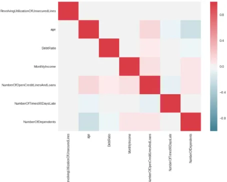
The new correlation table after removing the three aforementioned is presented in the figure 10 below. In this final set of variables, the maximum correlation is 21% (between Age and Number of Dependents)

3.3 Sampling: Model Training and Testing

Model validation is primarily a way of measuring the predictive reliability of a statistical model and keep control of the learning procedure. The basic idea is to use part of the dataset to train the classifier (train set) and another part of the data to test the classifier (test set) as if it was “new data”. The aim is to maximize the accuracy of the model (bias) while minimizing its complexity (variance).

The holdout method is a very simple kind of model validation method and is one of the most commonly used. It consists in separating the data into two sets usually referred as the training set and the test set (see figure 11 below). The algorithm will be ran looking only at the training set and we use the test set to evaluate its performance.

Figure 11: Holdout Train Test Split

This validation method is known to lead to a low accuracy (bias or overfitting) since the evaluation heavily depends on how the data points are distributed between the training and the test. Therefore, the final evaluation may differ depending on the data distribution, leading to a poor generalization with new “unseen” data.

According to many studies, the traditional approach for tackling this bias or overfitting problem is k-fold cross-validation (Kim, 2009). This method, embedded within James product, is a generalization of the hold out method in which meanwhile the data set is randomly partitioned into K subsets, each subset is used as a test set, considering the other K-1 subsets as training set (Witten et al., 2016). In this approach, the entire dataset is used for both training and testing the model. Typically, a value of K=10 is used in the literature (Mitchell, 2017).

In our specific case, we will follow the specification of the model validation made in James, detailed below and illustrated in the figure nº12 below.

James tool is using a combination of the two methods mentioned above, that is, after splitting the data set into train and test set, the training set is again split into 3 validation sets for the fitting of the algorithm.

Figure 12: Validation and testing methodology

As no date variable was part of the data provided, we used a stratified random sampling method for partitioning the data between the train and the test set of the holdout method. The stratify method allow to keep the same default rate between the train and the test set. A splitting configuration of 20% of the data allocated to the test set was chosen.

4 Modelling Techniques

4.1 Scorecard

4.1.1 Logistic Regression

While a lot of different models can come to mind when talking about linear models, we will focus our attention on linear and a derivation of it, Logistic Regression.

As for any predictive algorithm, the main goal of a Linear Regression is to generalize an event using characteristics that we assume to be a partial description of a wider phenomenon. In our case, we want our model to estimate a probability of a 90 Days Past Due Or Worse happening or not during the credit lifetime.

In the case of linear regression, the interaction between different predictors and a target response or event is represented by a straight line that will become the estimated predictor for each data observation. The shape and the slope of this line is defined by a set of parameters minimizing the mean squared error (average distance between the estimated predictor and the actual value to be estimated). The parameters of the Linear Regression are defined by the formula:

" = %_& + %₍) + *

%₊ is the intercept (5 on the graphic below) and %₍ is the slope of the red line. The figure 13 below represents the observations (blue dots) and the regression line (red line) on a (), ") axis, X being a single predictor and Y a continuous Target.

Figure 13: Linear Regression

In the case of credit scoring, the event we are trying to predict is binary. Drawing a line to represent its relationship with another characteristic would therefore not make much sense. In fact, using a Linear Regression to predict this type of dependent variable would be violating several mathematical assumptions inherent to the concepts that defines the Linear Regression. A

visual illustration of the problem is given by the figure 14 below, where 2 possible outcomes (1 or 0) of an event " are associated with a characteristic ):

Figure 14: Binary Problem Representation

To resolve this dilemma, we should assume that the probability law that defines the probability of " being 1 given the characteristics of an individual (otherwise written /(" = 1 | ) = 2)) is Logistic. The Logistic Regression is therefore assumed to be following a logistic law defined by the cumulative distribution function:

3(2) = 1

1 + 42567

By looking at the figure 15, one can observe that the " axis is no longer defined by the dependent variable but by the probability of this dependent variable to be equal to 1 (it would be the probability that a customer defaults in credit scoring).

.

Figure 15: Logistic Regression

When fitting a Logistic Regression, we try to find the optimal parameters values that will be associated with one or several predictors. Those parameters are usually optimized toward the maximization of the likelihood7 _{of the event " happening or not.}

For the sake of illustration, we will consider that we only have two predictors )₍ and )₈. The model is therefore:

7 _{Maximum likelihood estimation is a method that determines values for the parameters of a model. The}

parameter values are set in a way that the produced output of the model is as close as possible from the event that is actually observed.

/(" = 1 | )) = 1

1 + 4256(9: ; 9<=<; 9>=>)

With this function, we then estimate %_&, and %₍ and %₈ (with likelihood maximisation) and define the decision boundary of the model.

For model interpretation purposes, it is important to point out that the final values of each Beta is a constant measure of change of the logit transformed probability of Y for one unit change in the input variable. The equation for the logit transformation of a probability of an event is given by:

?@ABC (5D) = %&+ %()(+. . . +%F)F

where 5 is the posterior probability of the event, ) are input variables, %& is the intercept of the

regression line and %F are the parameters associated with each variable.

The logit transformation can be interpreted as the log of the odds, that is, G@A( H(IJIKL)

H(KMK IJIKL)). It is used to linearize posterior probability and limit outcome of estimated

probabilities in the model between 0 and 1. By selecting a cutoff out of the logit transformed probabilities given by the Logistic Regression, we are then able to classify each observation into the class 1 or 0. This is why the Logistic Regression is often referred to as a linear classifier.

As a parametric method, the Logistic Regression is not free from several critics, mainly residing in the assumptions it takes such as:

● linear relationship; ● independent error terms; ● uncorrelated predictors; ● use of relevant variables.

These assumptions (like the linear relationship), when violated, naturally compromise the model accuracy. The limited complexity associated to the Logistic Regression is the main disadvantage in comparison to other (non-parametric) techniques. On the other hand, it has advantages compared to this later group of methods such as having results that are easy to interpret (due to the log constant scaling) and usually requiring less data.

4.1.2 Scorecard

A Credit Scorecard can be defined as a mathematical procedure that tries to estimate the likelihood of a customer to display a particular behavior (to be in default for example).

This predictive procedure can be based on any model but the most common way to go is to use a Logistic Regression (Anderson, 2007).

The output of the scorecard is a score that can take different range (e.g., 200 - 800). A customer having a low score would be considered at risk of displaying the event we’re trying to predict (to be in default for example). On the other hand, a high score indicated a low chance of displaying the given event.

The overall score of an individual is calculated from a scorecard table in which a number of “points” are associated with different characteristics that were used in the model. All those “points” are aggregated for each individual in order to obtain their final score. (Anderson, 2007) An example of such a table is given below in the figure 16.

Figure 16: Example Scorecard (Anderson, 2007)

At first sight, it might be hard to understand the relationship between the table presented above and the Logistic Regression explained in the previous section of this work.

To get an accurate intuition about this, we need to go a step before the modelling phase and focus our attention on how the data was prepared before the training of the Logistic Regression. Indeed, the construction of a scorecard involved the careful binning8 _{of every}

numerical variable. Doing this, each observation of a data set is no longer represented by the actual value of its attributes but by its affiliation to a range

of value (for numerical variables).

The comprehension of the client portfolio might indeed impact the way the ranges should be created. One might want to create groups that respects operational and business considerations

(using some strategy in grouping postal codes or choosing defined ranges to coincide with corporate policies for example) (Siddiqi, 2017).

To make sure that, during the binning process, each group we create is somehow differentiable from other groups (in term of default rate as an example), the weight of evidence (WOE) of the different categories are examined and grouped together if they have similar relative risk (if the WOE is similar).

The Weight of Evidence is a heavily used measure in credit scoring for assessing the "strength” of a grouping (

Garla, 2013

NOP_D = GQ(( RD S_{D T (}K _R D)/( /_D S_{D T (}K _/ D))

where / is the number of occurrences (default), R is the number of non-occurrences (non-default) and B the index of the attribute being evaluated. A precondition for the calculation is non-zero values for all R_D and /_D .

The WOE does not consider the proportion of observations, so it measures a relative risk, given the overall event rate (default rate). A negative WoE indicates that the proportion of defaults is higher for that attribute than the overall proportion and indicates higher risk. By nature, the weight of Evidence is also commonly used for feature selection, since having a binned variable with very disparate WoE for each group indicate that this predictor is strong in differentiating goods from “Bads”.

However, the statistical strength is not the only factor to take into account for considering a variable as a meaningful predictor.

In the figure nº 17 presented below, one can observe an example of a binning procedure on Age variable.

Figure 17: Binning of Age Variable (Anderson, 2007)

Missings information are always grouped together as a separate group as shown on the left part of the graph (Zeng, 2014).

By looking at this simple line, we can see that population ranging between 23-26 and 30-44 years old have a very strong relative rate of event (default rate). On the other hand, 35-30-44 years

old ranging population is relatively less exposed to the event occurrence (default). In between, we observe strong reversals that, in a lot of cases, might be going against business experience or operational considerations. In the example above, a lot of decision makers would be expecting a linear relationship between the Age and the risk.

Applying a Logistic Regression on the example above (without adjusting the bins) would potentially lead to the attribution of more “credit points” (less risk) to 18-22 years old population than for the 30-35 years old one. In between, the opposite trend is observed between younger and older (23-26 years old would be granted less points than 27-29 years old). If not backed up by strong evidence and acceptable explanation, this decision-making strategy would be very hard to be considered as logic and fair.

An example of logical trend is presented in the figure 18 below. In this case, the allocation of risk (and mechanically, of the “points” that will be attributed to each group) is having a linear and logical relationship between the attributes in Age and proportion of “Bads”. This trend would much likely confirm the intuition and business experience of decision makers.

Figure 18: WoE and Logical Trends (Anderson, 2007)

In some cases, however, reversals may be reflecting actual behavior (“U” shaped pattern for example) and masking them may decrease the overall strength of the predictor. As already mentioned, this type of behavior should be investigated first, to see if there is a valid business explanation behind

Given the lack of business knowledge due to the external source of the data, the above process was purely based on a statistical approach, establishing relationships with the only objective of ensuring logical trend.

Due to obvious mathematical reasons, in some cases, reaching a logical trend might be mechanically impossible without drastically reducing the number of bins. This is why some variables had to be reduced to the minimum possible bucketing number of two. The full table with results of binning process for all the variable can be found in the annex nº1.

After the binning is performed, the next step to follow is to encode each bin with its associated WoE. This way the variable will shift from a categorical to a numerical type while conserving its linear trend (high WoE bins will be ordinally higher than lower ones).

Using the table nº 6 presented below for age, each data points of the variable will be encoded with the respective WoE of the bucket in which it falls into (-0.478 for a data point of 3 years old for example).

age

COUNT

WOE

[21, 35.5] 13771 -0,478 (35.5, 42.5] 12848 -0,271 (42.5, 50.5] 18739 -0,161 (50.5, 57.5] 15581 -0,021 (57.5, 63.5] 12369 0,369 (63.5, 103] 19032 0,898

Table 6 : Age Variable Final Encoding

This recoding of predictors is particularly well suited for subsequent modeling using Logistic Regression. By fitting a linear regression equation of predictors (encoded with WoE) to predict the logit-transformed binary Y variable, the predictors are all prepared and coded to the same (WoE) scale, and the parameters in the linear logistic regression equation can be fairly compared.

After fitting the logistic regression, the output of the algorithm can be scaled in many formats. In some cases (depending on implementation platforms, regulatory requirements or other factors) the scorecard has to be produced in a specific format. In this case, a scaling parameterization needs to be applied.

Scaling refers to the range and format of scores in a scorecard and the rate of change in odds for increases in score. The score is usually defined as the good/bad odd (e.g., score of 8 means a 8:1 odd -- equivalent to 8% chance of event or default) and it can have very specific shape defined for example by:

● the definition of a numerical minimum or maximum scale (e.g., 0–1000 or 300– 800);

● the definition of a specific odds ratio at a given point (e.g., odds of 5:1 at 500); ● the definition of a specific rate of change of the odds (e.g., double every 50

points).

Since the choice of scaling does not impact the predictive power of the model, it is a decision that is only based on operational or regulatory considerations (Siddiqi, 2017).

4.2 XGBoost

Since 2015, a first to try, always winning Non-Parametric algorithm surged to the surface: XGBoost. This algorithm re-implements the tree boosting and gained popularity by winning Kaggle and other data science competition (Nielsen, 2016). XGBoost is able to solve real world scale problems using a minimal amount of resources (Chen & Guestrin, 2016).

In this section, we will introduce all the basic techniques that are implemented in the XGBoost that we are using in our work. We will take a try to understand the theoretical background needed for the understanding of the XGBoost, going through CART Decision Trees, Ensemble Models and boosting techniques.

4.2.1 CART - Decision Tree

Decision trees are another classification technique used for developing credit scoring models, also known as recursive partitioning (Hand & Henley, 1997), Additive Tree Model (ATMs) (Cui et al., 2015) or Classification and Regression Trees (CART).

These types of algorithm are important in the machine learning community since it have been around for decades and modern variations like Random Forest are among the most powerful techniques available.

Used within XGBoost (XGBoost Documentation), a CART decision tree is a simple model that tries to predict the value of a target event by inferring simple decision rules from the training data. In other words, a decision tree is a set of rules used to classify data into categories (Good vs Bad or default vs non-default).

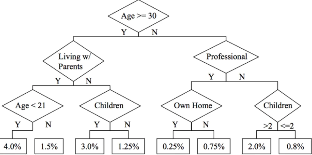
The top of the tree as shown above contains the full training data and is referred as the root node. Each inferior stage of the tree level is referred as child nodes, and at the bottom, we have the terminal nodes. The depth of tree, (the number of levels it can build) are among the parameters that are defined by the user. If no limit was set, the algorithm would split the data until it can reach a terminal node that is completely pure (containing only “Bad” or only “Good”). At the end, the terminal node values can be used as estimates (scores), or as a grouping tool. In our case (binary outcome), the value given by the terminal node is a probability.

There are several possible splitting criterions in decision trees for building these rules. Entropy is one of them (used in XGBoost) and it is the one we will present here. Two kinds of entropy must be calculated at each branch level of the decision tree in order to perform the split:

1. The Set entropy: looking at the whole data set, it defines the number of individuals in each class and calculate 5_D (percentage of total individuals in class B) and then the target entropy. It is defined by:

PQCX@5] (V4C) = − _ /(`[Ga4<sub>D</sub>). G@A<sub>8</sub>(/(`[Ga4_D))

F

DT(

where \ is the number of classes (two in our case: safe and default).

2. Each Feature entropy: it is the same principle as for the set entropy but with a different method of calculation. For each feature N, we use its frequency table. The formula is defined by: PQCX@5] (34[CaX4) = _( Rº @Y BQ\B`B\a[GZ BQ WℎBG\ Q@\4 B Rº @Y C@C[G BQ\B`B\a[GZ @Q Cℎ4 5[X4QC Q@\4) K DT( . PQCX@5](WℎBG\ Q@\4 B) The information gain is then calculated for each splitting option of each feature. This metric measures the reduction in entropy that we get from the splitting of a given feature and splitting border. It is defined by:

d[BQ(V4C, 34[CaX4) = PQCX@5] (V4C) − PQCX@5] (34[CaX4)

Thus, after assessing all the features, the one that maximizes the reduction in entropy (with the largest information gain) is the chosen one to perform the split. With new data, the algorithm will apply the previously defined set of rules to the new observations. At the end of the process, each instance will end up in a specific endpoint and assigned a predicted class.

In the literature and empirical evaluation studies, Decision trees are usually considered as a powerful analysis tools since it allows the discovering of feature interactions toward the

explanation of a specific event. However, it usually provides poor results and require an important amount of data in order to be significant (Anderson, 2007).

4.2.2 Ensemble Models

The ensemble method consists in the idea that a set of individually trained weak classifiers or learners (such as decision trees), performing weakly alone, can be combined to become better by reducing the prediction errors (Buja & Stuetzle, 2006). Previous research has shown that an ensemble is generally more accurate than any of the single classifiers in the ensemble, especially when it comes to decision trees (Opitz, 1999).

Two popular methods for creating accurate ensembles are Bagging (Breiman, 1996) and Boosting (Freund & Schapire, 1996). These methods usually rely on “resampling” techniques to obtain different training sets for each of the individual classifiers. Each tree is grown using CART methodology described earlier (Breiman et al., 1984).

Bagging (Breiman, 1996), also known as “bootstrap” (Efron & Tibshirani, 1993) ensemble method is based on the statistical concept of estimating quantities about a population by averaging estimates from multiple subsets of data samples. Breiman was the first to present empirical evidence that bagging can significantly reduce prediction error (or variance) of the algorithm. Applied to machine learning, the bagging consists in creating a random subset of instances and in a redistribution of the training set for each individual classifier that compose the ensemble.

In many ensemble approaches such as Random Forest, each tree is also built by selecting at random a small group of input coordinates (also called features or predictors) to be included in each individual learner. In the end, a chosen metric (e.g., Majority-Voting) is calculating the proportion of trees that classified one individual in each class and the class with the biggest importance defines the predicted class membership as shown in the illustration below (figure 20).

As an ensemble decision tree model, XGBoost is based on the second ensemble prediction method mention earlier as boosting. Brought by Jérôme Friedman, this technique produces competitive, highly robust predictions for both regression and classification (Friedman, 2001)

The idea of the boosting methods is to produce individual classifiers sequentially and not randomly as it is done with bagging. To do so, the subset of training data used for each member of the ensemble is chosen based on the performance of the classifier(s) built previously during the construction of the ensemble. More specifically, examples that are incorrectly predicted by previous classifiers are chosen more often than examples that were correctly predicted. The problematic of ensemble modelling, with the perspective a boosting technique became about whether a weak learner can be modified to become better. Adaboost (Freund & Schapire, 1997), is usually considered to be the first successful example of a boosting algorithm.

In the end of the boosting process, there is M classifiers (M depending on the number of iterations defined by the user). After evaluating the weight of each of tree, based on their error rate, the final classification is made by combining the outputs of all classifier relatively to the weight associated to each one of them and to the chosen averaging method.

4.2.3 Gradient Boosting

Given the success of the Adaboost method, the statistics community developed a generalization of the boosting method applied to arbitrary loss functions: the Gradient Boosting (Friedman, 2001 - Sigrist, 2018).

This method is based on the concept of the gradient descent algorithm which is a first-order iterative optimization algorithm for finding the minimum of a function. This algorithm initiates the optimization of a formula Y(2) with a random value for 2, and performs several iterations using the formula below to update the value.

2_{efggIKL DLIghLDMK} = 2_{igIJDMfj DLIghLDMK} − k l Y (2igIJDMfj DLIghLDMK) l 2igIJDMfj DLIghLDMK

With ᶯ being the magnitude step that will determine the size of the following one. The term that follows is the gradient that gives the direction to be taken for minimizing the loss function.

After initializing a model with a constant value, at each iteration the algorithm computes the pseudo residuals (gradient of the error with respect to the loss predictions of the previous model)according to the following formula:

X_Dm = − n l ? ("D, (2D)

l 3(2_D) o , Y@X B = 1, 2, … , Q

Then, it trains the following tree using this pseudo residuals as a new target to predict. Doing so, each new tree specializes into predicting well the previous instances that were wrongly predicted by trying to minimize the loss function.

In the case of the XGBoost, it actually uses a minimization technique derived from the gradient boosting method known as Newton boosting (Nielsen, 2016 - Chen & Guestrin, 2016 - Sigrist, 2018). As we saw, the Gradient boosting is based on a first-order gradient descent updates while the other is based on a second-order gradient descent update. Recent research tends to show that Newton boosting performs significantly better than the other boosting variants for classification (Sigrist, 2018) as it gives a more accurate view of the direction to take for minimizing the loss function.

5 Hyper-Parameters Optimization

As it is done in James and in many Credit Risk related machine learning task, our study will also include the careful tuning of learning parameters and model hyperparameters. hyperparameters usually refers to model properties that cannot be directly learned from the regular training process. It can be the complexity of the model or how fast it should learn, which are usually fixed before the training or the boosting optimization. The following section aims at giving a brief introduction to hyperparameters optimization problematic and one of its solution, used within James software: Gaussian Process or Bayesian optimization.

5.1 Bayesian optimization

Bayesian optimization has proved to be a good choice in many contexts by yielding to better performance when compared with other state of the art optimization techniques. In theory, it works by assuming that the function to optimize follow a Gaussian process9 _{and keep a posterior}

distribution of this function while results with different hyperparameters are observed (Mockus et al. 2014).

As the number of iterations grows, the posterior distribution of the loss function becomes more accurate and it becomes more clear which regions of the parameter space are should be explored further and which one should not, as shown in the figure 21 below.

Figure 21: Illustration of a Bayesian optimization Process