Fiscal Activism and Price Volatility: Evidence from Advanced and Emerging Economies

(1)

António Afonso,

João Tovar Jalles

Fiscal Activism and Price Volatility:

Evidence from Advanced and Emerging

Economies

WP04/2017/DE/UECE

_________________________________________________________

W

ORKING

P

APERS

(2)

Fiscal Activism and Price Volatility: Evidence

from Advanced and Emerging Economies

*

António Afonso

$

_{João Tovar Jalles}

+

2016

Abstract

Using a panel of 54 countries between 1980 and 2013, we find empirical support for the view that changes in the fiscal policy stance (year-on-year change in the cyclically adjusted primary balance) have a significant positive correlation with inflation volatility. An increase in the volatility of discretionary fiscal policies by one standard deviation raises inflation volatility between 5 and 6 percent. Moreover, results using alternatively different inflation volatility proxies confirm that an expansionary fiscal stance increases price volatility. Another relevant outcome is that in a context of economic expansions (recessions) the harmful impact of fiscal activism on price volatility is soften (heightened), while the negative impact of fiscal activism on price stability is higher when fiscal policy is expansionary. Finally, fiscal activism fuels inflation volatility much more pronouncedly in emerging market economies vis-a-vis advanced economies.

JEL: C23, E31, E62, G01, H62

Keywords: volatility, fiscal policy, inflation, GARCH, Consensus Forecasts

*_{The opinions expressed herein are those of the authors and do not necessarily reflect those of their employers. Any remaining}

errors are the authors’ sole responsibility.

$_{ISEG/ULisbon – University of Lisbon, Department of Economics; UECE – Research Unit on Complexity and Economics, R.}

Miguel Lupi 20, 1249-078 Lisbon, Portugal, email: aafonso@iseg.utl.pt. UECE (Research Unit on Complexity and Economics) is financially supported by FCT (Fundação para a Ciência e a Tecnologia), Portugal. This article is part of the Strategic Project (UID/ECO/00436/2013). email: aafonso@iseg.utl.pt.

+_{Centre for Globalization and Governance, Nova School of Business and Economics, Campus Campolide, Lisbon, 1099-032}

Portugal. UECE – Research Unit on Complexity and Economics, R. Miguel Lupi 20, 1249-078 Lisbon, Portugal. email:

(3)

1. Introduction

Inflation volatility has been an important topic in the literature looking at the relationship

between inflation and economic growth. On the one hand, several studies have concluded that

high inflation (and associated high inflation volatility) are generally harmful to growth. On the

other hand, only few studies have focused on disentangling the individual channels through

which such effect occurs. High variability of inflation over time makes expectations over the

future price level more uncertain. In a world with nominal contracts this induces risk premia for

long-term arrangements, raises costs for hedging against inflation risks and leads to unanticipated

redistribution of wealth. Thus, inflation volatility can impede growth even if inflation on average

remains restrained (Friedman, 1977).

Judson and Orphanides (1999) found evidence that inflation volatility (measured by the

standard deviation of intra-year inflation rates) has led to lower economic growth in a large panel

of countries. Also, Froyen and Waud (1987) found that high inflation induces high inflation

volatility and uncertainty in the USA, Germany, Canada and UK. For the latter two they also

reported a negative impact of inflation uncertainty on economic growth. Similarly, Al-Marhubi

(1998) found negative growth effects of conditional and unconditional inflation volatility for a

panel of 78 countries. Blanchard and Simon (2001) found a strong positive link between inflation

volatility and output volatility for large advanced countries.

In this paper, we empirically analyse the impact of the volatility of discretionary fiscal

policies on the volatility of inflation, while taking other possible explanatory factors into account.

This approach follows Fatas and Mihov (2003) who reported that discretionary fiscal policies

have significantly contributed to output volatility in a wide range of countries and Furceri and

Jalles (2016) who showed that increased fiscal stabilization reduces output fluctuations in a

country-panel between 1980 and 2013.

We use a heterogeneous sample 54 countries covering both advanced and emerging

economies between 1980 and 2013. By means of panel data techniques, this study finds empirical

support for the view that changes in the fiscal policy stance (defined as the year-on-year change

in the cyclically adjusted primary balance, in percent of GDP) show a significant positive

correlation with inflation volatility. More specifically, heightened fiscal activism adversely

affects price stability and an increase in the volatility of activist fiscal policies by one standard

(4)

different inflation volatility proxies confirm that an expansionary fiscal stance increases price

volatility. Another relevant outcome is that in a context of economic expansions (recessions) the

harmful impact of fiscal activism on price volatility is soften (heightened), while the negative

impact of fiscal activism on price stability is higher when fiscal policy is expansionary. Finally,

fiscal activism fuels inflation volatility much more pronouncedly in emerging market economies

vis-a-vis advanced economies.

The remainder of the paper is organized as follows. Section 2 provides a survey of the related

literature. Section 3 presents the empirical methodology. Section 4 reports and discusses our

main results. The last section concludes.

2. Literature Review

There are several potential channels through which fiscal policies can affect inflation. The

first one is the effect of prices’ evolution on aggregate demand. The second, the spillover from

public wages into private sector as well as taxes affecting marginal costs and private

consumption. Notably, Afonso and Gomes (2014), looking at an OECD panel, report that the

growth of public sector wages and of public sector employment positively affects the growth of

private sector wages. Thirdly, fiscal policy can affect inflation through public expectations

regarding the ability of future governments to redeem the outstanding public debt.

On the one hand, the impacts of fiscal policies on inflation have been extensively

addressed in the literature notably going back to Sargent and Wallace’s (1981) unpleasant

monetarist arithmetic. In that context, although the monetary authority presently keeps inflation

low, if the fiscal authority sets the budget independently, then the monetary authority will be

forced to create money and tolerate more inflation in the future.

On the other hand, a less orthodox view of how fiscal developments might impinge on the

price level can be traced to the Fiscal Theory of the Price Level (FTPL), initially made popular

by Leeper (1991), Sims (1994) and Woodford (1994, 1995). Leeper-Sims-Woodford argue that it

will be then up to the government budget constraint to play a key role in the determination of the

price level. Therefore, in this so-called “strong form” of the FTPL, fiscal policy may have a

relevant role, at least as important as monetary policy, in determining the price level, affecting it

(5)

In fact, there is also a renewed interest in countercyclical fiscal policy, as a possible

policy measure to deal with the eventual limitations of monetary policy in a situation of very low

interest rates and subdued growth. For instance, Tulip (2014) argues that countercyclical fiscal

policy can help in stabilising the economy, in the absence of targeting higher inflation levels.

Regarding empirical studies on the link between budget balances and inflation, for

instance, Catão and Terrones (2003), using a panel analysis for 107 countries over the period

1960-2001, report a positive link between budget deficits and inflation only in the case of

developing countries with high levels of inflation. Fischer et al. (2002), looking at 133 countries

between 1960 and 1996, also report such a link between fiscal imbalances and inflation for high

inflation cases. More specifically, on volatility, Rother (2004) reports that for OECD countries

between 1967 and 2001, fiscal policy volatility has increased inflation volatility, using notably

GARCH models.

Bassetto and Butters (2010), for an OECD panel between1970 and2008, do not find

evidence that budget deficits have preceded higher inflation. In this case, and depending on the

country, the authors use either data for the general government or for the central government. On

the other hand, Tiwari et al. (2013) use quarterly data for the period 1990-2013 for several OECD

countries and report frequency domain causality from inflation to budget deficits and a long-run

relationship for Belgium, and France.

In a VAR set up for 5 OECD countries (USA, 1961: Q1-2000:Q4; West Germany,

1961:Q1-1989:Q4; United Kingdom, 1964:Q1-2001:Q2; Canada, 1962:Q1-2001:Q4; Australia,

1964:Q1-2000:Q4) Perotti (2002) shows that the effect of government spending on the price level

is positive, although mostly small and seldom statistically significant. In addition, Afonso and

Sousa (2012) using a Bayesian Structural Vector Autoregression approach for the US, the UK,

Germany and Italy, find that government spending shocks do not have an effect on the price

level.

Finally, in the context of a Dynamic Stochastic General Equilibrium model setup, de

Graeve and von Heideken (2013), for the period 1966:Q1-2011:Q2, conjecture that concerns

about fiscal inflation increase anticipated long-run inflation, notably as far as future projections

(6)

3. Empirical Methodology and Data Issues

This paper assesses the empirical link between a measure of inflation volatility and a measure

of fiscal policy volatility for a panel of 54 advanced and emerging countries between 1980 and

2013, controlling for a set of possible additional explanatory factors.1_{Generally, in regression}

terms, this is equivalent to:

0 1 ' 3

F

t t t t

π

σ =α +α σ +X α +ε (1)

where t

π

σ , F

t

σ denote inflation volatility and the volatility of discretionary fiscal policies,

respectively. X_t is a vector of control variables.

Several alternative measures for inflation volatility are used. The first measure and our

baseline measure will consist of an unconditional proxy of inflation volatility based on a 5-year

rolling standard deviation of the CPI inflation rate. This unconditional inflation volatility measure

captures the extent of short-term fluctuations in inflation. The idea underlying this approach is

that changes in discretionary fiscal policies either directly or indirectly induce reactions in

inflation, making it more volatile in the short run.

Our second measure relies on setting up an appropriate inflation forecast model to capture the

impact of discretionary fiscal policies on the uncertainty of expected inflation. The underlying

assumption is that changes in discretionary fiscal policies make inflation forecasting more

difficult translating into larger forecast errors. In a panel setting there is a trade-off between

forecast accuracy and structural homogeneity to countries when generating a proxy for inflation

expectations. Complex models would be able of produce quite accurate inflation forecasts for

individual countries; however, these country models would most likely differ across countries,

making any inference for the panel problematic. As a result, a time series approach is employed

to generate a proxy for inflation expectations. An AR(1) model with GARCH(1,1) structure for

residual variances is estimated at annual frequency, with the forecast error variance representing

conditional inflation uncertainty. The conditional variances are corrected for a potentially

distorting effect. Assuming that the level of the fiscal stance should have a systematic impact on

1_{The list of countries is presented in the Appendix. The set of 54 countries is dictated by data availability, namely by}

(7)

the level of inflation, the unconditional variances of the two variables would be positively related.

Consequently, results from a regression involving the variances could suggest a strong

relationship, reflecting the interaction of the levels. Our conditional inflation variances account

for this possible interaction through the inclusion of the level of the fiscal stance in the level

equation for inflation. The time series model for the inflation forecast takes the following form:

1 1 2

2 2 2

1 1 1 1

t t t t

t t t

F

π δ β π β ξ

σ ψ θ λ σ

−

− −

= + + +

= + + (2)

where πt is the year-on-year inflation rate and Ft is the fiscal stance. The conditional inflation

volatility is given by the one-step-ahead standard deviation σ_t for each forecast of the inflation

rate.

The remainder of our measures of inflation volatility are based on inflation forecasts

produced by Consensus Economics. In the past decade there has been a huge growth in published

economic analysis emanating from banks, corporations and independent consultants around the

world, and a parallel growth in "consensus forecasting" services which gather together

information from these disparate private sources. Each month since 1989, the Consensus

Economics service has published forecasts for major economic variables prepared by panels of

10-30 private sector forecasters and now covers 70 countries. Below the individual forecasts for

each variable, the service publishes their arithmetic average, the "consensus forecast" for that

variable. Consensus forecasts are known to be hard to beat.2_{This means that, in practice, the}

most promising alternative to official forecasts for most users of economic forecasts is not some

naive model, but a consensus of private sector forecasts.3_{We use the mean}4_{of the private}

analysts' monthly consensus forecasts of the inflation rate for the current and next year for the

period from September 1989 to December 2012. Every month (or every other month in the case

of some emerging market economies) a new forecast is made of the inflation rate. For each year,

2_{While individual private sector forecasts may be subject to various behavioral biases (Batchelor and Dua, 1992),}

many of these are likely to be eliminated by pooling forecasts from several forecasters.

3_{This is recognized by Artis (1996), who makes a visual comparison of IMF and Consensus Economics forecasts for}

real GDP and CPI inflation, and concludes that there is "little difference between WEO and Consensus errors". In a similar vein, Loungani (2001) plots real IMF and Consensus Economics GDP forecasts for over 60 developed and developing countries in the 1990s, and notes that "the evidence points to near-perfect collinearity between private and official (multilateral) forecasts …"

4_{The number of forecasters is greater than 10 for most countries and for the major industrialized countries the}

(8)

the sequence of forecasts is the 24 forecasts made between January of the previous year and

December of the year in question.5

The third, fourth, fifth and sixth proxies of inflation volatility correspond to the 12-month

averages and standard deviations for current year and year ahead forecasts. It is important to use

higher frequency data to better capture the interactions between fiscal policies (that are usually

only decided and implemented at the annual frequency) and monetary policies (see Melitz, 1997;

von Hagen et al. 2001; van Aarle et al, 2003; and Muscatelli et al, 2002). The seventh and eighth

measures are based on forecast revisions, which if forecasts were to be rational and efficient

would be zero (by fully incorporating the information content available to forecasters at each

point in time). We define the initial revision of the forecast of inflation rate as the change in the

forecast between October and April of the previous year and the final revision as the change

between October of the current year and April of the current year.

The correlations between our eight measures of inflation volatility are presented in Table

A1 in the Appendix A. All our measures are positively correlated at the 1 percent statistical

significance level.

To measure the volatility of discretionary fiscal policies, our analysis is based on changes

in the fiscal policy stance. The fiscal policy stance is defined as the year-on-year change in the

cyclically adjusted primary balance (CAPB) (in percent of GDP).6_{Removing from the overall}

budget balance the effects of changes in interest payments and in the business cycle, reflects the

net budgetary impact of activist fiscal policy measures. Our first measure of fiscal stance is

captured by the absolute change in the CAPB between two consecutive years. Our second

measure, similarly to inflation, is based on a 5-year rolling standard deviation of the CAPB.

Finally, our set of controls includes, most notably, the following variables. First, we

control for the level of inflation (given by the CPI percentage change) since it has been observed

empirically that inflation volatility is highly correlated with its level. Second, we include output

gap (computed using the HP filter), reflecting the impact of aggregate demand. Third, we add

5_{For countries for which only bi-monthly forecasts are available, we use the preceding month forecast as values for}

the months for which forecast data is missing. A similar approach is taken in Loungani et al. (2013) and Jalles et al. (2015).

6_{Using the CAPB in percent of potential GDP does not qualitatively change our main results. We decided to use the}

(9)

total government expenditures (in percent of GDP), since large governments tend to reduce the

volatility of output and inflation in response to demand shocks through the operation of automatic

fiscal stabilizers (Martinez-Mongay, 2001; Furceri and Jalles, 2016). Fourth, given that the effect

of monetary policies offsetting inflationary fiscal policies will induce itself price volatility, we

control for the 5-year rolling standard deviation of broad money (M2) expressed in percent of

GDP. Fifth, we add the nominal effective exchange rate since, in an open economy, the CPI

inflation rate will in part be determined by price movements of foreign goods due to the direct

inclusion of such goods in the consumption basket or through their use as intermediate inputs. On

the one hand, inflation volatility is expected to increase with the volatility of the nominal

exchange rate, foreign price volatility and the openness of the economy. On the other, with sticky

domestic wages and prices, adjustments to shocks to the economy will occur to some extent

through the exchange rate. In this situation, movements in the nominal exchange rate would

substitute for changes in prices, implying a negative relationship between variations in the two

variables. Thus, the overall effect is a priori not obvious. Finally, to account for the spillover

from foreign prices into domestic prices the share of imports in GDP is also included.

The following, more detailed, regression equation is estimated:

2 1

0 3 4 1 5 6 1 7 1 8 1

1 0

F M ER

it i t j it j j it j it it it it it it it

j j

gap G M

π π

σ α λ δ β σ ₋ θ π ₋ α σ α ₋ α α σ ₋ α σ ₋ α ₋ ε

= =

= + + + + + + + + + + +

(3)

where λ δi, t are country and time effects respectively, it π

σ is a measure of inflation volatility, πit

is the CPI inflation rate, F it

σ is a measure of the fiscal stance, gapitis the output gap, Gitis the

government expenditure (percent of GDP), M it

σ is the money volatility, ER it

σ is the nominal

exchange rate volatility, M_it is the share of imports in GDP.7_Finally,

it

ε stands for an iid error

term satisfying the usual assumptions of zero mean and constant variance. Equation (3) will be

estimated by OLS with heteroskedastic robust standard errors.

(10)

4. Empirical analysis

4.1 Stylized Facts

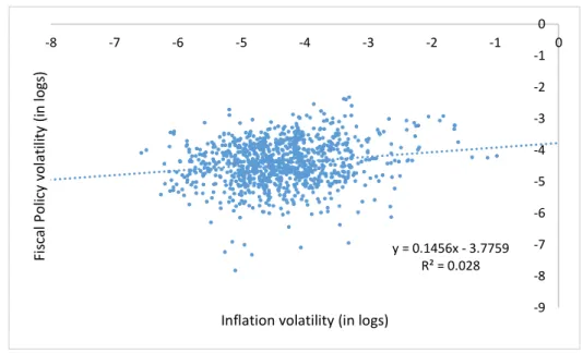
Figure 1 presents a scatterplot of the two key variables in this study, using annual data.

Inflation volatility, measured by the (log of the) 5-year rolling standard deviation of inflation

rates, is presented along the x-axis, while fiscal policy volatility, measured by the (log of)

absolute changes in the cyclically adjusted primary balance, is presented along the y-axis. Even

though the scatter does not show a strong relationship, there appears to be some positive link

between these two variables when other explanatory factors are not accounted for.

Figure 1: Fiscal policy volatility versus inflation volatility (all countries, years)

Note: authors’ calculations.

4.2 Baseline Regression

We now move on into estimating Equation (3). Table 1 shows the results for three variants

of the baseline specification where i) one lag of the dependent variable is included in the set of

regressors, ii) one lag of the dependent variable and one lag of inflation rate are included in the

set of regressors; iii) two lags of the dependent variable and one lag of inflation rate are included

in the set of regressors. Moreover, we present OLS results without time or country fixed effects,

with country fixed effects and with both country and time effects. Looking at the estimated

coefficients, all of them have the expected signs when significant. More specifically, an increase

in the level of inflation, a widening of the output gap (overheating), a higher share of imports in

y = 0.1456x - 3.7759 R² = 0.028

-9 -8 -7 -6 -5 -4 -3 -2 -1 0

-8 -7 -6 -5 -4 -3 -2 -1 0

F

is

ca

l

P

o

li

cy

v

o

la

ti

li

ty

(

in

l

o

g

s)

(11)

GDP bringing in the influence of external prices and higher nominal exchange rate volatility, all

raise price volatility. Larger governments do seem to moderate fluctuations in prices but

corresponding estimates are not statistically different from zero in this table. Also, volatility

monetary policy, while yielding positive coefficient estimates is not statistically significant at

usual levels. More importantly, our measure of fiscal stance (which in this case takes the form of

the absolute value of annual changes in the CAPB) comes out with positive and statistically

significant coefficients, meaning that heightened fiscal activism adversely affects price stability.

[Table 1]

The size of the impact of the volatility of activist fiscal policies on inflation variability can

be important. Focusing on the last 3 columns of Table 1, the estimated coefficient for fiscal

stance is between 0.025 and 0.033. With a cross-country average of standard deviations of

discretionary fiscal policies of 1.94 percentage points of GDP, this suggests that an increase in

the volatility of activist fiscal policies by one standard deviation raises inflation volatility

between 5 and 6 percent. To this direct impact, the indirect impact of the volatility of

discretionary fiscal policies through their impact on output gap variability needs to be added.

Based on a comprehensive survey of the literature, Hemming et al. (2002) report a likely size of

the short-run fiscal multiplier between one half and one. Combining the average of these values

(3/4) with the coefficient on output gap variability yields a potential additional impact between

1.5 and 3.5 percent, resulting in a total impact between 6.5 and 9.5 percent for the average across

the sample. Feedback effects through the interaction of fiscal discretion with the other

explanatory variables would increase the impact further.

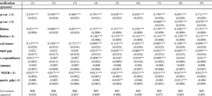
In Table 2 we replace our measure of fiscal stance by the 5-year rolling standard deviation

of the CAPB. Results are generally in line with those reported in Table 1. Now government size

(proxied by public expenditures) yields a negative and statistically significant coefficient,

confirming the theoretical role of automatic stabilizers in attenuating general fluctuations. For the

remainder of the analysis we will use the absolute value of annual changes in the CAPB as our

preferred measure for the fiscal stance and include country and time effects in our estimations.

(12)

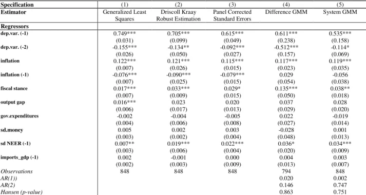
4.3 Robustness to alternative estimators and sensitivity to outliers

It is important to subject our Equation (3) to alternative estimators that help correcting and

overcoming some of the traditionally encountered econometric pitfalls. First, a positive

correlation between inflation volatility and fiscal stance can also be the result of reverse causality,

i.e., higher inflation volatility causing more activist fiscal policies. In addition, the results can be

driven by a third, omitted variable that affects inflation volatility and the volatility of

discretionary fiscal policies simultaneously. If we correctly specify the form of the variance (that

is, if we account for serial correlation and possible cross-sectional heteroskedasticity and then use

estimated cross-section residual variances as weights), then there exists a more efficient estimator

(Feasible Generalized Least Squares, FGLS) than OLS.

Endogeneity between right and left hand side variables can be an additional concern. In an

attempt to overcome this issue we resort to Arellano and Bond (1991) difference GMM estimator

(DIF-GMM). 8_{However, as there are a number of limitations of DIF-GMM estimation}9_{, under the}

assumptions set in Arellano and Bover (1995), the system-GMM estimator (SYS-GMM) can be

used to alleviate the weak instruments problem. The SYS-GMM jointly estimates the equations

in first differences, using as instruments lagged levels of the dependent and independent

variables, and in levels, using as instruments the first differences of the regressors.10_Intuitively,

the system-GMM estimator does not rely exclusively on the first-differenced equations, but

exploits also information contained in the original equations in levels.

We also employ the panel-corrected standard error (PCSE) estimator by Beck and Katz

(1995). Finally, we run of main regression equation with Driscoll-Kraay (1998) robust standard

errors. This non-parametric technique assumes the error structure to be heteroskedastic,

autocorrelated up to some lag and possibly correlated between the groups.

8_{The GMM approach estimates parameters directly from moment conditions imposed by the model. To enable}

identification the number of moment conditions should be at least as large as the number of unknown parameters. Moreover, the mechanics of the GMM approach relates to a standard instrumental variable estimator and also to issues such as instrumental validity and informativeness.

9_{For instance, the lagged levels of the series may be weak instruments for first differences, especially when they are}

highly persistent, or the variance of the individual effects is high relative to the variance of the transient shocks

10_{As far as information on the choice of lagged levels (differences) used as instruments in the differences (levels)}

(13)

Table 3 shows the results. We observe consistent results across the different estimators, from

column (1) to (5). Specifically, higher inflation or nominal exchange rate fluctuations enhances

price volatility. The same is true if fiscal policy becomes more active (in discretionary terms).

The positive impact of the output gap is only statistically significant in the FGLS regression.

[Table 3]

Another important aspect to take into consideration is how much outliers drive our results,

particularly when the sample is heterogeneous and includes emerging market economies that are

usually characterized by spells of hyper-inflations every now and then. We use several alternative

methods to exclude potentially adverse outliers form our estimations. First, we employ the Least

Absolute Deviations (LAD) estimation method which is a robust method in the presence of

outliers and asymmetric error terms (Bassett and Koenker, 1978). Second, we use the M

estimation which was introduced by Huber (1973). Third, the S estimation that is a high

breakdown value method introduced by Rousseeuw and Yohai (1984). Finally, the MM

estimation, introduced by Yohai (1987), combines high breakdown value estimation and M

estimation. It has both the high breakdown property and a higher statistical efficiency than S

estimation.

Looking at Table 4, with the exception of the S estimator, the remaining show a positive

and significant impact of fiscal activism on inflation volatility. The other regressors keep the

previous signs and similar magnitudes.

[Table 4]

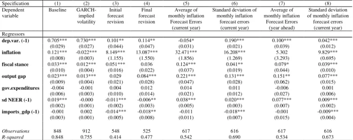
4.4 Using alternative proxies of inflation volatility

In this sub-section we allow for alternative measures of inflation volatility to play a role

as the dependent variable. We consider the set of proxies discussed in Section 3, namely the

GARCH (1,1) implied volatility, the average and standard deviation of 12 months (over the

current year and year-ahead) forecast errors using Consensus Economics forecasts of inflation

and, finally, final and initial forecast revisions of inflation using the same source.

Table 5 includes the baseline for comparison purposes and shows that changes in the

fiscal stance robustly increase price volatility. This means that fluctuations in both actual

inflation data and also in inflation expectations, reflecting different horizons of uncertainty, are

(14)

[Table 5]

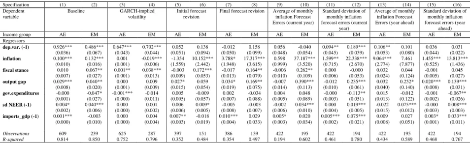
In Table 6 we repeat the same set of estimations as in Table 5 but we split our sample by

income group into advanced and emerging countries. In general, fiscal activism in emerging

market economies fuels inflation volatility much more pronouncedly compared to advanced

countries. High inflation by itself has also a more damaging effect in price fluctuations in

emerging markets than in advanced countries.

[Table 6]

4.5 Fiscal activism, good and bad times and financial crises

We go in exploring whether fiscal activism is different during good and bad times of the

economic business cycle. To this end, we interact our measure of fiscal volatility with positive

and negative output gap. We observe in Table 7 that during economic expansions (recessions) the

detrimental effect of fiscal activism on price volatility is soften (heightened). Going one step

further, and focusing on bad times or recessionary periods, we interact our fiscal stance measure

with dummy variables for financial crises, banking crises and currency crises (retrieved from

Leaven and Valencia, 2008, 2010). Particularly during currency crises, which themselves

increase inflation volatility, discretionary fiscal policy actions tend to exacerbate the price

volatility impact.

[Table 7]

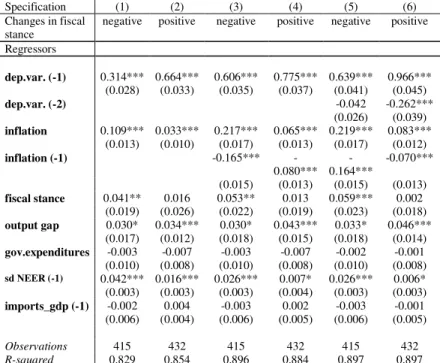
4.6 Fiscal activism and asymmetric effects

Finally, does our measure of fiscal stance defined as the absolute value of annual changes

in the CAPB have differentiated effects is those changes mean an improvement or a deterioration

of the fiscal stance? We explore this by splitting our proxy for fiscal volatility into the absolute

value of positive changes and the absolute value of negative changes. Table 8 shows that the

negative impact of increased fiscal activism in price stability is particularly high during times of

budgetary expansion. When the budgetary position is improving, that is, the CAPB improves

between two years, by means of fiscal consolidation, the effect of discretionary fiscal actions on

price volatility is not statistically different from zero.

(15)

5. Conclusion

The links between fiscal policy and inflation are important in terms of inflationary

pressures from fiscal expansions and also regarding the potential instability effects of government

activities on price volatility.

In his paper, we have used a panel sample of 54 countries covering both advanced and

emerging economies between 1980 and 2013, and we found empirical support for the view that

changes in the fiscal policy stance show a significant positive correlation with inflation volatility.

In addition, after accounting for possible endogeneity between right and left hand side variables,

using the difference GMM estimator, we still found similar results. Therefore, more active fiscal

policy increases price volatility.

Moreover, we have also resorted to alternative measures of inflation volatility: GARCH

(1,1) implied volatility; the average and standard deviation of 12 months forecast errors using

Consensus Economics forecasts; final and initial forecast revisions of inflation using the same

source. Our results using different inflation volatility proxies confirm that expansionary fiscal

stance augments price volatility.

Taking into account the two sub-samples of advanced and emerging economies, fiscal

activism fuels inflation volatility much more pronouncedly in the case of emerging market

economies vis-a-vis advanced economies.

Another relevant result relates to the fact that in a context of economic expansions

(recessions) the harmful impact of fiscal activism on price volatility is soften (heightened). In the

same vein, the negative impact of fiscal activism on price stability is higher when fiscal policy is

expansionary. This has a useful policy implication since hints at the idea that discretionary fiscal

policy can produce less price volatility in boom times. On the other hand, in the context of a

(16)

References

1. Afonso, A. and Gomes, P. (2014). “Interactions between private and public sector wages”, Journal of Macroeconomics, 39, 97-112.

2. Afonso, A., Sousa, R. (2012). “The Macroeconomic Effects of Fiscal Policy”, Applied Economics, 44 (34), 4439-4454.

3. Al-Marhubi, F. (1998), “Cross-country evidence on the link between inflation volatility and growth”, Applied Economics, 30, 1317–1326.

4. Arellano, M. and O. Bover (1995), “Another look at the instrumental variable estimation of error-components models”, Journal of Econometrics, 68, 29–51.

5. Arellano, M. and S. Bond (1991), “Some tests of specification for panel data: Monte Carlo evidence and an application to employment equations”, Review of Economic Studies, 58, 277–297.

6. Artis, M.J. (1996), "How accurate are the IMF's short term forecasts? Another examination of the World Economic Outlook", IMF Research Department Working Paper.

7. Bassetto, M., Butters, R. (2010). “What is the relationship between large deficits andinflation in industrialized countries?”oEconomic Perspectives 3Q/2010, 83-100, Federal Reserve Bank of Chicago

8. Bassett, G., and Koenker, R. (1978), ”Asymptotic Theory of Least Absolute Error Regression”, Journal of the American Statistical Association, 73(363), 618-622.

9. Batchelor, R. and Dua, P. (1995), "Forecaster diversity and the benefits of combining forecasts", Management Science, 41, 1, 68-75.

10. Beck, N. and J. N. Katz (1995), What to do (and not to do) with time-series cross-section data, American Political Science Review 89, 634{47.

11. Blanchard, O. and J. Simon (2001), “The Long and Large Decline in U.S. Output Volatility”, Brookings Papers on Economic Activity, 1,135–164

12. Browsher, C. G. (2002), “On testing overidentifying restrictions in dynamic panel data models”, CEPR Discussion Paper No. 3048, CEPR London.

13. Catão, L., Terrones, M. (2003). “Fiscal Deficits and Inflation”, IMF WP 03/65.

(17)

15. Driscoll, J. and Kraay, A.: (1998), Consistent covariance matrix estimation with spatially dependent panel data, Review of Economics and Statistics 80(4), 549ñ560.

16. Fatas, A., and I. Mihov (2003), “The case for restricting fiscal policy discretion”, Quarterly Journal of Economics, 4, 1419–1447

17. Fischer, S., Sahay, R., Végh, C. (2002). "Modern Hyper- and High Inflations." Journal of Economic Literature, 40 (3), 837-880.

18. Friedman, M. (1977), “Nobel lecture: Inflation and unemployment”, Journal of Political Economy, 85, 451–472

19. Froyen, R. and R. Waud (1987), “An examination of aggregate price uncertainty in four countries and some implications for real output”, International Economic Review, 28(2), 353– 372.

20. Furceri, D. and Jalles, J. T. (2016), “Determinants and Effects of Fiscal Stabilization: New Evidence from Time-Varying Estimates”, forthcoming IMF Working Paper, Washington DC, USA

21. Hemming, Richard, Kell, Michael and Mahfouz, Selma (2002): The Effectiveness of Fiscal Policy in Stimulating Economic Activity – A Review of the Literature. IMF Working Paper 02/208

22. Huber, P.J. (1973), “Robust regression: Asymptotics, conjectures and Monte Carlo,” Annals of Statistics, 1, 799- 821.

23. Jalles, J. T., Karibzhanov, I. and Loungani, P. (2015), “Cross-country Evidence on the Quality of Private Sector Fiscal Forecasts”, Journal of Macroeconomics, Vol. 45, pp. 186-201

24. Judson, R. and A. Orphanides (1999), “Inflation, Volatility and Growth”, International Finance, 2(1), 117–138

25. Laeven, L. and Valencia, F. (2008). Systemic Banking Crises: A New Database. International Monetary Fund, IMF Working Papers, No 08/224.

26. Laeven, L.., and Valencia, F. (2010). Resolution of Banking Crises: The Good, the Bad, and the Ugly. International Monetary Fund, IMF Working Papers, No 10/146.

27. Leeper, E. (1991). “Equilibria Under 'Active' and 'Passive' Monetary and Fiscal Policies,” Journal of Monetary Economics, 27 (1), 129-147.

(18)

29. Loungani, P., H. Stekler and N. Tamirisa, 2013, “Information Rigidity in Growth Forecasts: Some Cross-Country Evidence,” International Journal of Forecasting, 29, 605–21.

30. Martinez-Mongay, C. (2001), “Some (un-)pleasant econometrics about the relationship between fiscal policy and macroeconomic stability. Stability-enhancing reforms of governments”, mimeo, European Commission, Brussels

31. Melitz, J. (1997), “Some Cross-Country Evidence About Debt, Deficits and the Behaviour of Monetary and Fiscal Authorities”, CEPR Discussion Paper 1653.

32. Muscatelli, V. A.; Tirelli, P.; Trecroci, C. (2002), “Monetary and Fiscal Policy Interactions Over the Cycle: Some Empirical Evidence”, CESifo Working Paper 817

33. Perotti, R. (2002). “Estimating the effects of fiscal policy in OECD countries”, ECB WP 168.

34. Rousseeuw, P. J. and V. J. Yohai, (1984), “Robust Regression by Mean of S Estimators, Robust and Nonlinear Time Series Analysis, New York, 256-274

35. Roodman, D. M. (2009), “A note on the theme of too many instruments”, Oxford Bulletin of Economics and Statistics, 71(1), 135-58.

36. Rother, P. (2004). “Fiscal policy and inflation volatility”, ECB WP 317.

37. Sargent, T. and Wallace, N. (1981). “Some unpleasant monetarist arithmetic,” Federal Reserve Bank of Minneapolis Quarterly Review, 1-17, Fall.

38. Sims, C. (1994). “A Simple Model for the Study on the Determination of the Price Level and the Interaction of Monetary and Fiscal Policy,” Economic Theory, 4 (3), 381-399.

39. Tulip, P. (2014). “Fiscal Policy and the Inflation Target”, International Journal of Central Banking, June, 63-96.

40. Yohai, V. (1987). “High Breakdown Point and High Efficiency Robust Estimates for Regression”, The Annals of Statistics, 15 (20), 642-656.

41. van Aarle, Bas; Garretsen, Harry, and Niko Gobbin (2003), “Monetary and Fiscal Policy Transmission in the Euro area: Evidence from a Structural VAR Analysis”, Journal of Economics and Business, 55 (5-6), 609-638. .

42. Woodford, M. (1994). “Monetary Policy and Price Level Determinacy in a Cash-in-Advance Economy,” Economic Theory, 4 (3), 345-380.

(19)

Table 1: Price Volatility and Fiscal Discretion (measured as the absolute value of fiscal stance)

Specification (1) (2) (3) (4) (5) (6) (7) (8) (9)

Effects No Country Time+country No Country Time+country No Country Time+country

Regressors

dep.var. (-1) 0.528*** 0.425*** 0.429*** 0.687*** 0.588*** 0.613*** 0.797*** 0.686*** 0.700***

(0.022) (0.023) (0.023) (0.022) (0.027) (0.027) (0.029) (0.031) (0.032)

dep.var. (-2) -0.135*** -0.133*** -0.117***

(0.023) (0.023) (0.023)

inflation 0.055*** 0.076*** 0.074*** 0.146*** 0.129*** 0.122*** 0.150*** 0.135*** 0.129***

(0.008) (0.009) (0.010) (0.009) (0.010) (0.010) (0.009) (0.009) (0.010)

inflation (-1) -0.129*** -0.100*** -0.114*** -0.121*** -0.093*** -0.108***

(0.009) (0.010) (0.011) (0.009) (0.010) (0.010)

fiscal stance 0.016 0.031** 0.027** 0.027** 0.035*** 0.032** 0.038*** 0.043*** 0.039***

(0.015) (0.013) (0.014) (0.013) (0.012) (0.013) (0.013) (0.012) (0.013)

output gap 0.029* 0.031** 0.025 0.054*** 0.046*** 0.052*** 0.053*** 0.047*** 0.056***

(0.015) (0.014) (0.016) (0.013) (0.013) (0.015) (0.013) (0.013) (0.015)

gov.expenditures -0.005** -0.009 -0.011 -0.003 -0.012* -0.018** -0.004** -0.009 -0.015**

(0.002) (0.007) (0.008) (0.002) (0.007) (0.007) (0.002) (0.007) (0.007)

sd.money 0.001 0.006 0.003 0.003 0.002 0.005 0.004 0.002 0.005

(0.005) (0.006) (0.006) (0.005) (0.005) (0.006) (0.004) (0.005) (0.005)

sd NEER (-1) 0.023*** 0.030*** 0.030*** 0.013*** 0.019*** 0.017*** 0.012*** 0.019*** 0.017***

(0.002) (0.002) (0.002) (0.002) (0.002) (0.003) (0.002) (0.002) (0.002)

imports_gdp (-1) 0.004*** 0.000 -0.003 0.002** -0.006 -0.004 0.002* -0.007* -0.005

(0.001) (0.004) (0.005) (0.001) (0.004) (0.005) (0.001) (0.004) (0.005)

Observations 723 723 723 723 723 723 723 723 723

R-squared 0.782 0.835 0.848 0.833 0.857 0.872 0.841 0.864 0.877

Note: OLS regression with different sets of time and country effects as identified in the second row. Robust standard errors in parenthesis. *, **, *** denote statistical significance at the 10, 5, and 1 percent levels, respectively. Constant term was estimated by omitted for reasons of parsimony.

Table 2: Price Volatility and Fiscal Discretion (measured as 5-year rolling standard deviation of fiscal stance)

Specification (1) (2) (3) (4) (5) (6) (7) (8) (9)

Regressors

dep.var. (-1) 0.535*** 0.448*** 0.460*** 0.701*** 0.638*** 0.656*** 0.749*** 0.691*** 0.711*** (0.022) (0.024) (0.025) (0.021) (0.025) (0.025) (0.026) (0.028) (0.028)

dep.var. (-2) -0.060*** -0.076*** -0.079***

(0.019) (0.019) (0.019)

inflation 0.071*** 0.098*** 0.097*** 0.157*** 0.157*** 0.150*** 0.159*** 0.160*** 0.153*** (0.009) (0.010) (0.010) (0.009) (0.009) (0.009) (0.009) (0.009) (0.009)

inflation (-1) -0.146*** -0.135*** -0.143*** -0.141*** -0.129*** -0.137***

(0.008) (0.009) (0.009) (0.008) (0.009) (0.009)

fiscal stance 0.137*** 0.190*** 0.172*** 0.089*** 0.116*** 0.103*** 0.085*** 0.109*** 0.099*** (0.029) (0.033) (0.034) (0.025) (0.029) (0.030) (0.025) (0.029) (0.029)

output gap 0.022 0.022 0.030 0.053*** 0.044*** 0.060*** 0.052*** 0.044*** 0.059*** (0.017) (0.017) (0.019) (0.015) (0.015) (0.016) (0.015) (0.015) (0.016)

gov.expenditures -0.011*** -0.007 -0.007 -0.008*** -0.018* -0.019** -0.009*** -0.016* -0.017* (0.003) (0.011) (0.011) (0.002) (0.009) (0.010) (0.002) (0.009) (0.009)

sd.money -0.003 -0.003 -0.007 -0.008 -0.006 -0.001 -0.008 -0.005 0.000 (0.007) (0.008) (0.008) (0.006) (0.007) (0.007) (0.006) (0.007) (0.007)

sd NEER (-1) 0.015*** 0.017*** 0.017*** 0.011*** 0.013*** 0.012*** 0.011*** 0.013*** 0.012*** (0.002) (0.002) (0.002) (0.001) (0.001) (0.002) (0.001) (0.001) (0.002)

imports_gdp (-1) 0.000 -0.003 -0.004 -0.001 -0.010** -0.004 -0.001 -0.011*** -0.004 (0.001) (0.005) (0.006) (0.001) (0.004) (0.005) (0.001) (0.004) (0.005)

Observations 806 806 806 805 805 805 805 805 805 R-squared 0.816 0.842 0.853 0.869 0.880 0.890 0.871 0.883 0.892

(20)

Table 3: Price Volatility and Fiscal Discretion (measured as the absolute value of fiscal stance), alternative estimators

Specification (1) (2) (3) (4) (5)

Estimator Generalized Least Squares

Driscoll Kraay Robust Estimation

Panel Corrected Standard Errors

Difference GMM System GMM

Regressors

dep.var. (-1) 0.749*** 0.705*** 0.615*** 0.611*** 0.535***

(0.031) (0.099) (0.049) (0.238) (0.158)

dep.var. (-2) -0.155*** -0.134** -0.092*** -0.512*** -0.114*

(0.026) (0.050) (0.027) (0.157) (0.069)

inflation 0.122*** 0.121*** 0.115*** 0.117*** 0.119***

(0.007) (0.026) (0.015) (0.023) (0.035)

inflation (-1) -0.076*** -0.090*** -0.079*** 0.029 -0.056

(0.007) (0.025) (0.015) (0.054) (0.038)

fiscal stance 0.017*** 0.033*** 0.029* 0.135*** 0.038**

(0.007) (0.009) (0.015) (0.050) (0.018)

output gap 0.016*** 0.023 0.020 0.037 0.028

(0.006) (0.017) (0.013) (0.029) (0.020)

gov.expenditures -0.002 -0.004 -0.005 0.022 -0.019

(0.004) (0.006) (0.008) (0.027) (0.014)

sd.money 0.005 0.002 0.003 -0.028 0.001

(0.003) (0.002) (0.004) (0.048) (0.013)

sd NEER (-1) 0.007** 0.019*** 0.022*** 0.036* 0.034***

(0.003) (0.006) (0.004) (0.020) (0.009)

imports_gdp (-1) 0.002 -0.001 0.000 0.004 0.003

(0.002) (0.003) (0.009) (0.013) (0.007)

Observations 848 848 848 794 848

AR(1)) 0.020 0.002

AR(2) 0.146 0.747

Hansen (p-value) 0.863 0.751

Note: Estimation using alternative estimators as identified in the second row. Robust standard errors in parenthesis. AR(1) and AR(2) denote the values for the first and second order serial correlation in the residuals. The Hansen p-value tests the null hypothesis of correct model specification and valid overidentifying restrictions, that is validity of the instruments. *, **, *** denote statistical significance at the 10, 5, and 1 percent levels, respectively. Constant term was estimated by omitted for reasons of parsimony.

Table 4: Price Volatility and Fiscal Discretion (measured as the absolute value of fiscal stance), outlier robust

Specification (1) (2) (3) (4)

Estimator LAD M S MM

Regressors

dep.var. (-1) 0.495*** 0.761*** 0.947*** 0.883***

(0.018) (0.036) (0.024) (0.025)

inflation 0.052*** 0.030*** 0.018*** 0.025***

(0.007) (0.007) (0.006) (0.005)

fiscal stance 0.017* 0.015** 0.002 0.014**

(0.010) (0.007) (0.006) (0.006)

output gap 0.021** 0.035*** 0.010* 0.020***

(0.009) (0.008) (0.005) (0.007)

gov.expenditures -0.002 -0.002 -0.001* -0.002

(0.002) (0.001) (0.001) (0.001)

sd NEER (-1) 0.021*** 0.009*** -0.004** 0.002

(0.002) (0.003) (0.002) (0.002)

imports_gdp (-1) 0.004*** 0.002*** -0.000 0.001*

(0.001) (0.000) (0.000) (0.000)

Observations 839 848 848 848

R-squared 0.764

(21)

Table 5: Price Volatility and Fiscal Discretion (measured as the absolute value of fiscal stance), alternative dependent variables

Specification (1) (2) (3) (4) (5) (6) (7) (8)

Dependent variable

Baseline GARCH-implied volatility

Initial forecast revision

Final forecast revision

Average of monthly inflation

Forecast Errors (current year)

Standard deviation of monthly inflation

forecast errors (current year)

Average of monthly inflation

Forecast Errors (year ahead)

Standard deviation of monthly inflation

forecast errors (current year) Regressors

dep.var. (-1) 0.705*** 0.730*** 0.101** 0.114** -0.054* 0.190*** 0.100*** 0.042***

(0.029) (0.027) (0.044) (0.047) (0.031) (0.021) (0.039) (0.012)

inflation 0.121*** -0.022*** 8.149*** 13.087*** 32.471*** 16.208*** 5.302 9.829***

(0.008) (0.003) (1.155) (1.550) (1.856) (1.269) (3.293) (0.695)

fiscal stance 0.033*** 0.012*** 0.051*** 0.036 0.124*** 0.041** 0.079* 0.039***

(0.010) (0.004) (0.016) (0.022) (0.037) (0.019) (0.044) (0.010)

output gap 0.023*** 0.013*** 0.029 0.084*** 0.221*** 0.131*** 0.151** 0.077***

(0.009) (0.004) (0.021) (0.028) (0.047) (0.028) (0.062) (0.015)

gov.expenditures -0.004 -0.001 0.004 0.012 0.014 0.011 -0.006 0.001

(0.006) (0.003) (0.010) (0.014) (0.021) (0.012) (0.027) (0.006)

sd NEER (-1) 0.019*** -0.000 -0.011*** -0.006** 0.038*** 0.020*** 0.077*** 0.009***

(0.002) (0.001) (0.002) (0.003) (0.005) (0.003) (0.007) (0.002)

imports_gdp (-1) -0.001 0.002 -0.014*** -0.018** -0.011 -0.018*** -0.001 -0.009***

(0.003) (0.001) (0.005) (0.008) (0.011) (0.007) (0.015) (0.004)

Observations 848 912 548 525 617 616 617 616 R-squared 0.848 0.755 0.414 0.477 0.542 0.690 0.534 0.673

(22)

Table 6: Price Volatility and Fiscal Discretion (measured as the absolute value of fiscal stance), alternative dependent variables, by income group

Specification (1) (2) (3) (4) (5) (6) (7) (8) (9) (10) (11) (12) (13) (14) (15) (16)

Dependent variable

Baseline GARCH-implied volatility

Initial forecast revision

Final forecast revision Average of monthly inflation Forecast Errors (current year)

Standard deviation of monthly inflation forecast errors (current

year)

Average of monthly inflation Forecast Errors (year ahead)

Standard deviation of monthly inflation forecast errors (year

ahead)

Income group AE EM AE EM AE EM AE EM AE EM AE EM AE EM AE EM

Regressors

dep.var. (-1) 0.926*** 0.486*** 0.647*** 0.702*** 0.052 0.138 -0.012 0.158 0.056 -0.040 0.094** 0.189*** 0.106** 0.101 0.036 0.031 (0.036) (0.067) (0.043) (0.044) (0.051) (0.094) (0.050) (0.099) (0.048) (0.054) (0.045) (0.039) (0.053) (0.080) (0.044) (0.022)

inflation 0.100*** 0.132*** 0.001 -0.019*** -1.354 10.152*** 3.788* 17.317*** 0.598 37.187*** 1.599** 22.338*** 9.064*** 7.461 1.455*** 13.813*** (0.010) (0.016) (0.001) (0.006) (1.559) (2.442) (1.948) (3.615) (0.999) (3.520) (0.715) (2.670) (2.774) (7.877) (0.525) (1.436)

fiscal stance 0.010 0.067** 0.001** 0.038*** -0.003 0.172*** -0.017 0.164** -0.006 0.262** 0.000 -0.000 0.032 0.044 -0.001 0.045 (0.007) (0.027) (0.001) (0.013) (0.009) (0.053) (0.013) (0.079) (0.010) (0.109) (0.006) (0.053) (0.024) (0.124) (0.005) (0.027)

output gap 0.029*** 0.040** 0.000 0.009 0.027* 0.059 0.034* 0.169** -0.007 0.390*** -0.012 0.235*** 0.032 0.252* 0.020*** 0.139*** (0.008) (0.020) (0.001) (0.009) (0.015) (0.054) (0.019) (0.075) (0.014) (0.113) (0.010) (0.061) (0.040) (0.140) (0.008) (0.031)

gov.expenditures -0.000 -0.047* -0.001*** -0.014 0.005 -0.009 0.002 -0.034 0.004 0.048 -0.000 -0.113** 0.015 -0.012 -0.001 -0.067** (0.001) (0.027) (0.000) (0.011) (0.005) (0.057) (0.007) (0.088) (0.005) (0.089) (0.003) (0.051) (0.013) (0.122) (0.002) (0.026)

sd NEER (-1) 0.004* 0.040*** 0.000 0.001 0.006 0.009* -0.005 -0.003 -0.002 0.034*** 0.000 0.019*** -0.022 0.075*** -0.000 0.008*** (0.002) (0.006) (0.000) (0.002) (0.006) (0.005) (0.008) (0.007) (0.006) (0.010) (0.004) (0.005) (0.015) (0.012) (0.003) (0.003)

imports_gdp (-1) 0.001*** -0.003 0.000 0.004 0.007** -0.018 0.010*** 0.029 0.005* 0.020 0.005*** 0.075*** 0.009 0.027 0.003* 0.033*** (0.000) (0.010) (0.000) (0.004) (0.003) (0.019) (0.004) (0.033) (0.003) (0.034) (0.002) (0.021) (0.008) (0.051) (0.001) (0.011)

Observations 609 239 625 287 397 151 386 139 422 195 422 194 422 195 422 194 R-squared 0.814 0.850 0.752 0.796 0.352 0.484 0.354 0.497 0.194 0.602 0.461 0.780 0.434 0.589 0.468 0.767

(23)

Table 7: Price Volatility and Fiscal Discretion (measured as the absolute value of fiscal stance), recessions and financial crises

Specification (1) (2) (3) (4)

Regressors

dep.var. (-1) 0.538*** 0.394*** 0.532*** 0.526***

(0.020) (0.035) (0.020) (0.020)

inflation 0.052*** 0.089*** 0.053*** 0.057***

(0.007) (0.015) (0.007) (0.007)

fiscal stance 0.023** 0.039 0.022** 0.021*

(0.010) (0.024) (0.011) (0.011)

output gap 0.023** 0.028* 0.028*** 0.021**

(0.009) (0.017) (0.010) (0.010)

gov.expenditures -0.003 0.005 -0.003 -0.003

(0.002) (0.005) (0.002) (0.002)

sd NEER (-1) 0.023*** 0.041*** 0.023*** 0.025***

(0.002) (0.005) (0.002) (0.002)

imports_gdp (-1) 0.004*** 0.004*** 0.004*** 0.004***

(0.001) (0.001) (0.001) (0.001)

Recession* fiscal stance 0.100*** (0.032)

Expansion* fiscal stance -0.083** (0.040)

FC 0.004

(0.003)

FC* fiscal stance 0.181

(0.173)

banking 0.002

(0.001)

Banking* fiscal stance 0.158* (0.082)

currency 0.006**

(0.003)

Currency* fiscal stance 0.196* (0.102)

Observations 848 282 848 848

R-squared 0.775 0.747 0.775 0.775

(24)

Table 8: Price Volatility and Fiscal Discretion, asymmetric effects to fiscal expansions and consolidations

Specification (1) (2) (3) (4) (5) (6)

Changes in fiscal stance

negative positive negative positive negative positive

Regressors

dep.var. (-1) 0.314*** 0.664*** 0.606*** 0.775*** 0.639*** 0.966*** (0.028) (0.033) (0.035) (0.037) (0.041) (0.045)

dep.var. (-2) -0.042 -0.262*** (0.026) (0.039)

inflation 0.109*** 0.033*** 0.217*** 0.065*** 0.219*** 0.083*** (0.013) (0.010) (0.017) (0.013) (0.017) (0.012)

inflation (-1) -0.165*** -0.080***

-0.164***

-0.070***

(0.015) (0.013) (0.015) (0.013)

fiscal stance 0.041** 0.016 0.053** 0.013 0.059*** 0.002 (0.019) (0.026) (0.022) (0.019) (0.023) (0.018)

output gap 0.030* 0.034*** 0.030* 0.043*** 0.033* 0.046*** (0.017) (0.012) (0.018) (0.015) (0.018) (0.014)

gov.expenditures -0.003 -0.007 -0.003 -0.007 -0.002 -0.001 (0.010) (0.008) (0.010) (0.008) (0.010) (0.008)

sd NEER (-1) 0.042*** 0.016*** 0.026*** 0.007* 0.026*** 0.006* (0.003) (0.003) (0.003) (0.004) (0.003) (0.003)

imports_gdp (-1) -0.002 0.004 -0.003 0.002 -0.003 -0.001 (0.006) (0.004) (0.006) (0.005) (0.006) (0.005)

Observations 415 432 415 432 415 432

R-squared 0.829 0.854 0.896 0.884 0.897 0.897

(25)

APPENDIX List of countries

United States, United Kingdom, Austria, Belgium, Denmark, France, Germany, Italy, Netherlands, Norway, Sweden, Switzerland, Canada, Japan, Finland, Greece, Iceland, Ireland, Portugal, Spain, Turkey, Australia, New Zealand, South Africa, Argentina, Brazil, Chile, Colombia, Mexico, Peru, ,Israel ,Jordan , Egypt, Hong Kong SAR, India, Indonesia, Korea, Malaysia, Philippines, Singapore, Thailand, Morocco, Bulgaria, Russia, China, Ukraine, Czech Republic, Slovak Republic, Hungary, Lithuania, Slovenia, Poland, Romania.

Table A1: Correlation between measures of inflation volatility

Correlation coefficients 5-year rolling standard

deviation of inflation

GARCH(1,1) implied volatility 0.0906***

12 average of inflation forecast errors (current year) 0.1633***

12 standard deviation of inflation forecast errors (current year) 0.582***

12 average of inflation forecast errors (year ahead) 0.3146***

12 standard deviation of inflation forecast errors (year ahead) 0.5206***

Final forecast revision 0.2812***

Initial forecast revision 0.2352***

Note: *** denote statistical significant at the 1 percent level.

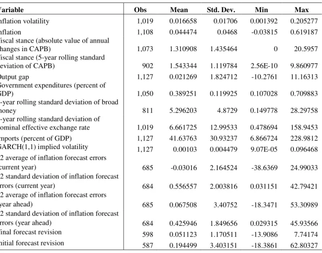
Table A2: Summary Statistics