1
The economic role of housework at retirement and personality traits:
evidence from the United Kingdom
Bernardo Fonseca Nunes, University of Stirling
This draft: 10
thJuly 2014
Abstract
Housework is a crucial determinant of expenditure patterns at retirement by acting as a substitute for the purchase of market goods and services. In this paper we build on the literature about retirement behaviour by revisiting the economic role of home-production of good and services. Specifically, we empirically examine whether personality traits determine the time individuals devote to housework due to the occurrence of a transition to retirement. Our empirical strategy is organized by studying the constraints of a two-period model of transition to retirement which has housework as a component of agents’ life-time wealth. Then, we use longitudinal data from the British Household Panel Survey – of individuals aged 55 or above to show that extraversion is a key determinant of the changes in the time new retirees devote to these tasks, being more relevant than consumption expenditures, household income, and gender. Extroverted individuals are not only oriented by productivity but might also perceive activities such as cooking for household members and doing grocery shopping, as less costly in terms of effort, or even pleasant. More extroverted retirees might also do housework to sustain their pre-retirement levels of leisure and entertainment expenditures. We provide findings that could be useful for policymakers in the field of pensions and social care to better understand how the ageing population cope with expenditures and adapt its economic behaviour to achieve desired standards of living at retirement.
JEL classification: D13, E21. 1. Introduction
Housework acquires a crucial economic role on the explanation of expenditure patterns at retirement when household members devote time to home-production of meals, cleaning and laundry. Despite being a substitute for the purchase of market goods and services (Luengo-Prado and Sevilla, 2013), housework is not included as a component of an individual’s inter-temporal constraints in economic descriptive models of transition to retirement. Alongside financial determinants, the decision to do housework depends not only on the physical and mental abilities needed to perform related tasks. It might also be determined by an individual’s comparative advantages in the form of non-cognitive skills, as suggested by literature on the integration of personality measures in economic models (Heckman, Stixrud and Urzuo, 2006; Almlund et al., 2011). The Big Five personality traits (Costa and McCrae, 1992) - openness to experience, conscientiousness, extraversion, agreeableness and neuroticism – have been established as predictors of early and later life outcomes (Heckman, 2011). In this paper we build on the literature about retirement behaviour
2
by revisiting the economic role of home-production of good and services. Specifically, we empirically examine whether personality traits determine the time individuals devote to housework due to the occurrence of a transition to retirement.
At retirement, a set of economic decisions need to be done. Labour income ceases to be a relevant part of individuals’ endowments and money inflows become exogenous, given previous private savings or a state-provided pension. Work-related consumption, e.g. meals near the job place, transportation, clothing and training, loses relevance. Retirees are able to allocate part of their new endowment of time to domestic activities, such as. Time is usually redirected from paid labour to tasks which demand different levels of effort and ability, e.g. physical activity, leisure, and housework. Individuals might also increase housework to economize monetary income and pay for desired expenditures when direct substitution is not possible, as in the case of paid leisure activities, entertainment and travelling.
Empirical studies have shown that consumption expenditure shows a discrete drop at retirement, leading to a conventional view that the only way to reconcile the fall in consumption around the time of retirement with the implication of forward-looking models was given by the arrival of unexpected adverse information. This phenomenon, which became known in the early literature as the “retirement savings puzzle”, was documented in the United Kingdom (Banks et al, 1998) and in other major countries: the United States (Hamermesh, 1984; Mariger, 1987; Bernheim et al., 2001; Haider and Stephens, 2007), Canada (Robb and Burbidge, 1989), Italy (Battistin et al., 2009; Miniaci et al., 2010) and Germany (Schwerdt, 2005). Alternatively, Luengo-Prado and Sevilla (2013) analysed household expenditures from a broad selection of goods and services in Spain. They suggest that a fall in expenditure on food and groceries upon retirement does not necessarily correspond to reduced food consumption due to the fact that retirees receive an additional endowment of time and become able to perform domestic activities, such as cooking at home and grocery shopping, replacing some market goods with home-produced goods. Despite their rich insights about the economic role of housework at retirement, the authors present only cross-sectional estimates of the retirement effect on the time devoted to shopping, cooking and eating activities.
There are few analyses of the relationship between personality traits and retirement (Robinsonet al, 2010; Spetch et al. 2011, Blekesaune and Skirbekk, 2012) but none have empirically approached whether personality determines economic behaviour at the moment of retirement. Additionally, gender has become a key source of heterogeneity in the life course transition from the labour market to retirement since it is not
3
passage associated principally to male individuals (Moen et al., 2001). Women experience housework differently as a consequence of their career and marital status (Bryan and Sevilla-Sanz, 2011) and of gendered expectations that poses a barrier to the equality of domestic division of labour (Kan, 2012), facts that might be also influenced by personality traits at retirement.
Our empirical strategy is organized by studying the constraints of a two-period model of transition to retirement which has housework as a component of agents’ life-time wealth. Then, we use longitudinal data from the British Household Panel Survey – BHPS1, waves 15 to 18 (2005-2008) of individuals aged 55 or above to implement a potential outcomes framework (Cameron and Trivedi, 2005, p. 862) in which the change in an individual weekly housework hours is the dependent variable, and the occurrence of a transition to retirement from the labour market is the treatment variable. In order to build a counterfactual, we compare the observed housework changes at retirement with respect to a control group composed by observations of individuals who stayed in the labour market for an additional year. Standardized scores of the Big Five personality traits are included as covariates and interacted with the treatment variable. Household and individual consumption expenditures expected to be associated with housework, such as eating out, grocery and leisure expenditures are included in levels and first differences. Socio-demographic and labour market characteristics are included as control variables.
The panel characteristic of the BHPS allows us to extend the empirically limited cross-sectional analysis of Luengo-Prado and Sevilla (2013) of retirees’ time use. First, the BHPS’s fifteenth wave (2005) includes a 15-item questionnaire aiming to measure the respondents’ personality profiles according to the Big Five factors. We use the corresponding individual standardized scores as covariates in our analysis, and test the significance of their interactions with the treatment variable indicating a transition to retirement. Personality might change over the life-cycle or given life circumstances (Costa and McCrae, 2006). For this reason, our sample comprises only transitions to retirement that occurred in waves after corresponding individual traits were measured within a 4-year horizon. Second, we can exploit the empirical advantages of a potential outcomes framework to the estimation of causality in observational (nonrandomized) studies. We observe outcomes for the two groups in two subsequent periods following a difference-in-difference setting
1 The BHPS was launched in 1991 as the UK’s first socio-economic household panel survey with ten thousand people living in 5,500 households in 250 areas of Great Britain selected to become participants. The BHPS has eighteen waves of data that were collected by surveying people annually until 2008, when it was incorporated into another national longitudinal study, Understanding Society.
4
(Cameron and Trivedi, 2005, p. 878; Imbens and Wooldridge, 2007). One group enters retirement in the second period, but is in the labour market in the first period. The counterfactual group does not experience retirement during either period. This helps to mitigates biases form comparison over time in observation of individuals who entered retirement that could be the result of trends, as well as biases in follow-up period comparisons between those who entered retirement and those in the control group that could be the result from permanent group differences.
Our findings show that the average retirement effect on housework is positive, for both men and women, and identify extraversion as the key determinant of the changes in the time new retirees devote to these tasks, being more relevant than consumption expenditures, household income, and gender. Among the adjectives of extroverted people are pro-activity, being energetic, and orientated towards people. They might not be only oriented by productivity and perceive housework activities, such as cooking for household members and doing grocery shopping, as less costly in terms of effort, or even pleasant. Housework also might allow more extroverted retirees to sustain their pre-retirement levels of leisure and entertainment habits by acting as a substitute for other services that they otherwise would have to pay. The observed changes in housework co-vary with household grocery and food bills and housing costs, as well with individual leisure expenditures. These findings contribute to the literature about older people’s consumption patterns, which reports the existence of a cluster of households with constrained incomes that present a particularly high expenditure on food and non-alcoholic drinks. Such households might have a preference for dining at home, entertaining others, or have age-related dietary needs supplied at home (Hayes and Finney, 2014, p. 110).
Finally, our analysis provides conclusions that could be useful for policymakers in the field of pensions and social care to better understand how the ageing population cope with finances and adapt its economic behaviour to achieve desired standards of living. Housework is shown to be a key component of agents’ life-cycle wealth, and mainly determined by non-cognitive skills in the form of personality traits.
This paper is organized as follows. Section 2 presents the conceptual framework of the two-period economic model of transition to retirement which structures our empirical strategy. Section 3 details the method and sampling procedure. Section 4 discusses the main results and robustness checks. Section 5 concludes.
5
2. Conceptual framework
This section presents a stylized two-period economic behaviour model of a transition to retirement. We start by following the individual saving for retirement problem presented in traditional economic models such as the overlapping generations’ model (Samuelson, 1958; Diamond, 1965). We setup the agent’s choice problem and include housework as a component of individual life-time wealth by adopting a similar framework to the one used by Chetty et al (2012). The authors characterized the comparative statics of a two-period model to structure their empirical analysis of saving behaviour given the introduction of government policies such as price subsidies or automatic contribution to pension schemes. In our setup, housework appears as a component of the agent’s inter-temporal constraints and is an additional source of funding for consumption. Later, we motivate the inclusion of personality traits as covariates in our empirical analysis according to the comparative advantage theories presented by Heckman, Stixrud and Urzuo (2006), Almlund et al. (2011) and Heckman (2011).
2.1 Setup
Time is discrete and individuals live for two periods. In the first period, they participate in the labour market and earn a fixed amount , which they can either consume or save in a private savings account aiming to afford consumption later in life. Considering that the postponed consumption in the form of private savings is capitalized by a risk-free rate, and goods and services bought in the first period cannot be stored, real consumption in each period can be described by:
(2.1)
(2.2)
Individuals have utility given by:
(2.3)
where the period utility function is increasing in consumption, reflecting the fundamental desire for more consumption2; and denotes the individual subjective discount factor. Individuals choose according to
2 In the case of a concave it would also reflect aversion to risk and to inter-temporal substitution, or the consumer’s preference for a consumption path that is steady over time and across states of nature.
6
their period utility , satisfying the inter-temporal budget constrain given by the combination of (1) and (2):
(2.4)
The equality described above can be interpreted as the life-time wealth of the individual. Individuals also might engage in home production of goods and services which they would have to buy in the market otherwise, such as cooking, cleaning, and doing laundry. Housework levels are set given the comparative advantages individuals face in each period between paying for housework related items and producing them by themselves.
In order to accommodate these additional features in the model, we propose that consumption in each period to be described:
(2.1’)
(2.2’)
where and are potential new features induced by public policy3 or individual active choice. In the case when housework is a determinant of consumption in each period that cannot be stocked from period 1 to period 2, but might affect the decision of the working-age individuals, we have that and
.
The inter-temporal budget constraint or life-time wealth can now be described by:
(2.4’)
Note that the last term in the right hand side can be interpreted as the present value of a pension or the present value of home production of goods and services during retirement. We assume there are no governmental pension policies, but private savings. Individuals are able to postpone consumption by saving in the first period and to produce goods and services at home in both periods.
3 For example, in the case of a fully funded mandatory pension, and
, which means that the
government collects taxes T from the working-age population and returns them with interest in the next period as a transfer. In a pay-as-you-go system, the transfers to the retired are covered by the tax collection T in the same period, so
and , where is the population growth rate. In Chetty et al’s (2012) model,
and , where is an automatic mandated contribution to a pension account; denotes
voluntary contributions to a retirement account; and is the extra-return generated by a price subsidy given as an incentive when saving for retirement by using and .
7
In this sense, consumption in each period is described by:
(2.1’’)
(2.2’’)
And life-time wealth given by:
Now consider that and , so we can also combine (2.1’’) and (2.2’’) to get:
(2.5) where is a proxy for the available income in t+1; is the part of real consumption in t from the purchase of market goods and services with money income. If an individual desires to smooth consumption during his transition to retirement, not only savings, but also home production of part of his consumption in t+1 is a possibility, and this desire would be reflected in the utility function in (2.3). In the same way, when the replacement rate of income during retirement is close to the unity, i.e., almost no drop in income, the individual is able to make use of his, now available, time endowment and substitute the purchase of market goods and services by home production.
By isolating we can observe that housework is expected to co-vary with real consumption changes, with available money income and with expenditures over market goods and services with money income in the first period.
(2.6)
In sum, by analysing the underlying inter-temporal constraints of this two-period model of transition to retirement, we find theoretical support for the empirical study of the relationship between a transition to retirement and housework production.
2.2 Including personality traits
Next, we discuss the theoretical motivation for including personality traits as covariates in our empirical tests. Non-cognitive skills in the form of personality traits, such as openness to experience,
8
conscientiousness, extraversion, agreeableness, and neuroticism, are potential determinants of a change in housework when the individual retires.
First, we take equation (2.2’’) which represents consumption at retirement and drop its time subscripts, assuming real monetary income as given by .
(2.7)
where C is real consumption of final goods and services; is the exogenous flow of monetary income; and is home production of good and services to own consumption, or simply housework.
In this sense, housework h can be described as a task which outcome depends on productivity , which itself is a function of individual actions taken , traits and effort .
( ) { } (2.8)
We assume personality traits are individual endowments, and that choices are determined by traits and effort, as they affect productivity in tasks (Heckman, 2011). Effort is also an endowment and when it increases in one task it might diminish in another, leading to the restriction ∑ ̅. Productivity is assumed to be increasing in effort. Effort can complement traits,
, or be a substitute to them,
In order to generalize the notion of effort to a broader class of behaviours, let’s assume that actions themselves also depend on traits , effort , and situation , and let be the set of actions, including those ones not directly contributing to productivity.
(2.9)
Agents may not only have preferences over consumption of final goods and services, but also may value the output of the task, the effort and actions devoted to it in their own right. In this sense, the agent solves
s.t (2.7) (2.10)
According to this setup, a transition to retirement is a situation s, which might affect housework given (2.6) and (2.7). Home production might co-vary with changes in the consumption basket, because it acts as a substitute for market goods and services like meals, cleaning and laundry. When there is no possible
9
substitution, like in the case of some paid leisure activities (entertaining and travelling, for example), adjustments in housework levels allow them to economize the exogenous flow of income to pay for these expenditures. The inclusion of personality traits – or non-cognitive skills - as covariates here is due to their association with the actions taken in response to new constraints, endowments and incentives facing agents given their preferences (Heckman, 2011, p. 20). Additionally to the effect of traits through consumption reallocation given a transition to retirement, there might be direct effects due to individuals having preferences over the actions taken during the task itself, including those ones not directly contributing to productivity, such as cooking or grocery shopping, in our particular example.
3. Empirical strategy
We use data from the British Household Panel Survey – BHPS of individuals aged 55 or above during the waves 15 to 18 (2005-2008). Since its second wave, this survey has information on the amount of hours individuals spend on housework on average per week, such as time spent cooking, cleaning and doing the laundry. Figure 1 plots weekly average hours of housework of employed and retired individuals by gender. Women do more housework in both job market statuses. Both genders have higher levels of housework at the retired status compared with an employed status. The observed decrease in housework hours done by women in both status (employed and retired) and by retired men, does not seem to be accompanied by a similar pattern for employed males. In sum, there are not only housework gaps between genders, but also within gender in terms of employed individuals compared with retirees.
Particularly the BHPS’s wave surveyed in 2005 responded fifteen questions capturing the respondent’s personality profile according to the Big Five factors model: openness to experience, conscientiousness, extraversion, agreeableness, and neuroticism. Each of the five personality traits score is measured by a set of three questions, with answers ranging in a scale from 1 – “does not apply” to 7 – applies perfectly”. Then, in order to assess the internal consistency within each set of three questions capturing the five personality traits, we estimate the standardized alpha reliability indexes under the assumptions of the measurement error model of Cronbach (1951). The corresponding alpha indexes are equal to 0.6725, 0.5112, 0.5375, 0.5277, and 0.6750 for openness, conscientiousness, extraversion, agreeableness, and neuroticism respectively. They are very similar to the reliability indexes obtained by Heineck (2007) and Nandi and Nicoletti (2009) who also uses the BHPS, and also similar to the ones obtained by Heineck and Anger (2010)
10
who use the German Household Panel survey with the same personality inventory composed by five traits and fifteen questions.
In our empirical analysis, we aim to exploit the panel structure of the data with the potential benefits of the observable personality traits’ measures incorporated in wave 15. Consequently, we cannot rely on a larger number of periods after personality traits have been measured, given the fact that personality might change over the life-cycle or given life circumstances. Thus, we’ve selected a sample of individuals aged fifty-five or above, and (ii) who made a transition from the labour market - economically active population - to a retired status, or (iii) stayed in the labour market, or (iv) remained retired, during waves 16 to 18, i.e., the last three surveyed waves. The initial panel sample comprised 12,176 individual-year observations. We build our outcome variable, housework change, by taking the first difference of housework in hours per week for waves 16 to 18. After excluding extreme housework changes, considered outliers those observations beyond the upper and lower outer fences4, we have a sample of 11,935 individual-year observations.
Table 1 presents summary statistics for individual housework per week in levels and first differences broken down by gender and sampling group. Column 1 in Table 1 shows a significant increase in hours of housework given a transition to retirement for both genders, being the change associated to women twice as large as for men. Column 2 shows that individuals who stay in the labour market have stable housework levels, with the changes in this variable not being statically different than zero. There is gender gap in levels of housework which persists after transition to retirement (9.1 hours) or permanency on retirement (6.6 hours). These figures underline the high share of housework done by women, a phenomenon consistent with the findings of Gupta (1999), Hersch and Stratton (2002), Bryan and Sevilla-Sanz (2011) and Kan (2012) in samples of working aged individuals.
[Table 1]
Table 2 reports the means and standard deviations of the remaining variables used in the analysis. Aiming to observe potential associations of expenditures with housework, we include a set of variables related to individual and household finances. Household income in a single person and multiple person households is not comparable in terms of expenditures because of sharing rules and economies of scale
4
The fences define a range outside of which an outlier exists. They are calculated using the following formulas: and , where and represent the lower and upper quartile ranges, respectively; Q1 and Q2 represent the first and third quartiles, respectively; and IQR is the inter-quartile range (Q1 - Q3).
11
between adults and children. Thus, we adjust household income dividing it by the normalising factor provided in the BHPS, also known as equivalence scale, and take logs. Grocery and food weekly household bill is measured in a scale from 1 – “under £10” to 12 “£160 or over”, while individuals’ amount spent eating out and on leisure activities per month are measured in scales from 0 – “nothing” to 12 - “160 or over”. We also include log household monthly net housing cost measure in logs. As we can observe, accompanied by a decrease in household income, all expenditures present a sharp drop in the case of a transition to retirement, on average.
A set of household characteristics expected to be related with our outcome variable are also included, such as: the lagged total number of housework hours per week, the number of persons living cohabiting, and an indicator variable denoting whether the respondent lives with a partner/spouse. In terms of individuals’ socio-demographic characteristics, we control for gender, age, last job’s classification, job market status in the baseline period, education, health status and geographical region.
[Table 2]
Considering that around 80% of our sample is composed by individuals who cohabit with spouse or partner, we also show statistics about how these couples share their domestic work. Table 3 shows the share of male and female respondents indicating that housework is mostly done by his/her partner or paid. There is a gender gap in terms of division of housework for individuals in the labour market, which persists during a transition to retirement. The largest gender gap occurs in washing and ironing activities, while the smallest is associated with grocery shopping. As a consequence of women’s baseline higher stake on total household housework, their participation increases only in activities such as cleaning, washing and ironing, while man increase in all activities. The negative values associated with the retirement effect in the last column denote that fewer respondents say that only partner/spouse or paid help does the corresponding housework activity after retirement. This indicates a more equitable division of housework after one of the spouses retires.
[Table 3]
Next, we set our estimation strategy. The main equation in this analysis is based on the following expression for housework:
12
where is the change in housework in hours per week of individual i at year t; is an indicator variable that assumes the value of one for the occurrence of a transition to retirement (treatment group) and zero if the individual stayed in the labour market in that particular year (control group); is a vector of personality traits; is the vector of household and individual consumption expenditures’ theoretically associated with housework; is a vector of socio-demographic characteristics; is a wave-time fixed effect and is the error term. The parameter of interest is , which captures the marginal effect of retirement on housework. In this sense, we have:
(Stayed in the labour market) (Entered retirement)
(Average causal effect of retirement) This specification is analogous to a regression-adjusted differences-in-differences estimation. The variable measures the potential outcomes of housework in the follow-up (current) year, given the occurrence (or not) of a transition to retirement from the labour market indicated by { }.
4. Results
We first present the OLS estimates of eq. (3.1) of obtain the average effect of a transition to retirement on the time individuals devote to housework tasks. The role of personality traits here is limited to their use as covariates that help to explain individual heterogeneity, as any other control variable. Table 4 reports the results of the coefficients of interest in the second row of Columns 1-3. A transition to retirement from the labour market has a positive effect on housework equal to 1.768 hours. When leaving the labour market to enter retirement, all else equal, housework levels hours increase 1.272 (76.3 minutes) and 2.293 (137.58) per week, for men and women, respectively.
As expected, the coefficient on the lagged total number of hours of housework per household has a negative signal, showing that households which already produce higher levels of housework have less available hours to increment it in case one of its members retires. Column 3 indicates that number of persons cohabiting and whether a woman lives with spouse or partner contribute positively to her change in housework. These results are in line with the insights from the studies performed by Kan (2008, 2012), who shows that the number of dependents in a household is positively associated with housework hours. The coefficients here are also consistent with Bryan and Sevilla-Sanz’s (2011) cross sectional estimates of time
13
devoted to domestic activities. They find an average increase in weekly time spent on grocery shopping and cooking of 53.29 minutes and 26.60 minutes, respectively, for the cases in which the head of the household is retired compared with households in which the head is still in the labour market. Despite the fact that their estimates have the same sign and similar magnitude as ours, they are not directly comparable given the fact that our dataset has an aggregate measure of housework hours, combining grocery shopping, cooking, cleaning and washing, while theirs has stratified measures by type of activity.
[Table 4]
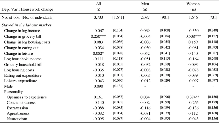
As described by the expression in (2.9), for a person with traits and endowment of effort , actions are also dependent on situations. Following this reasoning, we move to the analysis of the marginal effects of personality traits conditional on each of the two possible situations denoted by : permanence in the labour market, or the occurrence of transition to retirement. Table 5 reports the marginal effects of consumption expenditures, gender and personality traits in each situation. First of all, we observe the positive marginal effect of the personality trait of extraversion on housework at retirement. It shows that for an additional standard deviation on the extraversion score, housework increases 0.959 hours on the top of the effect of a transition to retirement, being stronger and statistically significant for women. Extraversion scores are shown as a more relevant determinant of housework at retirement than consumption expenditures, household income, and gender. This finding is supported by the fact that among the adjectives of extroverted people are pro-active, energetic, and orientated towards people. Extroverted individuals might not be only oriented by productivity, and possibly perceive housework activities, such as cooking for household members and doing grocery shopping, as less costly in terms of effort, or even pleasant. Housework also might allow more extroverted retirees to sustain their pre-retirement levels of leisure and entertainment habits by acting as a substitute for other services that they otherwise would have to pay.
In both the treatment and control groups, changes in household grocery and food weekly bill seem to co-vary positively with weekly hours devoted to housework. This is in line with Luengo-Prado and Sevilla’s (2013) who show that retirees replace some market goods with home-produced goods, mainly in terms of food expenditures.
Changes in net housing costs co-vary positively with housework changes, but only at retirement. Individual leisure expenditures changes co-vary with changes in housework during the individuals’ late years
14
in the labour market. Higher amounts spend on leisure are positively associated with housework changes at retirement. Openness to experience seems to affect the decision of working-aged women about housework. An additional standard deviation in this trait increases housework changes in 0.374 hours. Individuals who are more opened to experience tend to perceive pleasure in low-intensity activities with curiosity about new actions, feelings and ideas.
In sum, these finding support the message that housework operates as an eventual buffer to substitute, by home production, the purchase of market goods and services. By doing housework, individuals are able to spend their monetary income on things that cannot be substituted by home production, such as rent, mortgage payments, or costly leisure activities like travelling and entertainment.
[Table 5]
Figure 2 shows how the effect of a transition to retirement on housework varies for different levels of the statistically significant covariates in Table 5. Higher levels of extraversion determine higher increases in housework hours due to retirement. For example, all else equal, a female with score in extraversion equivalent to the sample average (standardized to zero) has an estimated increase in housework due to retirement of 2.143 hours per week. Another female who has an additional standard deviation on extraversion is estimated to increase her housework at retirement in the order of 3.631 hours per week. Here we can also visualize how housework increases with grocery and food household bill changes and with individual leisure expenditures mainly in the case of female retirees.
The OLS estimation of equation (3.1) includes socio-demographic characteristics as control variables and time-fixed effects, but neither control for permanent unobserved heterogeneity, nor for a potential correlation between a transition to retirement and the transitory error, . Such a correlation arises if housework changes and the decision to retire are determined simultaneously. Furthermore, given the goals of this study, we cannot rely on a larger number of periods after personality traits have been measured. Then, the number of time periods composing our panel, does not allow the implementation of one-way fixed effects estimation without the cost of biased results (Nickell, 1981). The demeaning process embedded in a within estimator of this kind would create a correlation between the regressor of interest and the error term. Other dynamic panel data estimation procedures, such as the ones proposed by Arellano and Bond (1991), Arellano
15
and Bover (1995) and Blundell and Bond (1998) could not be applied in our case because of the absence of valid instruments or the violation of over-identifying restrictions.
The potential outcomes framework described by equation (3.1) seeks to compare the observed housework change of a given individual entering retirement with a counterfactual prediction of housework change if the same retired individual had not in fact entered retirement. Given the fact that no individual can be observed in both situations, the treatment effects literature emphasizes ways to build counterfactuals in observational studies (Cameron and Trivedi, 2006, p. 866). It is possible to match on the propensity score (Heckman, Ichimura and Todd, 1998), which here entails obtaining matched sets of observations of individuals that performed a transition to retirement with observations of individuals who stayed in the labour market. Both sets of observations are then required to have similar probability of entering retirement ( , in a given year and given observed baseline characteristics x: ] (Cameron and Trivedi, 2005, p.864). Matching on propensity scores method allows us to analyse the observational non-randomized data in question by mimicking the characteristics of a non-randomized control trial, and in this sense, reducing selection bias (Austin, 2011, p. 419).
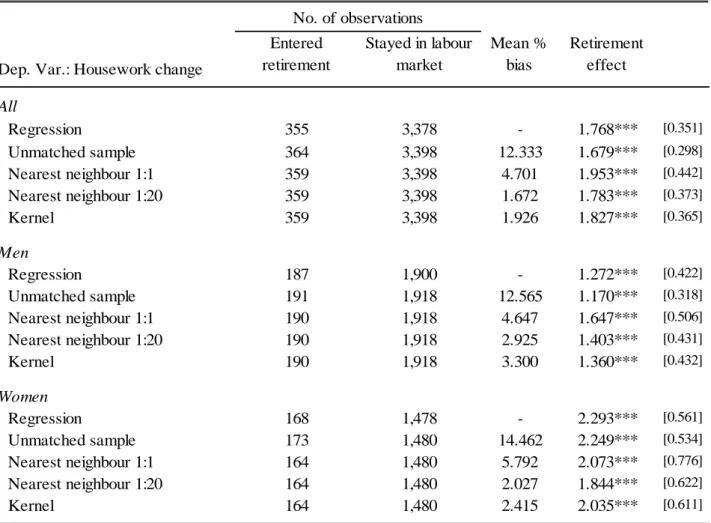
Consequently, we performed a set of matching on propensity score techniques. In order to obtain the corresponding propensity scores, we ran probit estimations with as dependent variable, income, expenditures, age, gender, marital status, income, personality, last job classification, household size, and health status, as baseline covariates.
Table 6 shows the estimated effects of a transition to retirement on housework, according to the following procedures: one-to-one nearest neighbour with no replacement, twenty-to-one nearest neighbours, and kernel. This robustness check validates the estimated impact of retirement obtained with the OLS estimation, with consistent stories also by gender. By analysing the mean percentage bias in the three different estimation methods, we can observe that after the matching both groups are very similar in terms of baseline characteristics, which enhances the argument in favour of the present counterfactual.
[Table 6]
We also assessed the robustness of the conditional marginal effects of personality traits’ results by controlling also for the potential effects of pre-retirement household and individual characteristics observed contemporaneously to personality traits in wave 15. There are a number of factors that may correlate with an
16
individual’s personality traits and that could act as potential confounds or mediators. Hence, we included the as covariates observations in 2005 of log household income, household size, marital status, last job classification, job market status and education. As shown in Table 7, when we controlled for these variables, higher openness to experience scores still predict higher changes in housework conditional on a permanence in the labour market. Also, the more extroverted are still expected to have higher housework increases at retirement.
[Table 7]
5. Conclusion
The action of devoting time to domestic activities and home production of goods and services acts as a substitute for market purchases, a situation which is widely neglected in descriptive models of economic behaviour and decision making at retirement. Here we proposed a two-period model of a transition to retirement that accounts for housework as a component of an individual’s inter-temporal constraint and life-time wealth. Our empirical analysis exploits the empirical advantages of a potential outcomes framework to the estimation of causality in observational (nonrandomized) studies to show that the average retirement effect on housework is positive, for both men and women. We identify extraversion as the key determinant of the changes in the time new retirees devote to these tasks, being more relevant than consumption expenditures, household income, and gender. By address the relationship between non-cognitive skills and retirees’ economic behaviour we contribute to the literature about how older people deal with changes in income and consumption expenditures, and time devoted to domestic activities when they leave the labour market.
17
References
ALMLUND, M., A. DUCKWORTH, J. J. HECKMAN, AND T. KAUTZ, 2011. Personality psychology and economics. In E. A. HANUSHEK, S. MACHIN, AND L. WOSSMANN (Eds.),
Handbook of the Economics of Education, Volume 4. Amsterdam:
Elsevier. Forthcoming.
ARELLANO, M., BOND, S., 1991. Some tests of specification for panel data: Monte Carlo evidence and an application to employment equations. Review of Economic Studies, Volume 58(2), p. 277-297. ARELLANO, M., BOVER, O., 1995. Another look at the instrumental variable estimation of error-components models.
Journal of Econometrics, Volume 68(1), p. 29-51.
AUSTIN, P., 2011. An introduction to propensity score methods for reducing the effects of confounding in observational studies.
Multivariate Behavioral Research, Volume 46(3), p. 399-424.
BANKS, J., BLUNDELL, R., TANNER, S., 1998. Is there a retirement savings puzzle? The American Economic Review, Volume 88 (4), p. 769-788.
BATTISTIN, E., BRUGIAVINI, A., RETTORE, E., WEBER, G., 2009. The retirement consumption puzzle: evidence from a regression discontinuity approach. American Economic Review, Volume 99(5), p. 2209–2226.
BERNHEIM, B., SKINNER, J., WEINBERG, S., 2001. What accounts for the variation in retirement wealth among U.S. households? American Economic Review, Volume 91(4), p. 832–857. BLEKESAUNE, M., SKIRBEKK, V., 2012. Can personality predict retirement behaviour? A longitudinal analysis combining survey and register data from Norway. European Journal of Aging, Volume 1, p. 1-8.
BLUNDELL, R., BOND, S., 1998. Initial conditions and moment restrictions in dynamic panel data models. Journal of Econometrics, Volume 87(1), p. 115-143.
BORGHANS, L., DUCKWORTH, A., HECKMAN, J., WEEL, B., 2008. The economics and psychology of personality traits. Journal of
Human Resources, Volume 43(4), p. 972-1059.
BOYCE, C., WOOD, A., 2011. Personality prior to disability determines adaptation: agreeable individuals recover lost life satisfaction faster and more completely. Psychological Science. Volume 22(11), p. 1397–1402.
BRYAN, M., SEVILLA-SANZ, A., 2011. Does housework lower wages? Evidence for Britain. Oxford Economic Papers, Volume 63(1), p. 187-210.
CAMERON, C., TRIVEDI, P. 2005. Microeconometrics: Methods
and Applications. Cambridge University Press, New York.
CHETTY, R., FRIEDMAN, J., LETH-PETERSEN, S., NIELSEN, T., OLSEN, T., 2012. Active vs. passive decisions and crowd-out in retirement savings accounts: evidence from Denmark. Forthcoming in Quarterly Journal of Economics.
COSTA, P., McCRAE, R., 2006. Age changes in personality and their origins: Comment on Roberts, Walton, and Viechtbauer. Psychological Bulletin, Volume 132, p. 26-28. CRONBACH, J., 1951. Coefficient alpha and the internal structure of tests. Psychometrika, Volume 16(3), p. 297-334.
DIAMOND, P. 1965. National debt in a neoclassical growth model.
American Economic Review, Volume 55, p.1126–1150. Econometrica, vol. 55(3), pp. 533–57.
GOLDSMITH, A., VEUM, J., DARITY, W., 1997. The impact of psychological and human capital on wages. Economic Inquiry, Volume 35, p. 815–829.
GUPTA, S. The effects of transitions in marital status on men´s performance of housework. Journal of Marriage and the Family, Volume 61, p. 700-711.
HAIDER, S., STEPHENS, M., 2007. Is there a retirement-consumption puzzle? Evidence using subjective retirement
expectations. Review of Economics and Statistics, Volume 89(2), p. 247–264.
HAMMERMESH, D., 1984. Consumption during retirement: the missing link in the life-cycle hypothesis. Review of Economics and
Statistics, Volume 66(1), pp. 1-7.
HECKMAN, J., 2011. Integrating personality psychology into economics. NBER Working Papers 17378.
HECKMAN, J., ICHIMURA, H., PETRA, T., 1998. Matching as an econometric evaluation estimator. Review of Economic Studies, Volume 65(2), p. 261-294.
HECKMAN, J. J., J. STIXRUD, S. URZUA, 2006.. The effects of cognitive and noncognitive abilities on labor market outcomes and social behaviour. Journal of Labor Economics, vol. 24 (3), p. 411-482.
HEINECK, G., 2011. Does it pay to be nice? Personality and earnings in the UK. Industrial and Labour Relations Review, Volume 64(5), p. 1020-1038.
HEINECK, G., SILKE, A., 2010. The returns to cognitive abilities and personality traits in Germany. Labour Economics, Volume 17(3), p. 535-546.
HERSCH, J., STRATTON, L., 2002. Housework and wages. Journal
of Human Resources, Volume 37(1), p. 217–229.
HOLM, S., 1979. A simple sequentially rejective multiple test procedure. Scandinavian Journal of Statistics, Volume 6(2), p. 65– 70.
LUENGO-PRADO, M., SEVILLA, A., 2013. Time to cook: Expenditure at retirement in Spain. The Economic Journal, Volume 123, p. 764–789.
MARIGER, R., 1987. A life-cycle consumption model with liquidity constraints: theory and empirical results.
MINIACI, R., MONFARDINI, C., WEBER, G., 2010. Is there a retirement consumption puzzle in Italy? Empirical Economics, Volume 38(5), p. 257–280.
MOEN, P., KIM, J., HOFMEISTER, H., 2001. Couples’ work/retirement transitions, gender, and marital status. Journal of
Social Psychology, Volume 64, No 1, p. 55-71.
NANDI, A., NICOLETTI, C., 2009. Explaining personality pay gaps in the UK. ISER Working Paper Series 2009 (22), Institute for Social and Economic Research.
NICKELL, S., 1981. Biases in dynamic models with fixed effects. Econometrica, Volume 49(6), p. 1417-1426.
ROBB, A. L., BURBIDGE, J., 1989. Consumption, income, and retirement. Canadian Journal of Economics,
SAMUELSON, P. 1958. An exact consumption loan model of interest with or without the social contrivance of money. Journal of
Political Economy, Volume 66, 467–482.
SCHWERDT, G., 2005. Why does consumption fall at retirement? Evidence from Germany. Economics Letters, Volume 89(3), p. 300– 305.
Volume 22(3), p. 522–42.
SPECHT, J., EGLOFF, B., SCHMUKLE, S. C., 2011. Stability and change of personality across the life course: The impact of age and major life events on mean-level and rank-order stability of the Big Five. Journal of Personality and Social Psychology, Volume 101, p. 862-882.
YEE, M., 2008. Does gender trump money? Housework hours of husbands and wives in Britain. Work, Employment & Society, Volume 22, p. 45-66.
YEE, M., 2012. Revisiting the 'doing gender' hypothesis: housework hours of husbands and wives in the UK. In: Understanding society:
findings 2012. Colchester: Institute for Social and Economic
18 FIGURE 1
Average weekly housework hours of employed and retired individuals
0 2 4 6 8 10 12 14 16 18 20 1992 1993 1994 1995 1996 1997 1998 1999 2000 2001 2002 2003 2004 2005 2006 2007 2008 Employed male Employed female Retired male Retired female
19 FIGURE 2
The effects of a transition to retirement conditional on extraversion, grocery bill, and leisure expenditures Extraversion standardized score
Men Women 0.649 0.956 1.262 1.568 1.874 -2.0 -1.0 0.0 1.0 2.0 3.0 4.0 5.0 6.0 7.0 -1.0 -0.5 0.0 0.5 1.0
Mean = -0.493, Std. Dev. = 0.958, 25% = -0.702, Median = -0.137, 75% = 0.429
0.655 1.399 2.143 2.887 3.631 -2.0 -1.0 0.0 1.0 2.0 3.0 4.0 5.0 6.0 7.0 -1.0 -0.5 0.0 0.5 1.0
Mean = 0.021, Std. Dev. = 0.999, 25% = -0.702, Median = 0.146, 75% = 0.712
Change in grocery and food weekly household bill
Men Women 0.958 1.038 1.118 1.198 1.278 -2.0 -1.0 0.0 1.0 2.0 3.0 4.0 5.0 6.0 7.0 -1.0 -0.5 0.0 0.5 1.0
Mean = -0.167, Std. Dev. = 1.347, 25% = -1.000, Median = 0.000, 75% = 1.000
1.637 1.835 2.033 2.231 2.429 -2.0 -1.0 0.0 1.0 2.0 3.0 4.0 5.0 6.0 7.0 -1.0 -0.5 0.0 0.5 1.0
Mean = 0.162, Std. Dev. = 1.326, 25% = -1.000, Median = 0.000, 75% = 1.000
Leisure individual monthly expenses
Men Women 0.523 0.698 0.872 1.046 1.221 1.395 -2.0 -1.0 0.0 1.0 2.0 3.0 4.0 5.0 6.0 7.0 1.0 2.0 3.0 4.0 5.0 6.0
Mean = 3.922, Std. Dev. = 3.109, 25% = 1.000, Median = 3.000, 75% = 6.000
1.151 1.643 2.136 2.629 3.122 3.615 -2.0 -1.0 0.0 1.0 2.0 3.0 4.0 5.0 6.0 7.0 1.0 2.0 3.0 4.0 5.0 6.0
Mean = 2.450, Std. Dev. = 2.296, 25% = 1.000, Median = 2.000, 75% = 3.000
Notes: Descriptive statistics for each variable’s distribution by gender are shown in the top of each chart. Vertical axes indicate the estimated change
in housework hours given a transition to retirement. Horizontal axes denote levels of the corresponding covariate at which eq. (3.1) was estimated. Vertical lines show 90% confidence intervals adjusted for multiple comparisons with the Holm-Bonferroni method (Holm, 1979).
20
Table 1 Summary statistics for housework
Variable (1) (2) (3) (4) (5)
All (No of observ. =11,935)
Housework 11.357 [0.428] 8.949 [0.125] 11.411 [0.102] 2.408*** [0.446] -0.053 [0.440]
Change in housework 1.736*** [0.316] -0.055 [0.087] -0.465*** [0.074] 1.791*** [0.328] 2.202*** [0.324]
No of observations 406 3,718 7,811
Male (No of observ. =5,615)
Housework 7.129 [0.438] 5.175 [0.108] 7.591 [0.116] 1.954*** [0.451] -0.462 [0.454]
Change in housework 1.184*** [0.355] -0.027 [0.088] -0.231** [0.097] 1.211*** [0.366] 1.415*** [0.368]
No of observations 217 2,079 3,319
Female (No of observ. =6,320)
Housework 16.212 [0.600] 13.736 [0.193] 14.233 [0.138] 2.475*** [0.630] 1.979*** [0.615] Change in housework 2.370*** [0.540] -0.090 [0.163] -0.638*** [0.107] 2.460*** [0.564] 3.009*** [0.550] No of observations 189 1,639 4,492 Gender gap Housework -9.083 [0.743] -8.561 [0.221] -6.642 [0.184] -0.522 [0.775] -2.441*** [0.765] Change in housework -1.186*** [0.646] 0.063 [0.186] 0.407*** [0.144] -1.249* [0.682] -1.593** [0.662] No of observations 406 3,718 7,811 Difference 1-3 Stayed retirement Entered retirement Stayed labour market Difference 1-2
Notes: (i) standard errors are shown in the brackets; (ii) columns 1-3 show average housework levels, average changes in housework for each group, and include t-test results for the changes in housework being equal to the null hypothesis; (iii) columns 4 and 5 show t-tests of mean comparisons between groups 1 and 2, and groups 1 and 3, respectively assuming; (iv) all t-tests performed assumed unequal variances; (v) * p< 10%, ** p< 5%, *** p<1%.
21
Table 2 Summary statistics
Log household equivalised annual income 10.077 [0.972] 10.303 [5.311]
Grocery & food weekly household bill (scale 1-12) 6.653 [1.872] 7.250 [2.044]
Log household monthly net housing costs 1.399 [2.391] 2.519 [2.864]
Eating out monthly individual expenditure (scale 0-12) 3.873 [3.088] 4.701 [3.236]
Leisure monthly individual expenditure (scale 0-12) 3.276 [2.866] 3.824 [3.172]
Change in log income -0.111 [0.983] 0.048 [0.710]
Change in grocery bill -0.053 [1.332] 0.104 [1.317]
Change in log housing costs -0.236 [1.573] -0.199 [1.646]
Change in eating out -0.442 [2.577] 0.089 [2.661]
Change in leisure -0.445 [2.746] -0.112 [2.806]
Lagged total household housework 19.828 [10.467] 19.773 [11.481]
Household Size 2.062 [0.738] 2.354 [0.963]
Living with partner/cohabiting 0.800 [0.401] 0.813 [0.390]
Personality (scale 1-7) Openness to experience -0.082 [1.040] 0.018 [0.988] Concientiousness 0.131 [0.977] 0.220 [0.930] Extraversion -0.006 [0.971] -0.155 [0.954] Agreableness 0.094 [0.990] 0.010 [0.969] Neuroticism -0.217 [0.958] -0.188 [0.953] Male 0.527 [0.500] 0.562 [0.496] Age 63.358 [0.505] 59.839 [4.357]
Lagged job market status
Self-employed 0.141 [0.348] 0.193 [0.395]
Employed 0.789 [0.409] 0.787 [0.409]
Unemployed 0.070 [0.256] 0.019 [0.137]
Last job's classification
Professional 0.087 [0.283] 0.054 [0.226]
Manag. & technical 0.307 [0.642] 0.331 [0.471]
Skilled non-manual 0.214 [0.411] 0.224 [0.417] Skilled manual 0.177 [0.383] 0.205 [0.404] Partly skilled 0.152 [0.360] 0.143 [0.349] Unskilled 0.062 [0.241] 0.043 [0.203] Education Degree 0.150 [0.357] 0.138 [0.346] Further 0.090 [0.287] 0.082 [0.274] A-level 0.127 [0.333] 0.182 [0.386] O-level 0.225 [0.418] 0.242 [0.428]
Health status (scale 1-5) 2.130 [0.837] 2.034 [0.774]
No. of observations 355 3,378 No. of individuals 349 1,495 Entered retirement Stayed labour market
Notes: (i) standard deviations are shown in the brackets; (ii) log equivalised household income was obtained by dividing household annual income variable by the household equivalence scale before housing costs (Taylor et al, 2010) provided in the BHPS.
22
Table 3 Domestic division of housework between cohabiting partners per type of activity
Partner does/paid % Baseline Follow-up Baseline Follow-up Men
Grocery shopping 0.534 0.524 0.454 0.333 -0.110*** [0.031]
Cooking 0.678 0.677 0.699 0.623 -0.076** [0.031]
Cleaning/hoovering 0.697 0.707 0.672 0.590 -0.092*** [0.035]
Washing and ironing 0.807 0.817 0.820 0.770 -0.059** [0.029]
No. of observations Women
Grocery shopping 0.098 0.097 0.088 0.051 -0.035 [0.022]
Cooking 0.100 0.092 0.058 0.044 -0.007 [0.023]
Cleaning/hoovering 0.109 0.104 0.117 0.067 -0.045* [0.027]
Washing and ironing 0.048 0.044 0.058 0.000 -0.054** [0.021]
No. of observations
Retirement effect
1,243 137
183
Stayed labour market Entered retirement
1,783
Notes: (i) the table provides the ratio of respondents indicating that his/her partner does most of the indicated household jobs or it is done by paid help/other in the baseline and follow-up period. The BHPS asks couples the following question: Could you please say who mostly does this work here? Is it mostly yourself, or mostly your spouse/partner, or is the work shared equally. The possible responses are: 1 – mostly self, 2 – mostly spouse/partner, 3 – paid help only, 4 – other (specify). We created an indicator variable equal to 1 for responses “mostly spouse/partner” and “paid help only” to measure home division of the corresponding domestic activities: grocery shopping, cooking, cleaning/hovering, and washing/ironing; (ii) retirement effect reported in the last column is calculated as a differences-in-differences estimator, e.g. the difference between the average responses in the group that made a transition to retirement and the group that stayed in the labour market in the follow-up subtracted by the baseline’s period difference between the same groups; (iii) standard error of the retirement effect are shown in brackets; (iv) the difference-in-difference estimator of the retirement effect on individual responses was performed as a t-tests against the null-hypothesis; (v) * p< 10%, ** p< 5%, *** p<1%.
23
Table 4 The effect of a transition to retirement on housework
All Men Woman
Dep. Var.: Housework change (1) (2) (3)
No. of obs. [No. of individuals] 3,733 [1,641] 2,087 [901] 1,646 [731] Transition to retirement 1.768*** [0.351] 1.272*** [0.422] 2.293*** [0.561]
Change in log income -0.119 [0.098] -0.047 [0.092] -0.305 [0.234]
Change in grocery bill 0.266*** [0.081] 0.002 [0.081] 0.548*** [0.148]
Change in log housing costs 0.117** [0.055] 0.017 [0.053] 0.207** [0.106]
Change in eating out -0.025 [0.037] -0.015 [0.040] -0.082 [0.071]
Change in leisure 0.066* [0.037] 0.050 [0.038] 0.088 [0.081]
Log household income 0.007 [0.113] 0.046 [0.112] 0.071 [0.244]
Grocery household bill -0.026 [0.055] 0.003 [0.059] 0.014 [0.105]
Log housing costs -0.050* [0.027] -0.028 [0.028] -0.088* [0.052]
Eating out expenditure -0.013 [0.030] -0.021 [0.030] 0.010 [0.065]
Leisure expenditure -0.025 [0.030] -0.004 [0.029] -0.056 [0.073]
Lagged household housework -0.149*** [0.011] -0.076*** [0.009] -0.308*** [0.021]
Household Size 0.622*** [0.119] 0.151 [0.112] 1.394*** [0.234]
Living with partner/cohabiting 0.898*** [0.248] 0.798** [0.314] 1.152*** [0.423]
Personality Openness to experience 0.107 [0.085] 0.082 [0.093] 0.274* [0.151] Concientiousness -0.089 [0.094] -0.005 [0.099] -0.186 [0.177] Extraversion 0.024 [0.084] -0.057 [0.088] 0.039 [0.153] Agreableness -0.020 [0.085] -0.005 [0.086] 0.105 [0.164] Neuroticism -0.091 [0.085] 0.001 [0.098] -0.063 [0.150] Male 0.054 [0.181] - - - -Age -0.104 [0.244] -0.119 [0.251] -0.500 [0.595] Age squared 0.001 [0.002] 0.001 [0.002] 0.004 [0.005]
Lagged job market status
Self-employed (Ref.)
Employed 0.250 [0.192] 0.102 [0.193] 0.639 [0.428]
Unemployed -0.973 [0.753] -0.543 [0.787] -0.966 [1.479]
Last job's classification
Professional (Ref.)
Manag. & technical -0.242 [0.275] 0.122 [0.254] -0.547 [0.640]
Skilled non-manual -0.297 [0.310] -0.077 [0.302] -0.246 [0.695]
Skilled manual -0.029 [0.314] -0.002 [0.285] 0.835 [0.852]
Partly skilled -0.407 [0.340] -0.437 [0.324] 0.113 [0.757]
Unskilled 0.105 [0.527] 0.191 [0.507] 0.856 [1.044]
24
Table 4 Continued
All Men Woman
Dep. Var.: Housework change (i) (ii) (iii)
Education Degree (Ref.) Further 0.122 [0.299] 0.161 [0.288] -0.051 [0.672] A-level 0.309 [0.228] 0.250 [0.257] 0.152 [0.444] O-level 0.221 [0.238] 0.314 [0.272] 0.157 [0.429] Other 0.331 [0.236] 0.146 [0.274] 0.541 [0.418] Health status Excellent (Ref.) Good 0.262 [0.195] -0.276 [0.229] 0.905*** [0.340] Fair 0.136 [0.255] -0.315 [0.294] 0.820* [0.440] Poor 0.280 [0.562] -0.478 [0.611] 1.540 [0.998] Very poor -0.022 [1.178] 0.095 [1.674] -0.972 [1.431]
Notes: (i) standard errors are shown in the brackets; (ii) All regressions include region and year fixed effects; (iii) * p< 10%, ** p< 5%, *** p<1%.
25
Table 5 Conditional marginal effects of gender, consumption expenditures and personality traits
All Men Women
Dep. Var.: Housework change (i) (ii) (iii)
No. of obs. [No. of individuals] 3,733 [1,641] 2,087 [901] 1,646 [731]
Stayed in the labour mark et
Change in log income -0.067 [0.104] 0.069 [0.108] -0.350 [0.240]
Change in grocery bill 0.250*** [0.084] -0.004 [0.084] 0.508*** [0.152]
Change in log housing costs 0.083 [0.056] -0.006 [0.055] 0.159 [0.110]
Change in eating out -0.034 [0.038] -0.030 [0.042] -0.081 [0.073]
Change in leisure 0.082* [0.078] 0.052 [0.041] 0.140 [0.087]
Log household income -0.111 [0.118] -0.051 [0.115] -0.164 [0.260]
Grocery household bill -0.018 [0.055] -0.032 [0.059] 0.093 [0.106]
Log housing costs -0.035 [0.027] -0.008 [0.028] -0.078 [0.053]
Eating out expenditure -0.010 [0.031] -0.005 [0.030] 0.039 [0.069]
Leisure expenditure -0.043 [0.030] -0.012 [0.029] -0.097 [0.077] Male 0.090 [0.181] - - - -Personality Openness to experience 0.161 [0.087] 0.084 [0.096] 0.374** [0.156] Concientiousness -0.140 [0.095] 0.002 [0.099] -0.265 [0.179] Extraversion -0.088 [0.085] -0.116 [0.089] -0.136 [0.156] Agreableness -0.032 [0.084] -0.081 [0.079] 0.112 [0.168] Neuroticism -0.095 [0.087] -0.004 [0.095] -0.043 [0.156] (Continued)
26
Table 5 Continued
All Men Women
Dep. Var.: Housework change (i) (ii) (iii)
Entered retirement
Change in log income -0.624 [0.424] -0.673 [0.382] -0.899 [1.163]
Change in grocery bill 0.461 [0.259] 0.156 [0.287] 0.904* [0.449]
Change in log housing costs 0.586** [0.210] 0.394** [0.158] 0.698 [0.363]
Change in eating out 0.029 [0.149] 0.131 [0.169] -0.136 [0.259]
Change in leisure -0.096 [0.120] 0.025 [0.120] -0.265 [0.271]
Log household income 0.884 [0.507] 0.646 [0.560] 1.830 [1.059]
Grocery household bill -0.180 [0.242] 0.307 [0.270] -0.780 [0.454]
Log housing costs -0.192 [0.143] -0.222 [0.172] -0.120 [0.227]
Eating out expenditure -0.154 [0.127] -0.194 [0.159] -0.164 [0.224]
Leisure expenditure 0.228* [0.116] 0.163 [0.137] 0.396 [0.268] Male -0.587 [0.813] - - - -Personality Openness to experience -0.169 [0.312] 0.303 [0.388] -0.496 [0.525] Concientiousness 0.605 [0.375] 0.307 [0.514] 0.999 [0.609] Extraversion 0.959*** [0.336] 0.496 [0.386] 1.352** [0.528] Agreableness -0.147 [0.373] 0.005 [0.448] -0.567 [0.636] Neuroticism 0.073 [0.346] 0.323 [0.550] 0.023 [0.515]
Notes: (i) conditional marginal effects were obtained by taking the first derivative of equation (3.1) with respect to each covariate shown in the table, at both situations indicated by { }, stayed in the labour market, , and entered retirement ; (ii) coefficients’ significance tests were adjusted for two comparisons
27
Table 6 Matching on propensity score estimations of effect of a transition to retirement
Dep. Var.: Housework change
Entered retirement Stayed in labour market Mean % bias Retirement effect All Regression 355 3,378 - 1.768*** [0.351] Unmatched sample 364 3,398 12.333 1.679*** [0.298] Nearest neighbour 1:1 359 3,398 4.701 1.953*** [0.442] Nearest neighbour 1:20 359 3,398 1.672 1.783*** [0.373] Kernel 359 3,398 1.926 1.827*** [0.365] Men Regression 187 1,900 - 1.272*** [0.422] Unmatched sample 191 1,918 12.565 1.170*** [0.318] Nearest neighbour 1:1 190 1,918 4.647 1.647*** [0.506] Nearest neighbour 1:20 190 1,918 2.925 1.403*** [0.431] Kernel 190 1,918 3.300 1.360*** [0.432] Women Regression 168 1,478 - 2.293*** [0.561] Unmatched sample 173 1,480 14.462 2.249*** [0.534] Nearest neighbour 1:1 164 1,480 5.792 2.073*** [0.776] Nearest neighbour 1:20 164 1,480 2.027 1.844*** [0.622] Kernel 164 1,480 2.415 2.035*** [0.611] No. of observations
Notes: (i) the table reports the retirement effect obtained in each matching on propensity scores method; (ii) in order to obtain the propensity scores in each estimation, we ran probit models that had S as dependent variable, and as covariates: male, personality scores, and lagged (baseline) measures of age, squared age, household housework, log equivalised income, grocery and food bill, housing costs, leisure and eating out individual expenditures, whether cohabiting with spouse or partner, household size, education, job class, job market status and year(wave); (iii) the matching on propensity scores estimator of the retirement effect on individual housework works as a difference in difference estimator, i.e. it subtracts the average change in housework hours of the group of observations that made a transition to retirement to the average change of group that stayed in the labour market; (iv) to test the significance of the corresponding estimators, t-tests against the null-hypothesis were performed; (v) * p< 10%, ** p< 5%, *** p<1%.
28
Table 7 Conditional marginal effects of gender, consumption expenditures and personality traits
All Men Women
Dep. Var.: Housework change (i) (ii) (iii)
No. of obs. [No. of individuals] 3,648 [1,606] 2,040 [891] 1,608 [705]
Stayed in the labour mark et
Openness to experience 0.142 [0.088] 0.047 [0.098] 0.371** [0.158] Concientiousness -0.167 [0.098] -0.009 [0.100] -0.321 [0.183] Extraversion -0.079 [0.087] -0.107 [0.094] -0.131 [0.158] Agreableness -0.026 [0.086] -0.061 [0.082] 0.131 [0.172] Neuroticism -0.100 [0.088] 0.001 [0.096] -0.014 [0.159] Entered retirement Openness to experience 0.006 [0.310] 0.365 [0.381] -0.107 [0.503] Concientiousness 0.523 [0.389] 0.115 [0.542] 0.750 [0.613] Extraversion 1.015*** [0.338] 0.435 [0.409] 1.358** [0.523] Agreableness 0.014 [0.395] 0.092 [0.493] -0.233 [0.705] Neuroticism 0.097 [0.325] 0.183 [0.566] -0.154 [0.489]
Notes: (i) in this robustness check we included as covariates the observations of log household income, household size, marital status, last job classification, job market status and education, in 2005, the same year/wave that personality traits have been measured; (ii) conditional marginal effects were obtained by taking the first derivative of equation (3.1) with respect to each covariate shown in the table, at both situations indicated by { }, stayed in the labour market, , and
entered retirement ; (iii) coefficients’ significance tests were adjusted for two comparisons with the Holm-Bonferroni method (Holm, 1979); (iv) standard errors are shown in the brackets; (v) * p< 10%, ** p< 5%, *** p<1%.