© 2000Kluwer Academic Publishers. Printed in the Netherlands. 155
Analysis of the deep chlorophyll maximum across the Azores Front
M. F. Macedo
1, P. Duarte
2∗, J. G. Ferreira
1, M. Alves
3& V. Costa
31Department of Environmental Sciences & Engineering, Faculty of Sciences and Technology, New University of Lisbon, P-2825 Monte de Caparica, Portugal
2Department of Sciences & Technology, Fernando Pessoa University, Praça 9 de Abril 349, P-4249-004 Porto, Portugal (∗author for correspondence)
3Department of Oceanography and Fisheries, University of Azores, 9900 Horta, Portugal
Received 13 September 2000; in revised form 23 September 2000; accepted 24 Ocober 2000
Key words:deep chlorophyll-amaximum, primary production, nutricline
Abstract
Physical, chemical and biological observations made in late July and August 1997 across the Azores Front (37◦ N, 32◦W to 32◦N, 29◦W) are presented. The objectives of the study were: (1) to analyse horizontal and vertical profiles of temperature, salinity, density, nutrients and chlorophyll-a(Chla) of the top 350 m; (2) to identify the main differences in the deep ChlaMaximum (DCM) and hydrographic structure between the water masses that pass north and south of the Azores Front; and (3) to estimate phytoplankton primary production in these water masses. Horizontal and vertical profiles of salinity, temperature, density, nutrients and phytoplankton pigments in the top 350 m were analysed. The Front separates two distinct water types: the 18◦C Mode Water (18 MW) of sub-tropical origin, and the 15◦C Mode Water (15 MW) of sub-polar origin. Differences in the DCM and hydrographic structure between 18 MW and 15 MW were observed in the contour plots of each section. The average Chla
concentration between 5 and 200 m depth decreased significantly from 15 MW to 18 MW. The same pattern was observed for the Chlaconcentration at the DCM depth. A vertical one-dimensional model was used to estimate the phytoplankton primary production in the 15 MW and 18 MW and led to an estimated water column average gross primary productivity (GPP) between 1.08 and 2.71 mg C m−3d−1for the 15 MW and about half of these values for the 18 MW. These results indicate that the typical south–north positive slope on DCM depth parallels a latitudinal increase on GPP, suggesting that the location of the Azores Front may have a significant regional impact on GPP.
Introduction
Fronts are relatively narrow regions characterised by large horizontal gradients in variables such as tem-perature, salinity and density, and by eddy formations like rings and large-scale gyres. These physical struc-tures can affect nutrient levels in the euphotic zone and, thereby, greatly modify the pattern of phytoplank-ton primary productivity of such areas. Many frontal zones are reported as areas of enhanced biological activity (Holligan, 1981; Kahru & Nommann, 1991).
The deep chlorophyll maximum (DCM) is a well-documented phenomenon in several ocean regions. It is a permanent feature in the sub-tropical oligotrophic
con-sequences of DCM formation over relatively short distances.
Several mechanisms have been proposed to explain DCM formation. An increase in the amount of Chl
a per cell in shade-adapted cells at low light levels rather than a real increase of phytoplankton biomass has been suggested as a possible explanation (Cul-len, 1982; Taguchi et al., 1988). The accumulation of sinking cells at depths with high vertical stability created by pycnoclines or a decrease in the sink-ing rate of cells (Bienfang et al., 1983; Takashi & Hori, 1984) has also been related to the appearance of a DCM. Other authors argue that phytoplankton behaviour (Kamykowsky, 1980) and changes in graz-ing pressure between different layers (Kononen et al., 1998) may contribute significantly to the DCM.
The main objective of this paper was to analyse the DMC across the FCA in summer situation. To achieve this goal it was necessary: (1) to analyse the horizontal and vertical profiles of temperature, salin-ity, denssalin-ity, nutrients and Chl a of the top 350 m; (2) to identify the main differences in the DCM and hydrographic structure between the water masses that pass north and south of the Azores Front; and (3) to estimate phytoplankton primary production in these water masses.
Description of the study site
The Azores Archipelago is located in the mid-Atlantic ridge between 35◦and 40◦N. The FCA, south of the Azores Archipelago (Figure 1), is a permanent feature throughout the year and it forms part of the sub-tropical North Atlantic gyre (Klein & Siedler, 1989; Alves et al., 1994). It appears as a southern branch of the Gulf Stream that splits at the Grand Banks of New-foundland. North Atlantic Central Water constitutes the main body of the FCA, whereas Mediterranean Water occupies its bottom end (Alves, 1996). The FCA is also seen as the boundary between 18◦C (to the South) and 15◦C (to the North) mode Waters (15 MW and 18 MW). Associated with the Azores Front are strong horizontal thermohaline gradients that can be easily located both at the surface and at depth with temperature data alone (Siedler & Zenk, 1985). Gould (1985) found that the Front could be identified most readily by the position of the 16◦C isotherm at a depth of 200 m.
Figure 1. Generalised topography of the North Atlantic basin (mod-ified from Gould (1985)). The location of the surveyed area is represented in a rectangle together with the aproximate location of the Azores Front at the time of survey.
Materials and methods
Sampling program
Between 19th July and 5th August, 1997, an intens-ive cruise was carried out onboard R/VArquipélago
(Arquipélago Research Vessel) involving CTD meas-urements (Aquatracka III fluorometer, Chelsea In-struments), in situ fluorometric measurements and water sampling. Four parallel transepts and one cross-transept were performed from 37◦N 32◦15′W to 32◦ N 29◦W (Figure 2). The four parallel transepts will be designated here as sections 1, 2, 3 and 4, from left to right. The geographic distribution of the transepts was chosen to allow the characterisation of the wa-ter masses that cross the Azores Front. A total of 52 CTDs were made. The mean distance between CTD sampling stations was about 37 km. At each station, water samples were collected at fourteen depths (about 1000, 850, 700, 550, 350, 250, 200, 150, 100, 80, 60, 40, 20 and 0 m) for salinity, Chla and nutrient de-terminations (nutrient and pigment samples were only collected at 10 depths in the top 350 m). In the present work, only results between 0 and 350 m depth are ana-lysed, because these are the most relevant regarding primary productivity and DCM.
Analytical methods
Figure 2. The position of the CTD sampling stations. Also shown are the contours of the depth of the 16◦C isotherm. The bold line corresponds to the location of the FCA, separating 15 MW to the north and 18 MW to the south (see text).
using an EVOLUTION II autoanalyser, at the Dept. of Oceanography and Fisheries, University of Azores. Samples for the determination were filtered onboard using 0.45µm (∅47 mm) membrane filters. The filters were frozen and subsequently chlorophyll extracted with 90% acetone. Chlaand phaeopigment concentra-tion were determined fluorometrically by the method of Yentsch & Menzel (1963) as modified by Holm-Hansen et al. (1965). The fluorescence measurements were performed in a SPEX Fluorolog F111 that was first calibrated with pure Chla(Sigma Chemical). For the fluorometer Aquatracka III calibration curve, only values above 0.01 mg Chl a m−3 were considered because this is the lower limit of the Aquatracka III detection range. The relation between Chlaand fluor-escence did not change significantly over the sampling period and a single calibration curve was fitted to all data. The calibration curve obtained by non-linear regression was:
Chla−0.0112(±0.0003)×e1.8890(±0.00198)×F (1)
where chlorophyll is given in mg m−3 and F is the
output of the fluorometer in Volts. Chl a
concentra-tion values, as well as all CTD data, were interpolated for every 1 m using the Kriging method (Press et al., 1985).
Statistical analysis
The differences in the DCM and hydrographic struc-ture between the surveyed areas – North and South of the front (15 and 18MW, respectively) (cf. Figure 2) – were investigated by means of analysis of variance (ANOVA) (Sokal & Rohlf, 1995). Since the location of the stations in both areas was not chosen at ran-dom during the sampling campaign, they could not be treated as replicates. Therefore, one subgroup of sta-tions to the North and another to the South (6 stasta-tions in both cases) were chosen at random for statistical analysis. Prior to ANOVA, variance homogeneity was checked by the tests of Cochram, Hartley and Bartlett (Underwood, 1981). The relationship of the means and variances was also inspected. Data were transformed in the case of variance heterogeneity or a significant relationship between means and variances.
For each station the parameters investigated were defined as follows:
1. DCM depth – depth of the deep Chl amaximum (m),
2. Chlamax – Chlaaconcentration maximum (mg Chlam−3),
3. N2at the DCM – stability of the water column at the DCM depth (s−2),
4. σθ at the DCM – density (σθ) at the depth of chlorophyll maximum (kg m−3),
5. DCM width – Vertical extension for which the chlorophyll concentration is always above 0.1 mg Chlam−3(m),
6. Chl a average – Average Chl a concentration between 5 and 200 m (mg m−3),
7. Depth N2max – Depth of the stability maximum between 5 and 100 m. This is an estimate of the depth of the seasonal pycnocline (m),
8. Nitrate – average nitrate concentration in the top 200 m (mmol m−3),
9. Nitrite – average nitrite concentration in the top 200 m (mmol m−3),
10. Silicate – average silicate concentration in the top 200 m (mmol m−3),
Average concentrations were calculated from val-ues of the top 200 m since these are the most relevant regarding DCM.
Description of the model
A vertical one-dimensional model was used to estim-ate the phytoplankton primary production in the north and south areas. Sixty-three vertical layers were con-sidered, each with 4 m depth, to simulate a 252 m water column. The model was implemented using an object-oriented programming (OOP) approach by means of the EcoWin software (Ferreira, 1995; Duarte & Ferreira, 1997).
Light intensity (I) was used as a forcing function for primary productivity. Estimation of I and radi-ation fluxes between the ocean and the atmosphere were calculated from latitude and date using standard formulations described in Brock (1981) and Portela & Neves (1994). The light extinction coefficient (k
in m−1) was calculated as a function of the Chl a
concentration by means of Equation 2 (Parsons et al., 1984). k was used to calculate the Photosynthetic-ally Active Radiation (PAR) available for each vertical layer.
k=0.04+0.0088.Chla+0.054.Chla2/3. (2)
The model described in Eilers & Peeters (1988, 1993) was used to simulate primary productivity (Plight
in mg C mg Chla−1h−1) as a function of PFD (µmol
photons m−2s−1).
Plight= I
aI2+bI+c. (3)
This model was chosen because it is based on the physiology of photosynthesis and its depth integration equation has an analytical solution (Eilers & Peeters, 1988). By differentiating the Eilers & Peeters (1988) model as a function of light, the parameters initial slope (αin mg C mg Chla−1h−1µmol photons m2 s1), optimal I (Ioptµmol photons m−2 s−1) and max-imal productivity (Pmax in mg C mg Chl a−1 h−1) (Eilers & Peeters, 1988) of the production-light re-lation can be expressed as a function of a, b andc
parameters:
α=1
c. (4)
Iopt= r
c
a. (5)
Pmax=
1
b+2√ac. (6)
Nitrogen was considered as the limiting nutrient in the model following other authors (e.g Fasham et al., 1990), and its effect on phytoplankton growth rate was included by means of a Michaelis–Menten formulation (Parsons et al., 1988):
PN=Plight N Ks+N
, (7)
wherePN is the nutrient (nitrate nitrogen) and light limited productivity, N is the nitrate concentration (mmol m−3) in water andKsis the half-saturation
con-stant for nitrate uptake. There were no data available for ammonia concentration, therefore solely nitrate limitation was considered in the simulations. Silicate was not considered in this model since most of the primary production in the DCM in this area is due to cyanobacteria (Platt et al., 1983). The influence of the temperature on the production rate (P) was described by a formulation based on Eppley (1972):
P +P Nea×T, (8)
wherea is the temperature augmentation rate andT
is the water temperature in◦C. Respiration was com-puted as a fixed fraction (respiration coefficient) of primary production during daylight and as a fixed rate (maintenance respiration) of the phytoplankton bio-mass during the night. Phytoplankton biobio-mass and nitrate concentrations were considered constant dur-ing the simulation time. Chlorophyll concentrations were assumed constant during the simulation period, because the objective of the model was exclusively to calculate primary production for a short period of time, integrating light intensity variation and nitrate concentration variability over the water column. Exud-ation was calculated as a constant fraction of the gross primary production. Mortality and sinking rates were not considered in this model.
Table 1 presents the parameter values used in the model simulations. With the exception of latitude and
Ks (half-saturation for nitrate uptake) all paramet-ers were considered constant and equal in 15 MW and 18 MW. Different Ks values were tested to in-vestigate the influence of nitrate limitation on the production rates. The parameters of the production– light curve were selected within the range of those measured by Platt et al. (1983) for the Mid-Atlantic Ridge west of the Azores (0.24–1.0 mg C mg Chl
Table 1. Parameters used in the model simulations
Parameter name Unit Value
a(temperature augmentation rate) ◦C 0.069
Maintenance respiration % of biomass 2
Respiration Coefficient % of production 10
Exudation rate % of production 5
Carbon/Chlorophyll ratio mgC mgChla−1 32
Pmax(maximal production rate) mgC mgChla−1h−1 0.57
α(initial slope) mgC mgChla−1h−1µE−1m2s 0.10 Iopt(optimal light intensity) µE m−2s−1 87.4 Ks(half-saturation for Nitrate uptake) mmol m−3 0–2
Latitude ◦ 34.5 for 15 MW
32.0 for 18 MW
h−1 µmol photons−1 m2s1 for α and 60–70 µmol
photons m−2s−1 forIopt). The carbon/chlorophyll
ra-tio used in the model was chosen from the rara-tios measured by Irwin et al. (1983) in the vicinity of the Azores Front. The temperature augmentation rate was taken from Dippner (1997). All these parameter values are well within the ranges reported in the literature (see Parsons et al., 1984; Jørgensen et al., 1991).
The model simulations were carried out to analyse the primary production in 15 MW and 18 MW, during a summer situation. Mean vertical profiles of nitrate, phytoplankton biomass and water temperature, cal-culated from thein situ measurements, were used to set the initial conditions for model simulations. The model time step used was 1 h and all the simulations were performed between Julian Day 202 and 206, in order to reproduce summer conditions.
Results
The results presented here are divided into five sec-tions. The first and second parts are mainly a descrip-tion of the physical oceanography of the study area and the hydrographic structure of the top 350 m, respect-ively. In the third part, the mean profiles of nutrient concentration between 15 MW, Front and 18 MW are compared, followed by the statistical analysis of the differences in DCM and hydrographic structure between 15 and 18 MW in the fourth part. Finally, the phytoplankton primary production in the 15 MW and 18 MW is investigated using the model described above.
Figure 3. Typicalθ- S curves (potential temperature - salinity) for 18 MW (station 51) and 15 MW (station 20).
General physical oceanography of the area
Figure 2 shows the CTD sampling stations and the depth of the 16◦C isotherm. The approximate position of the Front can be determined by the 16◦C isotherm at a depth of 200 m accordingly to Gould (1985). Dur-ing this study, the 16◦C isotherm was found around 150 m in the north and went deeper to the south down to 300 m (Figure 4).
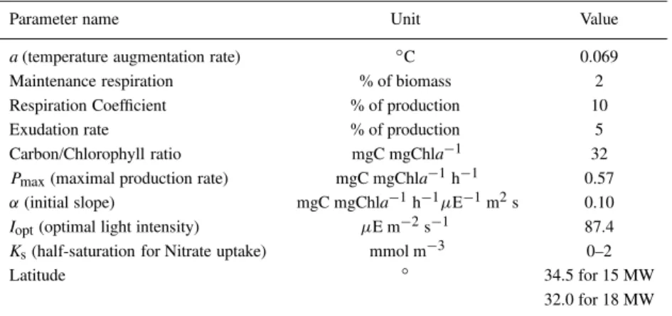
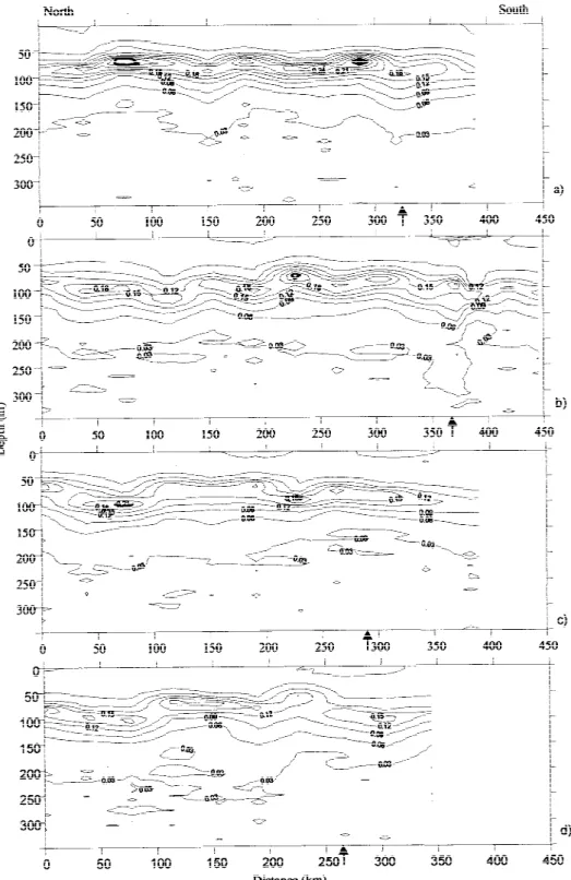
Figure 4. Contoured sections of potential temperature (contour interval 1◦C) of the top 350 m of the water column for the 4 sections: (a) section 1; (b) section 2; (c) section 3; (d) section 4. The arrows mark the position of the Front detected by the fast deepening of the isotherms between 14 and 17◦C.
in 18 MW(32.3◦N; 31.6◦W) and another located in 15 MW (34.3◦N; 31◦W), plotted in Figure 3.
Both water masses presented a similar θ–S rela-tionship between 11 and 15◦C, but at higher temper-atures the 15 MW was consistently less saline. The
at greater depths (temperature lower than 8◦C), both water types again showed the sameθ–S relationship.
Hydrographic structure of the top 350 m
The CTD data from the four sections described above was analysed to highlight some important features of the spatial distribution of Chl a and its relationship with the physical structure of the top 350 m of the water column. (Figures 4–6).
The main features of the temperature structure in the upper 350 m of the surveyed area can be seen in Figure 4. The northern part of each section was typified by the 14◦C and 16◦C isotherms being al-ways above 300 and 150 m respectively, and by the absence of water warmer than 24◦C at the surface. In the southern part, the 16◦C isotherm sank below 300 m and the surface water became warmer in this area. The position of the Front was easily observed by the fast deepening of the isotherms between 17◦C and 14◦C. A thermocline with about 3◦C of variation was observed between 15 and 35 m in the north area, with a thin mixed layer in the top. The thermocline was found deeper in the south area between 25 and 50 m, with a mixed layer located in the first 20–25 m. A well marked thermostad below the seasonal ther-mocline (between 100 and 250 m) with a temperature close to 15◦C was observed in the north area, defining the 15 MW main structure. In the south, a thermostad involving 18◦C water of subtropical origin was also detected.
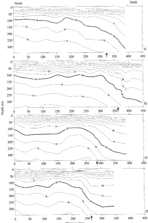
Contoured sections of salinity for the four sections are presented in Figure 5. The 36.1 isohaline was al-ways above 200 m in the northern part of each section and below 300 m in the southern part. The observed surface salinity values in the 18 MW were higher than in the 15 MW. The frontal zone was very well recog-nised by the deepening of the isohalines and by the stability of the salinity values in the top 150 m of the water column.
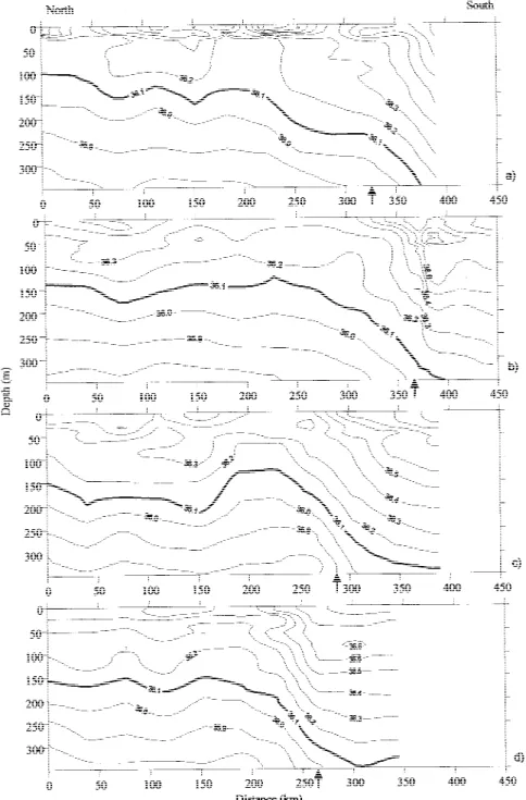
The transition between the north and south water bodies was also clearly seen in the vertical sections of density (σθ) by the deepening of the 26.4, 26.6 and 26.8 isopycnals (Figure 6). The 26.6 isopycnal was always shallower than 150 m in the north part and went deeper than 200 m in the southern area. In fact, the 26.6 and 26.7 isopycnals appeared to follow the 16◦C isotherm very closely (cf. Figures 4 and 6). The seasonal pycnocline was observed around 25 m in the 15 MW and deeper, around 40 m, in the 18 MW.
The Chlaconcentration ranged from less than 0.04 to 0.3 mg Chla m−3, but it was always lower than
0.05 mg Chla m−3 in the top 25 m (Figure 7). The
DCM in the 18 MW was deeper and with lower Chl
aconcentration than those of the 15 MW. The highest concentration values were observed between 60 and 90 m in the north and between 90 and 110 m in the south area (cf. Figure 10). The Chl a concentration decreased to values lower than 0.05 mg Chl a m−3 below 150 m.
Mean profiles of nutrient concentrations
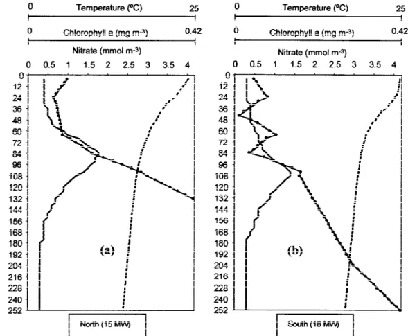
Another factor that can affect the formation and main-tenance of the DCM is the nutrient concentration. Vertical profiles of nitrate, nitrite, phosphate and silic-ate concentrations for 15 MW, Front and 18 MW are presented in Figures 8 and 9.
Mean nitrate mean concentration for the first 350 m of the surveyed areas ranged from 0.18 to 9 mmol m−3. Nitrate concentrations in the south were lower than those in the north and Front areas, except between 200 and 350 m when the south and Front wa-ters showed the same concentrations. Within the first 100 m of the surveyed area, nitrate profiles presented a high degree of variability. Nevertheless, it was pos-sible to observe a nitracline located between 60 and 100 m; the north and Front areas have a very similar nitrate concentration in this depth interval.
Nitrite concentration ranged from 0 to 0.105 mmol m−3 and presented a completely different vertical
profile from the nitrate, with higher values located between 60 and 100 m.
Mean phosphate concentration for the first 350 m ranged from 0.03 to 1.04 mmol m−3(Figure 9). In the Front zone, a maximum in the phosphate tion occurred in the surface water. Lower concentra-tion values in the north and Front areas were observed between 20 and 80 m.
Mean silicate concentration ranged from 0.23 to 3.5 mmol m−3(Figure 9). Silicate concentration was higher in the 15 MW than in the 18 MW, with the Front showing intermediate values. The lowest silic-ate values, for the three surveyed areas, were observed between 20 and 80 m.
Figure 5. Contoured sections of salinity (contour interval 0.1) of the top 350 m of the water column for the 4 sections: (a) section 1; (b) section 2; (c) section 3; (d) section 4. The arrows mark the position of the Front.
presenting minimum values between 50 and 100 m depth, which corresponds approximately to the DCM depth.
Statistical analysis of the differences in the DCM and hydrographic structure between 15 MW and 18 MW.
AN-Figure 6. Contoured sections of density (contour interval 0.2 kg m−3) of the top 350 m of the water column for the 4 sections: (a) section 1; (b) section 2; (c) section 3; (d) section 4. The arrows mark the position of the Front.
OVA results for the differences between values in 15 and 18 MW. Mean values for the frontal zone were found to be intermediate in magnitude between the 15 MW and 18 MW, with only three exceptions for the DCM width and Phosphate average that presented
Figure 7. Contoured sections of chlorophyll-aconcentration (contour interval 0.03 mg Chlam−3) of the top 350 m of the water column for the 4 sections: (a) section 1; (b) section 2; (c) section 3; (d) section 4. The arrows marks the position of the Front.
differences between 15 MW and 18 MW regarding the DCM and hydrographic structure are:
Figure 8. Mean vertical profiles±2 SE of nitrate (a) and nitrite (b) concentration for north (15 MW), Front and south (18 MW).
(ii) The water density at the depth of the DCM was significantly higher in the 15 MW;
(iii) The vertical extent of DCM (measured by DCM width) was about 20 m greater in 15 MW than in 18 MW;
(iv) The average Chl a concentration between 5 and 200 m and the Chla max decreased from 15 MW to 18 MW, and was significantly differ-ent between those two areas;
(v) (The seasonal pycnocline (Depth N2max) was
on average 19 m deeper in 18 MW than in 15 MW;
(vi) Nitrate and silicate mean concentration values of the top 200 m were found lower in 18 MW than in 15 MW.
Phytoplankton primary production – results of the model simulations
The results from the previous sections showed signi-ficant differences in the DCM depth and magnitude between the 15 MW and 18 MW, as well as significant differences in nitrate and silicate mean concentrations
Figure 9. Mean vertical profiles±2 SE of phosphate (a) and silicate (b) concentration for north (15 MW), Front and south (18 MW).
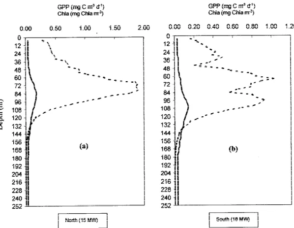
of the top 200 m. The model was elaborated as simply as possible, to investigate the differences in phyto-plankton primary production between 15 MW and 18 MW and to analyse the effect of nitrate limitation. The mean values used to initialise the model (Fig-ure 10) clearly show that the DCM, for both areas, was found near the nitracline and below the thermocline.
The vertical profiles of light intensity simulated for either side of the Front showed no significant differ-ences. Although this was expected, since only 2.5◦ of latitude separated those areas, the lower chloro-phyll of the 18 MW (Figure 11b) could have allowed a deeper light penetration in this area. Actually, chloro-phyll values in both areas were so low that the water particles were the main contributors to the average ex-tinction coefficient. These results imply that absolute light levels played a minor role in determining the dif-ferences in the chlorophyll vertical profiles between those two areas.
Vertical profiles of GPP (mg C m−3d−1) predicted
pro-Figure 10. Vertical profiles of the model initial values for 15 MW (a) and 18 MW (b): temperature (broken line), nitrate concentration (solid line with circles) and Chlaconcentration (solid line).
duction calculated for 18 MW (73 mg C m−2d−1). For
15 MW, the GPP profile followed the Chlaprofile ob-served: the peak of primary production coincides with the chlorophyll maximum. For the 18 MW, the model predicts two peaks of GPP: one around the DCM depth and another around 64 m. This second peak in primary production is a consequence of the increase of nitrate in this layer (cf. Figure 10), but it is unrelated with the Chlaprofile observed in the south area.
Six model runs were performed using three differ-entKs values (0, 1 and 2) to investigate the effect of nitrate limitation for each area (Figure 12). According to these results, the maximal GPP in 15 MW ranged from 1.08 mg to 2.71 mg C m−3 d−1, whereas the
maximal GPP values achieved in 18 MW were about half of these values – 0.52–1.51 mg C m−3 d−1. In both cases the minimal values were obtained with a
Ks of 2. The variation inKs influenced the GPP val-ues in both areas but it only affected the shape of the GPP mean vertical profile in the 18 MW; this was
be-cause of the low nitrate concentration at 84 m depth in 18 MW. This low value explains the low GPP in all 18 MW simulations except those with no nutrient lim-itation. In a non-limiting situation for nitrate, the south area has its GPP maximum between 50 and 110 m, but in a strong nitrate limitation scenario (withKs=2) the GPP presents 2 peaks, one at around 100 m and another at around 64 m.
According to these results, a maximum specific growth rate ranging from 0.27 (under nutrient limit-ation) to 0.85 d−1(without nutrient limitation) can be achieved in both areas between 50 and 60 m depth, by dividing GPP by average phytoplankton biomass. Somewhat lower maximal growth rates were observed in the same area by other authors – 0.1–0.18 d−1(Platt et al., 1983; Fasham et al., 1985). These results indic-ate that the optimal layer for growth is locindic-ated above the DCM, both in 15 MW and 18 MW.
Figure 11. Vertical profiles of daily average gross primary production (GPP) (broken line) and its relation with the Chlaprofile (solid line) for 15 MW (a) and 18 MW (b). These results were obtained withKs= 0.5.
depth, defined as the depth where the net photosyn-thesis averaged over the day is zero, is located below the DCM depth, around 120–130 m, in both areas. Therefore, considering the whole euphotic zone, car-bon fixation ranging from 47.1 to 131.5 mg C m−2d−1 could be achieved in 15 MW and values from 26.4 to 103.2 mg C m−2 d−1could be found in 18 MW, depending on the nitrate limitation, by integration of the simulated GPP values over depth. The maximum values predicted for each area were calculated based on the assumption of no nutrient limitation (Ks = 0), therefore, these values correspond to the maximal net production that can be achieved in those areas, using these mean Chlaprofiles, if light and temperature are the only limiting factors.
In the oligotrophic ocean, the vertical eddy diffus-ivity is normally low, of the order of 0.3×10⁻⁴m2 s−1(Mann & Lazier, 1996). Using this value and the nitrate gradient observed in the vicinity of the DCM for 15 MW and 18 MW (cf. Figure 10), it was possible to infer how much new production could be supplied
by the nitrate flux through the nutricline. Therefore, with a nitrate gradient of 0.05 mmol N m−3m−1and 0.015 mmol N m−3m−1for 15 MW and 18 MW, re-spectively, an upward nitrate flux of 1.81 mg N m−2 d−1 and 0.54 mg N m−2 d−1 was estimated . As-suming a C:N ratio of 6.6 (Parsons et al., 1988), this converts to a carbon fixation of 11.95 mg C m−2d−1 and 3.56 mg C m−2 d−1 for 15 MW and 18 MW, respectively. These values fall in the range of those calculated by Lewis et al. (1986) for the oligotrophic Atlantic Ocean, Southeast of Azores. These authors calculated an eddy diffusivity of 0.37×10⁻⁴m2s−1
and a mean vertical flux of 1.96 mg N m−2d−1. These
Figure 12. Vertical profiles of daily average gross primary production (GPP), for 15 MW (a) and 18 MW (b), predicted by the model using 3 different values ofKs.Ks= 0 (broken line);Ks= 1 (line with squares);Ks= 2 (solid line).
in a summer situation, which calculated anfaverage annual value of 0.7, with a winter maximum approach-ing 0.8–0.9 and a summer minimum reachapproach-ing almost 0.1–0.2.
Discussion
In the results presented, the Azores Front was found to be separating two distinct water bodies, the 18 MW to the south, and the 15 MW to the North. The frontal boundaries between the two water types were more sharply defined by salinity than temperature (cf. – Fig-ures 4 and 5). Fasham et al. (1985) hypothesised that the reason for this is that horizontal differences in tem-perature structure are more susceptible to modification by interaction with the atmosphere than differences in salinity. For both areas, a DCM was found near the nitracline and below the seasonal pycnocline and thermocline. The DCM in the 18 MW was on average 20 m deeper than in 15 MW, and the nitrate and silic-ate mean concentration for the top 200 m was found
lower in the 18 MW. Since seasonal pycnocline was on average 19 m deeper in the south, one possible explan-ation for the deeper DCM observed in this area could be that the seasonal pycnocline was created earlier in the south, so that at the time of the survey the DCM would be at a later stage and, therefore, deeper than in the north area. These observations are in agreement with the downward slope of the DCM from the sub-Arctic towards the subtropics observed by Strass & Woods (1991). However, the slope estimated from the data presented here is about the double than the one measured by those authors between the Polar Front and Azores.
Table 2. Mean value and standard deviation of the parameters describing the DCM and hydrographic structure of the water column, for the three areas (15 MW, Frontal zone and 18 MW). ANOVA results for the differences between the 15 MW and 18 MW are also presented
Parameter 15 MW Front 18 MW ANOVA results
DCM depth (m) 81.3±12.6 94.1±10.8 103.5±5.6 p<0.001 Chlamax (mg m−3) 0.23±0.04 0.18±0.02 0.15±0.03 p<0.05 N2at DCM (s−2×10⁻⁵) 5.71±4.68 3.70±4.12 3.38±2.41 No significant differences
σθat DCM (kg m−3) 26.47±0.04 24.42±0.06 26.37±0.01 p<0.01 DCM width (m) 45.7±5.8 55.3±15.6 28.9±7.0 p<0.001 Chlaaverage 7.7±0.8 7.7±1.1 6.2±0.5 p<0.001 (mg m−3×10⁻²)
Depth N2max (m) 22.3±10.5 30.6±9.0 41.3±5.6 p<0.001 Nitrate (mmol m−3) 2.15±1.08 1.80±0.67 1.09±0.40 p<0.05 Nitrite (mmol m−3) 0.04±0.04 0.04±0.01 0.03±0.02 No significant differences Silicate (mmol m−3) 0.97±0.42 0.67±0.23 0.54±0.27 p<0.05 Phosp. (mmol m−3) 0.17±0.06 0.24±0.21 0.13±0.1 No significant differences
Table 3. Mean values of several parameters determined for the Azores Front by Fasham et al. (1985) and the present study (ranges including minimal and maximal values without distinction between 15 and 18 MW)
Parameter Spring Summer
(April and May, 1981) (July–August, 1997) Fasham et al. (1985) Present study
DCM depth (m) 61–89 81.3–103.5
Chlamax (Chlaconcentration 0.34–0.41 0.15–0.23 maximum - mg Chlam−3)
Depth N2max - Seasonal pycnocline 35–48 22–41 depth (m)
Maximum growth rate (d−1) 0.10–0.18 0.23–0.85 Upward nitrate flux (mg N m−2d−1) 1.2 (EAW) 0.54–1.81
comparison, two major differences can be pointed out. Firstly, the DCM depth observed in this study was on average 20 m deeper than the one found by Fasham et al. (1985) in the spring (April and May, 1981). This deepening in the DCM corresponds to about 8 m per month and it is in agreement with the range of 7.5– 10 m per month determined by Strass & Woods (1991) for the oligotrophic north Atlantic during the heating season. Secondly, the maximum Chlavalues observed in the present study were about half of the ones re-ported by Fasham et al. (1985), as was expected in a summer situation with a deeper DCM.
Small differences between these studies were ob-served in the seasonal pycnocline, maximal specific growth rate and upward nitrate flux (Table 3). Note that Fasham et al. (1985) calculated only the upward
nitrate flux for the Eastern Atlantic Water, located northeast of the Azores Front, so this value can only be compared with the upward nitrate flux estimated for the north area in the present study.
ob-served proximity of the DCM and the nutricline depth appear to agree well with the models of Jammart et al. (1977, 1979) and Wolf & Woods (1988). Those models predict a progressive descent of the DCM dur-ing the oligotrophic conditions in summer followdur-ing the deepening of the nutricline. It is likely that after a certain point the light intensity received by the cells is very low, leading to a slow growth and slow nitrogen depletion.
The estimated upward vertical nitrate flux of 1.81 mg N m−2 d−1 and 0.54 mg N m−2 d−1 for 15 MW and 18 MW, respectively, indicate that new production in the south (18 MW) is about 30% of the new production that could be achieved in the north area (15 MW). These results could explain the lower Chlaconcentration found in 18 MW and stress the im-portance of considering the upward nutrient flux when modelling the DCM in this area.
Other factors which may be responsible for (or contribute to) the DCM formation and maintenance, and that were not considered in the model should also be considered. Steele & Henderson (1992) emphas-ised the importance of predation in plankton models. Grazing by herbivorous zooplankton could contribute to the DCM if differential grazing between layers was considered. On the other hand, the deeper and less pronounced DCM observed in the 18 MW could also be explained by a higher grazing pressure in this area. Angel (1989) studied the vertical profiles of pelagic communities (macroplankton and micronekton) in the vicinity of the Azores Front. He found sharp declines in the standing-crops of both plankton and micronek-ton from the Eastern Atlantic Water, located north of the Front, to the Western Atlantic Water, south of the Front. Based on these results Fasham et al. (1985) considered that for the vicinity of the Azores Front, an explanation based on the differential grazing was un-likely. Furthermore, Cullen (1982) showed that most of the vertical profiles of chlorophyll could be accoun-ted for by other processes without special regard for grazing. More recently, in the South Atlantic, White-house et al. (1996) observed a significant removal of phytoplankton biomass that could not be explained by zooplankton grazing. However, pelagic communities can also affect the DCM indirectly due to their vertical migrations. As Angel (1989) pointed out, migrating plankton can play an important role in the active trans-port of organic substances down from the euphotic zone and in redistributing nutrients across the nutri-cline. Longhurst & Harrison (1988) estimated that up to 25% of the nitrogen utilized by the phytoplankton
in the euphotic zone is exported below the nutricline by migrants, which suggests that the impact of plank-ton migrations on the transport of organic substances and nutrient distributions should be taken into account, especially in the water column is stable.
Although sinking rate was not considered in the present model, there are reasons to believe that this is not one of the major factors affecting the DCM depth in this area. The results of Bienfang et al. (1983) in-dicate that there is no need to use the sinking rate to explain the DCM in oligotrophic subtropical oceans, where phytoplankton cells are small and the response to decreasing light is sufficient to account for the ob-served increase in chlorophyll with depth, throught changes in the C:Chlaratio. Jamart et al. (1979) also showed by means of sensitivity analysis, that changes in sinking rate were not important in their model. More recently, Varela et al. (1992) also found that sink-ing factors did not seem to affect the predicted DCM structure.
In the present work, C:Chlaratio was considered constant and equal for both 15 MW and 18 MW. How-ever, it is known that this relationship is highly vari-able and can change with temperature, daily irradiance and nutrient concentration (Cloern et al., 1995; Geider et al., 1997), since phytoplankton tend to adapt their C:Chla ratio to the prevailing environmental condi-tions. There is also evidence that sometimes a vertical profile of chlorophyll does not represent phytoplank-ton biomass profile (Cullen, 1982; Taylor et al., 1997). Therefore, an effort should be made when studying the DCM structure, to estimate the phytoplankton carbon profile and its relationship with the Chlaprofile.
Conclusions
The important differences in primary productiv-ity between the water masses separated by the front, suggest that its location may have a very important im-pact on north Atlantic primary productivity and there-fore on the gas exchanges at the ocean–atmosphere interface.
Acknowledgements
This research was supported by PRAXIS XXI Pro-gram (PhD grant 4/4.1/BD/4146) and by project “Nu-merical simulation of climate variability of the Açores Front/Current System. Impact on primary production.” (3/3.2/EMG/1956/95). The authors acknowledge the comments of two anonymous reviewers which greatly improved the manuscript. The helpful discussions and laboratory facilities provided by F. J. Pina are also acknowledged.
References
Alves, M. A., A. Simões, A. C. De Verdiére & M. Juliano, 1994. Atlas Hydrologique Optimale pour l’Atlantique Nord-Est et Centrale Nord (0◦–50◦W, 20◦–50◦N). Université des Açores, 76 pp.
Alves, M., 1996. Dynamic instable d’un Jet Subtropical. Le cas du systéme Fron-Courant des Açores. PhD thesis at the “Université de Bretagne Occidentale-Laboratoire de Physique des Oceans”, Brest, France: 229 pp.
Aminot A. & M. Chaussepied, 1983. Manuel des analyses chimiques en milieu marin. Centre national pour l’exploration des océans (CNEXO). Brest, France: 395 pp.
Angel, M. V, 1989. Vertical profiles of pelagic communities in the vicinity of the Azores Front and their implications to deep ocean ecology. Prog. Oceanogr. 22: 1–46.
Bienfang, P. K., J. Syper & E. Laws, 1983. Sinking rate and pigments responses to light-limitation of marine diatom: implica-tions to dynamics of chlorophyll maximum layers. Oceanol. Acta 6: 55–62.
Brock, T. D., 1981. Calculating solar radiation for ecological studies. Ecol. Model. 14: 1–19.
Cloern, J. E., C. Grenz & L. Videgar-Lucas, 1995. An empirical model of the phytoplankton chlorophyll:carbon ratio – the con-version factor between productivity and growth rate. Limnol. Oceanogr. 40: 1313–1321.
Cullen, J. J., 1982. The deep chlorophyll maximum: comparing vertical profiles of chlorophylla. Can. J. Fish. aquat. Sci. 39: 791–803.
Dippner, J. W., 1993. A lagrangian model of phytoplankton growth dynamics for the Northern Adriatic Sea. Cont. Shelf Res. 13: 331–355.
Duarte, P. & J. G. Ferreira, 1997. Dynamic modelling of photosyn-thesis in marine and estuarine ecosystems. Env. Model. Assess. 2: 83–93.
Eberlein K. & G. Kattner, 1987. Automatic method for the determ-ination of orthophosphate and total dissolved phosphorus in the marine environment. Fres. Z. Anal. Chem. 326: 354–357.
Eilers, P. H. C. & J. C. H. Peeters, 1988. A model for the rela-tionship between light intensity and the rate of photosynthesis in phytoplankton. Ecol. Model. 42: 199–215.
Eilers, P. H. C. & J. C. H. Peeters, 1993. Dynamic behaviour of a model for photosynthesis and photoinhibition. Ecol. Model. 69: 113–133.
Eppley, R. W., 1972. Temperature and phytoplankton growth in the sea. Fish. Bull. 70: 1063–1085.
Fasham, M. J. R., T. Platt, B. Irwin & K. Jones, 1985. Factors affecting the spatial pattern of the deep chlorophyll maximum in the region of the Azores Front. Prog. Oceanogr. 14: 129–165. Fasham, M. J. R., H. W. Ducklow & S. M. McKelvie, 1990. A nitrogen-based model of plankton dynamics in the oceanic mixed layer. J. mar. Res. 48: 591–639.
Ferreira, J. G., 1995. ECOWIN – An object-oriented ecological model for aquatic ecosystems. Ecol. Model. 79: 21–34. Geider R. J., H. L. MacIntyre & T. M. Kana, 1997. A dynamic
model of phytoplankton growth and acclimation: responses of balanced growth rate and the chlorophylla:carbon ratio to light, nutrient limitation and temperature. Mar. Ecol. Prog. Ser. 148: 187–200.
Gould, W. J., 1985. Physical oceanography of the Azores Front. Prog. Oceanogr. 14: 167–190.
Holligan, P. M., 1981. Biological implications of Fronts on the north-west European continental shelf. Phil. Trans. r. Soc., Lond., Series A, 302: 547–562.
Holm-Hansen, O., C. J. Lorenzen, R. W. Holmes & J. D. H. Strick-land, 1965. Fluorometric determination of chlorophyll. Journal du Conseil, Conseil permanent International pour l’Exploration de la Mer 30: 3–15.
Irwin, B., T. Platt, P. Lindley, M. J. Fasham & K. Jones, 1983. Phytoplankton Productivity in the vicinity of a Front S.W. of the Azores during May, 1981. Can. Data Rept. Fish. aquat. Sci. 400: 101 pp.
Jammart, B. M., D. F. Winter, K. Banse, G. C. Anderson & R. K. Lam, 1977. A theoretical study of phytoplankton growth and nutrient distribution in the Pacific Ocean of the northwest U. S. coast. Deep Sea Res. 24: 753–773.
Jammart, B. M., D. F. Winter & K. Banse, 1979. Sensitivity analysis of a mathematical model of phytoplankton growth and nutrient distribution in the Pacific Ocean of the northwest U. S. coast. J. Plankton Res. 1: 267–290.
Jørgensen, S. E., S. N. Nielsen & L.A. Jørgensen, 1991. Handbook of ecological parameters and ecotoxicology. Elsevier, London: 840 pp.
Kahru, M. & S. Nommann, 1991. Particle (plankton) size structure across the Azores Front (Joint Global Ocean Flux Study North Atlantic Bloom Experiment). J. Geophys. Res. 96 (C4): 7083– 7088.
Kamykowsky, D., 1980. Sub-thermocline maximum of the dino-flagellatesGymnodinium simplex(Lohmann) Kofoid and Swezy and Gonyaulax polygrammma Stein. Northeast Gulf Sci. 4: 39–43.
Klein, B. & G. Siedler, 1989. On the origin of the Azores Current. J. Geophys. Res. 94 (C5): 6159–6168.
Kononen, K., S. Hällfors, K. Marjaana, H. Kuosa, J. Laanemets, J. Pavelson & R. Autio, 1998. Development of a subsurface chloro-phyll maximum at the entrance to the Gulf of Finland, Baltic Sea. Limnol. Oceanogr. 43: 1098–1106.
Longhurst, A. R. & W. G. Harrison, 1988. Vertical nitrogen flux from the oceanic photic zone by diel migrant zooplankton and nekton. Deep Sea Res. 35: 881–889.
Mann, K. H. & J. R. N. Lazier, 1996. Dynamics of marine ecosys-tems. Biological-physical interactions in the oceans. 2nd Edn. Blackwell Science, Massachusetts, U.S.A., 394 pp.
Parsons, T. R., M. Takahashi & B. Hargrave, 1984. Biological Oceanographic Processes. Pregamon Press, New York: 233 pp. Platt, T., D. V. Subba Rao & B. Irwin, 1983. Photosynthesis of
picoplankton in the oligotrophic ocean. Nature 301: 702–704. Press, W. H., S. A. Teukolski, W. T. Vetterling & B. P. Flannery,
1995. Numerical recipes in C – The art of scientific computing. Cambridge University Press, Cambridge, 924 pp.
Portela, L. I. & R. Neves, 1994. Modelling temperature distribu-tion in the shallow Tejo estuary. In Tsakiris & Santos (eds), Advances in Water Resources Technology and Management. Balkema, Rotterdam: 457–463.
Siedler, G. & W. Zenk, 1985. Strong currents events related to a subtropical Front in the Northeast Atlantic. J. Phys. Oceanogr. 15: 885–897.
Sokal, R. R. & F. J. Rohlf, 1995. Biometry: the principles and prac-tice of statistics in biological research. 3rd edn. W.H. Freeman and Company, New York, U.S.A., 887 pp.
Steele, J. H. & E. W. Henderson, 1992. The role of predation in plankton models. J. Plankton Res. 14: 157–172.
Strass, V. H. & J. D. Woods, 1991. New production in the sum-mer revealed by the sum-meridional slope of the deep chlorophyll maximum. Deep Sea Res. 38: 35–56.
Strickland, J. D. H. & T. R. Parsons, 1972. A practical handbook of seawater analysis. 2nd edn. Fish. Res. Bd. Can. Bulletin 167, Ottawa: 311 pp.
Taguchi, S., G. R. Ditullio & E. A. Laws, 1988. Physiological characteristics and production of mixed layer and chlorophyll maximum phytoplankton populations in the Caribbean Sea and western Atlantic Ocean. Deep Sea Res. 35: 1363–1377. Takashi, M. & T. Hori, 1984. Abundance of picophytoplankton in
the subsurface chlorophyll maximum layer in subtropical and tropical waters. Mar. Biol. 79: 177–186.
Taylor, A. H., R. J. Geider & F. J. H. Gilbert, 1997. Seasonal and latitudinal dependencies of phytoplankton carbon–chlorophylla ratios: results of a modelling study. Mar. Ecol. Prog. Ser. 152: 51–66.
Underwood, A. J., 1981. Techniques of analysis of variance in experimental marine biology and ecology. Oceanogr. mar. biol. Ann. Rev. 19: 513–605.
Varela, R. A., A. Cruzado, J. Tintoré & E. G. Ladona, 1992. Modelling the deep- chlorophyll maximum: a coupled physical-biological approach. J. mar. Res. 50: 441–463.
Whitehouse, M. J., J. Priddle, P. N. Trathan & M. A. Brandon, 1996. Substantial open-ocean phytoplankton blooms to the north of South Georgia, South Atlantic during summer 1994. Mar. Ecol. Prog. Ser. 140: 187–197.
Wolf, K. U. & J. D. Woods, 1988. Lagrangian simulations of primary production in the physical environments – the deep chlorophyll maximum and nutricline. In Rothschild, B. J. (ed), Toward a Theory on Biological-Physical Interations in the World Ocean. Kluwer Academic Publishers: 51–70.