April| 2017
Pedro Emanuel de Gouveia Alonso
MASTER IN APPLIED BIOCHEMISTRY
Alternative Methods for the Synthesis
of Electrically Conductive Bacterial Cellulose-polyaniline
Composites for Potential Drug Delivery Application
Pedro Emanuel de Gouveia Alonso
MASTER IN APPLIED BIOCHEMISTRY MASTER DISSERTATION
Alternative synthesis methods of electrically conductive
bacterial cellulose-polyaniline composites for potential
drug delivery application
Tese apresentada à Universidade da Madeira com vista à obtenção do grau de Mestre em
Bioquímica Aplicada
Pedro Emanuel de Gouveia Alonso
Sob a orientação de:
Professora Doutora Nereida Maria Abano Cordeiro
Faculdade de Ciências Exatas e da Engenharia
Universidade da Madeira
Funchal – Portugal
I
Acknowledgments
The accomplishment of this Master Thesis was only possible with the help of several
people who I am truly grateful for them being part of my daily life.
I would like to thank Prof. Dr. Nereida Cordeiro for the guidance, support, share of
ideas and constructive critics which were crucial to make this work possible.
I would also give a big thank you to my work colleagues Marisa Faria, Igor Fernandes
and Tomásia Fernandes for pushing me out of my comfort zone and for helping me being
the person I am today. A special hug to Marisa Faria for being a mentor and for giving me
the knowledge and support that made this work possible to conclude.
I am grateful to Prof. Dr. Gabriel Gomes (Physics Department, University of
Madeira, Portugal) for creating the electrical conductivity measurement system, by the
availability shown, as also by clarifying any doubts regarding the measurements.
I want to acknowledge the help provided by the laboratory technicians Paula Andrade
and Paula Vieira for providing the reagents as also to laboratory technician Adriano Faria
for providing me the laboratory equipment and space for the antimicrobial measurements.
I would like to thank Dr. Carla Miguel (CQM, University of Madeira, Portugal) by
providing me help with the contact angle measurements as also to Prof Dr. Paula Castilho
(CQM, University of Madeira, Portugal) for providing me the ATR accessory.
I would like to thank Prof. Dr. Manuela Gouveia (University of Madeira, Portugal)
for providing me the Eschericia coli (E. coli) strain as also the conditions to make the experiment
successful.
I am truly grateful to prof Dr. Artur Ferreira (CICECO, University of Aveiro,
Portugal) for making the TGA and XRD analysis, to Prof. Dr. Faranak Mohammadkazemi
(New Technologies and Energy Engineering, Shadid Beheshti University, Iran) for the EDX
analysis and for Dr. Matic Resnik (Department of Surface Engineering and Optoelectronics,
Jožef Stefan Institute, Slovenia) for the AFM analysis, which substantially increased the
quality of the current Master Thesis.
I want to give a big hug to my friends Magda Santos, Lisandra Sousa, Paulo Costa,
Anísia Martins, Dina Maciel and Micael Leça for the support and motivation during this
II Gouveia for the unconditional love, support and care throughout my entire existence, which
made me possible to get up to this point in life.
III
Abstract
Bacterial cellulose/polyaniline (BC/PANi) nanocomposites have been lately
receiving attention by the scientific community towards the development of electronic
applications. The current work aims to determine the most suitable BC modification method
to obtain an effective drug delivery membrane through electric stimulus. Thus, the BC/PANi
nanocomposites were synthesized through the employment of different BC matrixes
(drained, freeze dried and regenerated), as well as through different polymerization methods
(in situ and ex situ). Prior to modification, the effects of both drying methods (freeze drying
and oven drying), and regeneration process on BC structure were studied. By freeze drying
BC, the fibril network is preserved, leading to a more porous material. On the other hand,
regenerated BC presented a compact surface due to the incapacity to reorganize into fibrils
during the regeneration process. This way, freeze dried BC should be more suited for
modification. To obtain a highly conductive nanocomposite, the in situ polymerization on
drained BC should be employed. The introduction of PANi onto BC obstructed the pores,
which led into a more compact and rougher material. Also, a decrease in the thermal stability,
as well as a decrease in the BC crystallinity was observed. The nanocomposites were drug
loaded with sodium sulfacetamide to evaluate the antimicrobial activity. It was observed that
without electrical stimulus, only drug loaded drained in situ BC/PANi nanocomposite
presented an inhibitory effect onto the Escherichia coli (E. coli) growth (13%). By applying
electric stimulus onto this membrane, the inhibition in E. coli growth is further evidenced
(20%). This way, in situ polymerization of aniline on drained BC presented to be an effective
method to create a highly conductive membrane for drug release through electrical stimulus.
Keywords: Bacterial cellulose, Polyaniline, cellulose modification, antimicrobial activity,
V
Resumo
Os nanocompósitos de celulose bacteriana/polianilina (CB / PANi) têm recebido nos
últimos tempos um grande interesse por parte da comunidade científica para o
desenvolvimento de aplicações eletrónicas. Este trabalho tem como objetivo determinar o
método de modificação mais adequado da CB para a obtenção de uma membrana eficaz na
libertação de fármacos através de estímulo elétrico. Assim sendo, os nanocompósitos
CB/PANi foram sintetizados utilizando diferentes matrizes de CB (drenada, liofilizada e
regenerada) bem como através de diferentes métodos de polimerização (in situ e ex situ). Antes
da modificação, foram estudados os efeitos tanto do método de secagem (liofilização e
secagem no forno) como também o processo de regeneração na estrutura da CB. O processo
liofilização levou à preservação da estrutura tridimensional, obtendo assim um material mais
poroso. Por outro lado, a CB regenerada apresentou uma superfície compacta devido à
incapacidade de reorganizar-se em fibrilas durante o processo de regeneração. Desta forma,
a CB liofilizada aparenta ser a matriz mais adequada para modificação. Contudo,
relativamente aos diferentes nanocompósitos obtidos, para se obter uma membrana com
elevada condutividade, o método mais adequado é a polimerização in situ na CB drenada. A
introdução de PANi na CB obstruiu os poros, levando à formação de um material mais
compacto e rugoso. Também foi observado uma diminuição na estabilidade térmica bem
como uma diminuição na cristalinidade da CB. A sulfacetamida de sódio foi incorporada
nos nanocompósitos para avaliar a atividade antimicrobiana onde, sem estímulo elétrico,
apenas o nanocompósito in situ com CB drenada apresentou um efeito inibitório sobre o
crescimento de Escherichia coli (E. coli) (13%). Através da aplicação de estímulo elétrico sobre
esta membrana, a inibição no crescimento de E. coli é potenciado (20%). Assim sendo, a
polimerização in situ da anilina numa membrana drenada mostrou ser eficaz na libertação
do fármaco por estímulo elétrico.
Palavras-chave: celulose bacteriana, polianilina, modificação da celulose, atividade
VII
Index
Alternative synthesis methods of electrically conductive bacterial cellulose-polyaniline
composites for potential drug delivery application ... I
Acknowledgments ... I
Abstract ... III
Resumo... V
Index ... VII
Figure captions ... XI
Table captions ... XIII
List of abbreviations ... XVII
Chapter I – Introduction ... 1
1.1 – Cellulose ... 1
1.1.1 – Bacterial cellulose ... 2
1.2 – Cellulose modification ... 4
1.2.1 –Cellulose dissolution ... 5
1.2.2 – Intrinsically Conductive Polymers ... 7
1.3 –Inverse Gas Chromatography ... 11
1.3.1 – IGC instrumentation ... 12
1.3.2 – Surface energy ... 13
1.3.2.1 – Dispersive component ... 13
1.3.2.2 – Specific component ... 14
1.3.3 – Acid-base character through Gutmann Method ... 15
1.3.4 – Surface nanomorphology ... 15
1.3.5 –Surface area ... 16
1.3.6 – Surface Heterogeneity ... 17
1.3.7 – Diffusion analysis ... 17
1.3.8 – Work of adhesion ... 18
Aim of the study ... 19
Chapter II – Materials and methods ... 21
2.1 – BC production ... 21
2.2 – BC dissolution optimization ... 21
2.3 – BC nanocomposites synthesis ... 22
VIII
2.4 – Drug loading capacity ... 25
2.5 – Antimicrobial Activity ... 25
2.6 – Statistical analysis ... 26
2.7 – Characterization methods ... 27
2.7.1 – Attenuated total reflectance Fourier transformed infrared spectroscopy ... 27
2.7.2 – X–ray diffraction ... 27
2.7.3 – Thermogravimetrical analysis ... 28
2.7.4 – Scanning electronic microscopy coupled with energy dispersive X–ray spectroscopy ... 28
2.7.5 – Atomic force microscopy ... 28
2.7.6 – Electrical conductivity measurement ... 29
2.7.7 – Swelling capacity ... 30
2.7.8 – Contact angle measurement ... 30
2.7.9 – Inverse Gas Chromatography ... 31
Chapter III – Results and discussion ... 33
3.1 – Influence of bacterial cellulose drying routes and regeneration on its final properties ... 33
3.1.1 – BC regeneration ... 33
3.1.2 – Structural properties ... 35
3.1.2.1 – Fourier transformed infrared spectrometer coupled to attenuated total reflectance 35 3.1.2.3 – X-ray dispersive spectroscopy ... 36
3.1.2.4 – Thermogravimetrical analysis ... 38
3.1.3 – Morphological properties ... 40
3.1.3.1 – Scanning electronic microscopy and atomic force microscopy ... 40
3.1.4 – Swelling and contact angle analysis ... 42
3.1.5 –Surface properties by IGC ... 43
3.1.5.1 – Surface energy ... 43
3.1.5.2 – Acid–base surface character ... 45
3.1.5.3 – Surface nanomorphology ... 48
3.2 – Influence of the different BC modification towards the synthesis of conductive BC/PANi nanocomposites ... 51
3.2.1 – Structural properties ... 51
IX
3.2.1.4 – Thermogravimetrical analysis ... 56
3.2.2 – Morphological properties ... 58
3.2.2.1 – Scanning electronic microscopy and atomic force microscopy ... 58
3.2.3 – Polymer uptake and Electrical conductivity ... 61
3.2.4 – Swelling and contact angle analysis ... 62
3.2.5 – Surface properties by IGC... 65
3.2.5.1 – Surface energy ... 65
3.2.5.2 – Acid-base surface character ... 68
3.2.5.3 – Surface nanomorphology ... 70
3.3 – Application of BC/PANi nanocomposites for potential drug delivery system ... 73
3.3.1 – Work of adhesion and drug loading... 73
3.3.2 – Antimicrobial activity... 74
Chapter IV – Conclusion ... 79
XI
Figure captions
Figure 1 – Schematic representation of cellulose Iα (-), Iβ (-) crystalline structures (based from (10)).
... 2
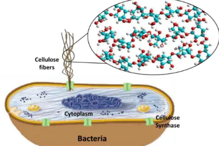
Figure 2 – Schematic representation of BC assembly (based from (19)). ... 3
Figure 3 – Schematic representation of the interactions established between cellulose and DMAc/LiCl (based from (48)). ... 7
Figure 4 –Schematic representation of doped PANi π–system (A) and diagram demonstrating the energy gap (Eg) between metal, semiconductor and isolators (B) ... 9
Figure 5 – Reaction mechanism representation of aniline polymerization through chemical
oxidation ... 10
Figure 6 – Schematic representation of the inverse gas chromatographer apparatus. ... 12
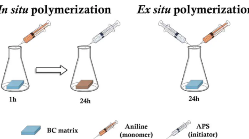
Figure 7 – Schematic representation of the methodology employed for in situ and ex situ PANi polymerization. ... 24 Figure 8 - Schematic representation of the methodology employed for the in situ aniline
polymerization during BC regeneration... 24
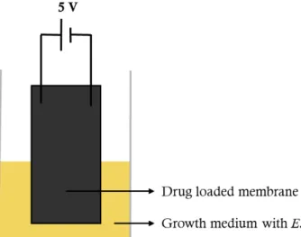
Figure 9 – Schematic representation of the experimental set-up for the drug release through
electrical stimulus. ... 26
Figure 10 – Schematic representation of the 4–probe resistivity measurement principle ... 30
Figure 11 – Dissolution of BC in DMAc/LiCl prior to dissolution (A) and after dissolution(B). ... 34 Figure 12 – Photomicrography (100x) of unoptimized BC dissolution (A) and optimized BC
dissolution (B) in DMAc/LiCl. ... 34
Figure 13 – FTIR–ATR spectra of oven dried (OD–BC), freeze dried (FD–BC) and regenerated (R– BC) BC. ... 36
Figure 14 – X–ray diffraction profile of oven dried (OD–BC), freeze dried (FD–BC) and regenerated (R–BC) BC. ... 37
Figure 15 – Thermogravimetrical analysis (TGA and dTGA (inset)) of the oven dried (OD–BC), freeze dried (FD–BC) and regenerated (R–BC) BC. ... 39
Figure 16 – SEM micrographs (3000x) of oven dried (OD–BC), freeze dried (FD–BC) and
regenerated (R–BC) BC. ... 40
Figure 17 – 3D–and 2D–AFM of oven dried (OD–BC (A, D)), freeze dried (FD–BC (B, E)) and regenerated (R–BC (C, F)) BC. ... 41
Figure 18 – Swelling behaviour of oven dried (OD–BC), freeze dried (FD–BC) and regenerated (R– BC) BC. ... 42 Figure 19 – Contact angle analysis of oven dried (OD–BC), freeze dried (FD–BC) and regenerated (R–BC) BC. ... 43
Figure 20 – Heterogeneity profile of n–octane on oven dried (OD–BC), freeze dried (FD–BC) and regenerated (R–BC) at 25 ºC. ... 45
Figure 21 – Specific free energy of adsorption (ΔGSSP) of the polar probes on oven dried (OD–BC), freeze dried (FD–BC) and regenerated (R–BC) BC. ... 46
Figure 22 – Heterogeneity profile of ethanol (A) and tetrahydrofuran (B) on oven dried (OD–BC), freeze dried (FD–BC) and regenerated (R–BC) BC AT 25 ºC. ... 47
XII
Figure 26 – Thermogravimetrical analysis (TGA and dTGA (inset)) of drained (A), freeze dried (B)
and regenerated (C) BC/PANi nanocomposites. ... 57
Figure 27 – SEM micrographs (3000x) of BC matrixes and BC/PANi nanocomposites ... 59
Figure 28 – 3D–AFM of BC matrixes and BC/PANi nanocomposites... 60
Figure 29 – Swelling behaviour of BC/PANi nanocomposites. ... 62
Figure 30 – Contact angle analysis of the BC matrixes and BC/PANi nanocomposites. ... 64
Figure 31 – Surface energy measurements obtained at 25 ºC from BC matrixes and BC/PANi nanocomposites. ... 66
Figure 32 – Heterogeneity profile of n–octane from BC matrixes and BC/PANi nanocomposites at 25 ºC... 67
Figure 33 –Heterogeneity profile of ethanol (A) and tetrahydrofuran (B) from the BC/PANi nanocomposites at 25 ºC.. ... 68
Figure 34 – Specific free energy of adsorption (ΔGSSP) of polar probes onto the BC/PANi nanocomposites at 25 ºC ... 69
Figure 35 – Antimicrobial activity of the membranes determined through the optical density method at 600 nm. ... 75
XIII
Table captions
Table 1 – Dissolution parameters tested on BC dissolution. ... 22
Table 2 – Physical constants of the applied probes in IGC. ... 32
Table 3 – Crystallinity index (CI), crystallite size (CrS), Z value, and cellulose II/I ratio of oven dried (OD–BC), freeze dried (FD–BC) and regenerated (R–BC) BC. ... 37
Table 4 – Swelling maximum (SWmax) and contact angle of oven dried (OD–BC), freeze dried (FD– BC) and regenerated (R–BC) BC. ... 42
Table 5 – Surface energy (γSD, γSSPand γSTotal,) and acid/base behaviour (ethanol/tetrahydrofuran ΔGSSP ratio and Kb/Ka) of oven dried (OD–BC), freeze dried (FD–BC) and regenerated (R–BC) BC at 25 ºC. ... 44 Table 6 –Surface area (SBET), diffusion parameter (Dp) and morphology indexes of oven dried (OD– BC), freeze dried (FD–BC) and regenerated (R–BC) BC. ... 49
Table 7 – Energy dispersive X–ray spectroscopy data of the BC matrixes and BC/PANi
nanocomposites. ... 53
Table 8 – Crystallinity index (CI), and Temperature maximum (Tmax) obtained through XRD and TGA analysis, respectively, for the BC matrixes and BC/PANi nanocomposites. ... 55 Table 9 – Polymer content and electrical conductivity of the BC/PANi nanocomposites. ... 62
Table 10 – Swelling maximum (SWmax) and contact angle of the BC matrixes and BC/PANi
nanocomposites. ... 63
Table 11 – Surface energy (γSD and γSSP, γSTotal) and acid/base behaviour (Kb/Ka and
ethanol/tetrahydrofuran ΔGSSP ratio) of BC/PANi nanocomposites at 25 ºC. ... 65
Table 12 – Surface area (SBET), diffusion parameter (Dp) and morphology indexes from the BC matrixes and BC/PANi nanocomposites at 25 ºC. ... 71
XVII
List of abbreviations
∆𝑮𝒔𝒅–Surface Gibbs free energy of the dispersive component ∆𝑮𝒔𝒔𝒑– Surface Gibbs free energy of the specific component
γLD– Liquid surface tension
𝛄𝐒−– Donor number of the probe 𝛄𝐒+ – Acceptor number of the probe
𝛄𝐒𝐃– Dispersive component of the surface energy 𝛄𝐒𝐒𝐏–Specific component of the surface energy 𝛄𝐒𝐓𝐨𝐭𝐚𝐥– Total surface energy
∆𝑮𝒂𝑴– Distance between the probe and the alkane line
13C NMR– Carbon–13 nuclear magnetic ressonance
A – Adsorption potential
am–Cross section area of the probe molecule
FTIR–ATR –Fourier transformed infrared coupled withattenuated total reflectance
BC –Bacterial cellulose
CI –Crystallinity index
CrS –Crystallite size
DMAc– Dimethylacetamide
dTGA –Derivative of TGA
EDX – Energy dispersive X–ray spectroscopy
ES –Oven dried BC/PANi nanocomposite obtained through ex situ polymerization
F– Carrier gas (helium) flow rate
FD–BC– Freeze dried bacterial cellulose
FD–ES –Freeze dried BC/PANi nanocomposite obtained through ex situ polymerization
FD–IS –Freeze dried BC/PANi nanocomposite obtained through in situ polymerization
FID– Flame ionization detector GC– Gas chromatography
H – Height equivalent to the theoretical plate
XVIII I –Current
I110–Intensity of the crystallinity region
Iam–Intensity of the amorphous region
ICP –Intrinsically conductive polymers
IGC– Inverse gas chromatography
D–IS –Oven dried BC/PANi nanocomposite obtained through in situ polymerization
j– James–Martin compressibility factor
LB–ASDA –Low–bond axisymmetric drop shape analysis approach
LUMO –Highest unoccupied molecular orbital
NA–Avogadro number
nm–Monolayer capacity
OD–BC – Oven dried BC
p –Adsorbate pressure
p0–Gas pressure
PANi –Polyaniline
R –Perfect gas constant
R–BC – Regenerated bacterial cellulose
R–IS –Regenerated BC/PANi nanocomposite obtained during in situ polymerization
SBET– Brunauer–Emmett–Teller surface area
SEM– Scanning electronic spectroscopy SWmax– Swelling maximum
TCD– Thermal conductivity detector TGA– Thermogravimetrical analysis tR– Retention time
UDP–Glucose– Uridine diphosphate glucose
V –Voltage
Vg–Specific retention volume
VN–Retention volume
Wadh– Work of adhesion
XIX Z –Z value of the Iα and Iβ cellulose
ρ–Resistivity
1
Chapter I
–
Introduction
1.1
–
Cellulose
Cellulose is the most abundant biopolymer found in nature, being produced by plants,
tunicates, algae and some bacteria (1). In plants, this polymer is associated with
hemicellulose and lignin, and in order to obtain pure cellulose it requires harsh chemical
(alkali or acid) treatment (2). Bacterial cellulose (BC) is the most pure form of cellulose found
in nature, where it does not have any of the aforementioned impurities present in plant
cellulose (3).
From a chemical point of view, cellulose is a homopolymer consisting of glucose
monomers linked by β–1,4 glucosidic bonds in such a way that one monomer is rotated 180º relative to the other (2). It also possesses three hydroxyl groups per monomer, which gives
cellulose a highly hydrophilic behaviour (4). This confers to cellulose the ability to interact
via inter– and intra– hydrogen bonding, resulting in a biomaterial with high crystallinity index and high tensile strength (4). In case of BC, due to the small fibre diameter of cellulose,
the overall material presents high surface area and high porosity (5). BC also possesses a high
thermal stability and biocompatibility (6).
Cellulose structures present highly ordered (crystalline) and disordered (amorphous)
regions and it possesses four different polymorphs named cellulose I, II, III and IV (1, 7, 8).
Cellulose I is found in nature and can be either converted in cellulose II or III (1, 7). Cellulose
II can be obtained either through mercerization or through regeneration (dissolution and
recrystallization) (1, 7). Cellulose III can be obtained from cellulose I or II through liquid
ammonia treatments and then by applying thermal treatment it can convert into cellulose IV
(1, 7). Additionally, cellulose I possess two distinct structures: Iα and Iβ, which coexist and
their proportion depends on the cellulose source (8, 9). Cellulose Iα is the dominant structure
for most algae and bacteria whereas cellulose Iβ is dominant in plants and tunicates (9). The
main difference between Iα and Iβ is the stacking of cellulose chains throughout the plane,
2
Figure 1 – Schematic representation of cellulose Iα(-), Iβ (-) crystalline structures (based from (10)).
1.1.1
–
Bacterial cellulose
Bacterial cellulose (BC) was first discovered by Adrian J. Brown through the
evaluation of the fermentation of “mother vinegar”, which produced a “jelly–like translucent mass on the surface of the culture fluid; this growth rapidly increases until the whole surface of the liquid
is covered with a gelatinous membrane, which, under very favourable circumstances, may attain a
thickness of 25 mm” (11).
In order for BC biosynthesis to occur, glucose found in culture media is uptaken by
glucose permeases found in cell membranes (12). Afterwards it is converted into glucose–6– phosphate by glucokinase in order to trap glucose inside the cell and to facilitate its
metabolism (13). Through phosphoglucomutase, the phosphate group is shifted from carbon
6 to carbon 1, that can be converted into UDP–glucose by UDP–glucose phosphorylase (5,
14). In this activated form, glucose is now able to be used by cellulose synthase for BC
production (5, 14). Moreover, other sugars can be used as a carbon source for cellulose
production, such as fructose, galactose, mannose, among others (15).
Cellulose chains are formed by the polymerization of glucose by cellulose synthase,
3 nanofibrils. The fibrils further aggregate with each other, creating a ribbon–like structure (Figure 2) (17). BC fibrils are about 100 times thinner than plant cellulose, resulting in a
highly porous material (5). This biopolymer has a structural role in cellulose–producing bacteria, which confers mechanical, chemical or biological protection within the
environment, as well as a functional role by aiding in the competition for substrates (14, 18).
Also it protects the bacteria from UV radiation, improves nutrient transport via diffusion and
protects the bacteria from heavy metals (18).
Figure 2 –Schematic representation of BC assembly (based from (19)).
Due to these remarkable properties, BC can be used in different areas, such as food
(20) and pharmaceutical industry (17). For instance, in the Philippines, Nata de coco is a
popular snack which consists in the fermentation of coconut water by Acetobacter xylinum
(18). In biomedicine, many patents were made involving BC, such as for artificial blood
vessels, skin tissue and bone tissue repair, scaffold matrix, antibacterial masks, among others
(16). Biofill® is a product of BC used to treat second and third degree burns, as a temporary
substitute for human skin (21). There are several advantages regarding the use of this product
such as immediate pain relief, close adhesion to the wound bed, reduced infection rate, faster
healing and reduced treatment time and costs (21). Sony Corp. marketed loudspeakers and
headphones with BC employed, having lower harmonic distortions when compared to
4 Moreover, BC can also incorporate polymerizable monomers into its network,
occupying its void volume and interacting with the BC fibre chains (23). Researchers exploit
this property in order to change and/or improve the characteristics of BC such as its
hydrophobicity, electrical conductivity, surface reactivity, mechanical and thermal
resistance, among others (23). In the following section, cellulose modification mechanisms
during cellulose regeneration,as well as through in situ and ex situ chemical polymerization
will be presented.
1.2
–
Cellulose modification
To improve and give new properties to cellulose sometimes requires chemical
modifications. In order to obtain a homogeneous substitution all hydroxyl groups should be
available, but in native cellulose such does not happen due to the packing of chains (24). To
overcome this problem, cellulose can be dissolved by disrupting the intra– and inter– molecular interaction in cellulose (24).
Cellulose modification can also be achieved through in situ polymerization which
consists in the polymerization of a monomer in the presence of a filler matrix (BC membrane)
(25). This technique allows the filler to preserve its shape as also attain improved dispersion
and higher filler–matrix interaction (25).The polymerization can be categorized between in situ and ex situ, meaning it occurs inside or outside of BC, respectively. Several researchers
report the use of in situ polymerization, such as Hu et al. (26), Wang et al. (27), Lee et al.
(28), Shi et al. (23) and Park (29). In these works, the monomer is incorporated inside of the
matrix. This polymerization method allows a uniform dispersion of the monomer into the
BC matrix which minimizes the aggregation of polymer–polymer molecules, increasing the interaction between BC and the growing polymer molecules (23, 26-30). The main limitations
of this polymerization route are that it is only applicable when the polymerization takes place
in liquid phase and that it is difficult to disperse hydrophobic monomers into the BC due to
its hydrophilicity (30). In ex situ polymerization the dispersion of the monomer inside of BC
prior to the polymerization is absent, which can cause a poor bonding between the organic
5 The current work consists in the modification of BC through the polymerization of
aniline during the regeneration process as also through in situ and ex situ polymerization. In
the literature, it can be found the importance of the drying method for the properties of the
BC membrane in terms of its morphology, crystallinity and swelling ability (31-33). However,
it has not yet been studied the effect of using different BC matrixes for the nanocomposites
synthesis. Thus, one of the main focus of this work will be the study of the BC matrix onto
the synthesis of the BC/PANi nanocomposite.
1.2.1
–
Cellulose dissolution
Intermolecular forces, molecular weight, crystallinity and polar groups that may take
part in hydrogen bonding, play an important role in the solubility and reactivity of polymers
(24). In cellulose, due to the organization of the network makes it insoluble in water and
many other solvents (34). The key to successfully dissolve cellulose lies in the ability to
disrupt the hydrogen bonds, isolating the chains from each other (35). This is possible if the
solvent system used overcomes the intermolecular forces established between cellulose
chains, eliminating the cellulose supramolecular structure (35). This treatment gives a simple
pathway to transform cellulose into other forms such as fibers, membranes, beads, hydrogels,
etc. (36, 37). The development of new solvent systems to create regenerated cellulose is
fuelled by the increasing interest in novel techniques suitable for shaping homogeneous
chemical modifications.
The first process of cellulose dissolution was discovered by Christian Schönbein, in
1846 (38). It was discovered by accident when the researcher spilled a mixture of nitric and
sulfuric acids and cleaned with a cotton apron where afterwards placed near fire to dry, where
it ignited almost instantly (39). This happened due to the nitration of OH groups of cellulose
(substituted by NO2 from nitric acid) creating cellulose nitrate (39). It is highly flammable
and when heated it releases as much as three times more energy than gunpowder and
produces far less smoke, being later on used in explosives (39). What made this material
interesting is the fact that it can be dissolved, unlike native cellulose (38). The first studies
regarding cellulose dissolution were made with plant cellulose, being later on also applied
6 Cellulose solvent systems can be categorized into non–derivatizing and derivatizing solvents (38). Non–derivatizing solvents implies that the solvent does not establishes covalent bonds with cellulose, only directly dissolving the polymer (24, 42). On the other hand,
derivatizing solvents react with cellulose, changing its moiety in such a way that it breaks the
hydrogen bonds (24, 42).
One main problem regarding the dissolution of cellulose is the use of hazardous,
corrosive or non–degradable solvents which hinders the dissolution process to be used in a larger scale. Also, the dissolution procedure is time consuming, being one of the reasons not
to be used outside laboratory scale conditions. Quite a few liquids are able to swell cellulose
but not able to dissolve it (24). Despite the difficulties regarding cellulose dissolution, there
is a handful of solvent systems that can successfully do it. The most known solvent systems
are dimethylacetamide/LiCl (DMAc/LiCl), NaOH/urea/water, N–methylmorpholine oxide (NMMO) and ionic liquids (40, 41, 43-46). In the current work, it will be used
DMAc/LiCl for BC dissolution.
DMAc/LiCl is the most frequently used solvent systems to dissolve plant cellulose. It
was first patented by McCormic in the 1981 (44), being highly efficient in dissolving high
molecular weight cellulose with negligible chain degradation (24, 47). This solvent system
seems to be very specific when it comes to the interaction with cellulose (24). In other words,
neither DMAc with other lithium salts nor DMAc with other chloride salts seem to work in
the same way as DMAc/LiCl (24). The dissolution mechanism proposed by McCormic (44)
consists on the hydroxyl groups of cellulose interaction with Cl–via hydrogen bonding while
7 Figure 3 – Schematic representation of the interactions established between cellulose and DMAc/LiCl (based from (48)).
This solvent system is colourless and enables the investigation of dissolved cellulose
by 13C–NMR, size exclusion chromatography and light scattering techniques (38). Also,
many reports were made regarding the electrospinning of cellulose using this solvent system
(49-53). According to Li et al. (49) and Frenot et al. (50), there are some difficulties due to
the concentration of cellulose and ions present in the solvent. Using low concentrations of
cellulose it may occur electrospraying, forming particles instead of fibers (49). On the other
hand, using high concentrations of cellulose it may obstruct the electrospinning due to the
viscosity of the solution (49).
1.2.2
–
Intrinsically Conductive Polymers
In 1977, the discovery of conductive polyacetylene was the starting point for
researchers to find a new whole class of conductive materials: conjugated polymers (54). It
led to the discovery of polyaniline (PANi), polypyrrole, polythiophene, among others (55).
In 2000, a group of scientists who had discovered and studied conductive polyacetylene were
awarded the Nobel Prize in Chemistry (56). Nowadays, the unique properties of these
polymers makes them suitable for applications such as thin film transistors, supercapacitors,
8 57, 58). In the current work PANi will be used for the synthesis of BC conductive
nanocomposites.
Intrinsically conductive polymers (ICP) possess a conjugated π–electron backbone
(Figure 4) which exhibits unusual electronic properties such as low ionization potentials and
high electron affinities (59). In the case of PANi, an amine group is found between the
aromatic rings (Figure 4A) which should not present a polyconjugation system and therefore
no conductivity. In order to assure polyconjugation, the lone pair of electrons from nitrogen
participates in the π–electron backbone, giving the conductive properties (57). The electrical
conductivity is possible when the electrons are able to move from one end of the polymer to
another (55, 60). This property is closely related to the HOMO and LUMO orbitals, as
depicted in Figure 4B. The lower the energy gap between these two orbitals, the easier it is
for the electrons to flow through the material, conferring conductive properties (55).
Although, polyconjugation alone is not possible to turn the polymer conductive. The
oxidation of the material is required, creating “holes” in the HOMO orbitals, where an
electron is missing. Neighbouring electrons can fill that position but they will create a new
hole, and by repeating the process, it allows the charge to migrate long distances (61). The
oxidation is possible by adding an acid to the reaction media (chemical oxidation), where the
N radical is compensated by the counter ion of the acid (X-). In the current work, the counter
ion will be chlorine since the reaction will be in the presence of HCl. ICP are commonly
9
Figure 4 – Schematic representation of doped PANi π–system (A) and diagram demonstrating the energy gap (Eg) between metal, semiconductor and isolators (B) (based from (55)). X- – anion that interacts with the
positively charged groups of PANi.
Chemical oxidation occurs through the formation of covalent bonds between the
monomer molecules at the expense of losing two protons with the aid of an oxidizing agent
(57). Unlike radical oxidation, it requires large amounts of oxidizing agents since it is spent
in every step of the chain–growth polymerization (57). In order for the polymerization process to occur, an oxidation potential of at least +1.05 V is required (57, 63). As such,
persulfates are one of the most used oxidizing agents, which have an oxidation potential of
+2.01 V (57). The properties of ICP synthesized via chemical oxidation are influenced by the
reaction conditions, namely the chemical nature of the oxidants protonating acid, the
concentration of the reactants (especially their molar stoichiometry), reaction temperature,
templates added to the reaction mixture, among others (64).
PANi is one of the most used ICP due to its low–cost, stability in aggressive chemical environments, non–toxicity and low manufacturing cost (57, 64). The polymer depicts a
“head–to–tail” configuration (Figure 5), which consists in para–substituted aniline monomer
units coupled with each other (57, 65). The monomer aniline consists in a phenyl group
10
Figure 5 – Reaction mechanism representation of aniline polymerization through chemical oxidation (based from (57)). APS – ammonium persulfate. Polyaniline has three forms: leucoemeraldine (if x equals to 0), emeraldine (if x equals to 0.5) and pernigraniline (if x equals to 1).
Aniline (ANi) is easily oxidized due to its pronounced electron donor ability (57).
Depending on the reaction conditions, it is possible to obtain PANi with different oxidation
states. This polymer has three forms: a fully reduced (leucoemeraldine), half oxidized
(emeraldine) and fully oxidized (pernigraniline), as seen in Figure 5. The reaction mechanism
(Figure 5) encompasses three steps: the induction period followed by the chain propagation
period and then the chain termination (57). In the induction period, the amine group in
aniline is oxidized, generating a radical which reacts with another aniline molecule, resulting
in a dimer. By further oxidizing the amine ends, the chain grows until either one of the
reactants is depleted.
Several papers have reported BC/PANi nanocomposites, through different
polymerization methods, obtaining a wide range of conductivity values, ranging between
1.61x10⁻⁴ and 5.1 S/cm (23, 26-29, 66-68). These conductivity values falls into the category
11
1.3
–
Inverse Gas Chromatography
The synthesis of new nanocomposites is of great importance, where it is explored new
behaviours and functionalities beyond the starting materials (69). An array of advancements
into functionalizing BC are presented in the literature, with the intent to create new BC
nanocomposites (1, 70). These new materials need to be extensively characterized in order
to give an insight in the properties obtained so that it can be designated into a potential
application (69).
With the incorporation of PANi into the BC matrix, it is expected several changes
to the starting material due to the changes in the established intermolecular forces. Thus,
inverse gas chromatography (IGC) will be used, which will give us valuable information
regarding changes in the surface moiety, pore availability and surface energy sites. Due to
the relevance of this technique in the current work, the theoretical background will be further
discussed.
IGC has been applied in the last years as a reliable source of physicochemical data for
many non–volatile materials (71). It consists in the injection of probe molecules (specific molecules with known properties), under controlled experimental conditions, in order to
obtain certain properties of the material (72). The term “inverse” is applied since, unlike conventional gas chromatography (GC), the material of interest is placed in a
chromatographic column, acting as a stationary phase (73).
Applying this technique offers some advantages, such as its sensitivity and
reproducibility, it requires low amount of material, can be run at a wide range of temperatures
and it does not require pure solutes (72, 74). Additionally, unlike contact angle technique, in
IGC the material does not require a previous treatment on the surface (75). For instance, in
order to study powders via contact angle technique its necessary its compression, which
results in surface morphology modifications (76).
This technique can be applied into a wide range of materials, from organic (such as
12
1.3.1
–
IGC instrumentation
In sum, IGC consists in a mass flow controller; two ovens: one for the solute reservoir
and one for the column with the packed sample; a detector and a computer (Figure 6).
Helium is used as the carrier gas since it is inert, avoiding interactions with the column and
the adsorbate. Adsorbate–adsorbate interactions are neglected when tests are conducted at infinite dilution, where the amount of probe injected is near the limit of detection of the
detector (79). At infinite dilution, the probe molecules only interact with the most energetic
active sites, following the Henry Law’s region (79). In that region, one should expect a
symmetrical Gaussian peak and therefore a linear isotherm (80).
Figure 6 – Schematic representation of the inverse gas chromatographer apparatus.
IGC is equipped with two detectors: flame ionization detector (FID) and thermal
conductivity detector (TCD). Compared to TCD, FID is better suited under infinite dilution
tests since it has a higher sensitivity, up to 10–9 mol (81). Both detectors can detect organic
molecules while FID, unlike TCD, cannot detect water (81).
In chromatography, retention time (tR) is commonly used in order to characterize each
peak, although it changes considerably according to the experimental conditions (namely
carrier gas flow rate and the pressure drop in the column). The latter parameter is of great
importance since in chromatography the volume of the gas changes when it crosses the
13 takes in account the inlet and outlet pressure of the carrier gas in the column, correcting the
pressure variations along the run (82).
Retention volume (VN) considers the aforementioned parameters, offering more
reliable and reproducible results (83). Adapting to IGC, VN can be defined as the volume of
the mobile phase that left the column during the time the adsorbate was interacting with the
analyte. This way, VN can be used as a reference parameter since it is affected by the
interactions between the adsorbate and the sample (83). Further parameters can be taken into
consideration, such as the temperature and the sample mass (77). This way, the values of VN
are normalized, being now called specific retention volume (Vg), providing comparable
results (84). It can be deducted from the following equation (1):
Vg=F.jm.(tR–t0).273.15T (1)
where F is the carrier gas flow; m the sample mass; tR and t0 the retention time of the
adsorbate and the inert reference gas respectively and T the absolute temperature.
1.3.2
–
Surface energy
1.3.2
.1
–
Dispersive component
The surface of a solid is composed of free bonding functional groups, establishing an
interface with the surrounding environment. An important surface parameter is its free
energy, being defined as the energetic difference between the surface and the bulk per unit
area of surface. According to Fowkes, surface energy interactions can be split in dispersive
forces (Van der Waals interactions) and specific forces, such as acid–base, hydrogen bond and metallic interactions (85). From the injection of a series of n–alkanes, Schultz et al. determined the dispersive component, by applying the following equation (2) (86):
∆GD=RTln(V
g)=2NA.(γSD) 1 2.a
m(γLD) 1
2+K (2)
14 where ∆𝐺𝐷is the Gibbs free energy of adsorption of the dispersive component; R the perfect
gas constant; NA Avogadro’s constant; am the cross–sectioned area of the adsorbate; γSD the
dispersive component of the material’s surface energy; γLD the probe surface tension and K a
constant.
From the previous equation, one should obtain a linear trend in the data, usually
designated as the alkane line, being the slope equal to 2NA.√γSD. Basically, a probe with a
certain am√γLD will have a given ∆𝐺𝐷 which corresponds to the vertical distance between the
x axis and the data plotted (72).
1.3.2.2
–
Specific component
In the case of polar molecules, the free energy of absorption is above the alkane line,
since both dispersive and specific interactions take place between the surface and the
adsorbate. The latter interaction corresponds to the vertical distance between the polar
adsorbate and the alkane line (72). From the specific free energy of adsorption it is possible
to obtain the surface donor (γS−) and acceptor (γS+) numbers, based on the Good–Van Oss concept (87). Experimentally, one should use two probe monopolar molecules: one acid and
one basic. This way, it is possible to obtain the parameters indicated above (88) from the
following equation (3):
∆GSP= 2N
Aam(√γS−γ+L + √γS+γL−) (3)
where γL+ and γL− are the acceptor and donor numbers of the adsorbate and ∆𝐺𝑆𝑃 the Gibbs
specific free energy of adsorption.
After obtaining the donor and acceptor numbers of the surface, it is possible to
estimate the specific free energy of adsorption from the following equation, which
15
γSSP= 2√γS−γS+ (4)
Now with both specific and specific surface energy, it is obtained the total surface
energy (γSTotal), corresponding to the sum of the two components.
1.3.3
–
Acid-base character through Gutmann Method
Regarding the specific component of the surface, a different approach was taken by
Gutmann (89). Similar to the Good–Van Oss method previously described, the adsorbates also have reference values, which are obtained experimentally. For the basic component, the
donor number (DN) is defined as the enthalpy of interaction between the molecule being
studied and SbCl5 (used as a reference Lewis acid) in 1,2–dichloroethane, a neutral solvent
(79). On the other hand, for the acid component, the acceptor number (AN) was determined
by correlating the induced chemical shifts in 31P NMR spectra of triethylphosphine oxide
(used as a reference Lewis base) dissolved in the acid molecule being studied. Riddle &
Fowkes issued that these chemical shifts can be influenced by Van der Waals interactions,
improving the method by developing modified acceptor numbers (AN*) (90). By doing so,
the donor and acceptor numbers can be compared and related to surface acidity and basicity
from the following equation (5):
∆GSP AN ∗ =
DN
AN ∗ Ka+ Kb (5)
being Ka and Kb acid and basic interaction constants that characterize the polarity of the
surface. By plotting the results with the previous equation, the slope should correspond to Ka
while Kb to the intercept with the Y axis.
1.3.4
–
Surface nanomorphology
Surface nanomorphology gives us an insight about the deviation from a flat surface of
16 and Papirer have shown that a given isomer exhibited a lower retention time when compared
to the corresponding linear alkane probe (91). In fact, the retention time can be either shorter
due to the steric hindrance of the branched alkane probes to access the surface pores or longer
if the probes can be inserted in the pores (91). The size exclusion effect is related not only
from the surface morphology but also due to the molecular shape (92). In this study, n–octane
isomers such as 2,5–dimethylhexane, 2,2,4–trimethylpentane and cyclooctane were used. The nanomorphology index is determined by the following equation (6):
Morphology index = e−∆GaMRT (6)
where ∆𝐺𝑎𝑀 corresponds to the distance between the probe and the alkane line. If the
morphology index is lower than 1 it indicates that the probe had steric hindrance with the
surface of the material whereas values higher than 1 indicate the probe insertion into the
pores. Thus, the closer the morphology index is to 1 it means that the given isomer behaves
like the corresponding linear alkane, where it is considered that the surface is flat (92).
1.3.5
–
Surface area
Surface area (SBET) of materials are commonly obtained from the Nitrogen adsorption
isotherm at 77K, using the Brunauer–Emmett–Teller (BET) equation (93). This method is based on the relationship between the amounts of gas adsorbed at different gas pressures, at
a fixed temperature T. After a certain amount of gas pressure, the amount of gas adsorbed
reaches a plateau, physically corresponding to the monolayer capacity (nm). IGC can
evaluate these parameters, therefore being possible to determine the surface area. The original
equation applied by Brunauer et al. is linearized (7), which is possible to obtain the
monolayer capacity from the slope and the intercept.
p n(p0− p) =
c − 1 nmc
p p0+
1
17 being p0 the gas pressure, p the adsorbate pressure, nm the monolayer capacity, n the amount
of probe adsorbed and c a constant.
If the area of the probe used in the BET measurements is known, it’s possible to obtain the BET surface area (SBET) by the following equation (8):
SBET = anmNA (8)
1.3.6
–
Surface Heterogeneity
Using the sorption isotherm results it’s possible to calculate the adsorption potential
distribution, which will correspond to the energy profile of the surface (94). Firstly, to obtain
the distribution function, partial pressures are converted into the adsorption potential (A)
from the following equation (9):
A = RTln (pp
0) (9)
Then, the distribution parameter (Φ) is determined, corresponding to the 1st derivative
of the adsorbed amount with the adsorption potential, which will give us the energy profile
plot.
1.3.7
–
Diffusion analysis
In diffusion analysis, different flow rates of mobile gas are used. The principle behind
this procedure is that as the probe progresses from the inlet to the outlet, it spreads due to
diffusion phenomena (80). The diffusion coefficient can be obtained from the width of the
elution peak through the equation developed by van Deemter et al. as shown in equation
(10).
𝐻 = 𝐴 +𝐵𝑢 + 𝐶𝑢 (10)
18 where H is the height equivalent to the theoretical plate (cm) and u is the carrier gas speed
(cm/s). The parameters A, B and C are independent of the velocity of carrier gas, related to
the column, gases and operating conditions respectively (80, 95). The parameter A is called
eddy diffusion and is related to the size of support particles and irregularity of packing (96).
The parameter B describes the longitudinal diffusion of the probe along the stream of carrier
gas (96). The third parameter (C) is related to peak broadening which is due to the mass
resistance within the column (96). Through the constant C it is obtained the diffusion
coefficient (Dp) through the following equation (11):
𝐶 =8𝜋(1 + 𝐾)𝐾 2𝐷𝑝 𝑑2 (11)
where K is the partition ratio and d the film thickness.
1.3.8
–
Work of adhesion
When different solids contact each other, adhesion forces may occur. The intensity of
the adhesion forces is intimately related to the surface energies of the materials one and two
(97). Work of adhesion (Wadh) is a measure of the strength between two solid surfaces, being
defined as the free energy required to separate reversibly a unit area of two phases in contact
(98). This means that a higher Wadh value should reflect a stronger interaction between two
materials. On the other hand, work of cohesion (Wcoh) is related to the interactions that a
solid establishes with itself. In the current work the determination of both Wadh and Wcoh will
be used to estimate the interactions between the membranes and the drug sodium
sulfacetamide. The Wadh will represent the membrane-drug interactions while the Wcoh
corresponds to the interactions inside the membrane. The former parameter can be calculated
by the following equation (12):
Wadh= 2√γS,1D . γS,2D + 2√γ+S,1. γS,2− + 2√γS,1− . γS,2+ (12)
19 Wcoh= 2√γS,1D . γS,1D + 2√γ+S,1. γS,1− + 2√γS,1− . γS,1+ (13)
Strzemiecka et al. (99) evaluated the dispersion of different carbon blacks on
polyurethane, stating that not only the adhesion forces play an important role in the degree
of dispersion but also the cohesion forces between the filler particles. Thus, it was presented
the Wadh/Wcoh ratio, stating that it can be used as an indicator of the degree of the dispersion
19
Aim of the study
The focus of the current work was the use of different BC modifications for the
synthesis of a conductive BC/PANi nanocomposite with potential for drug delivery through
electrical stimulus. In this regard, different BC matrixes were used (drained, freeze dried and
regenerated), as well as different aniline polymerization methods (in situ and ex situ),
obtaining different BC/PANi nanocomposites.
Initially the different BC matrixes were evaluated, regarding the drying method (oven
dried and freeze dried), as well as the regeneration treatments applied. Then, the different BC
modifications were assessed to evaluate the physico-chemical changes occurred with PANi
incorporation onto BC. Thus, both matrixes and nanocomposites were assessed regarding
their structural, morphological and surface characteristics through Fourier transformed
infrared coupled with attenuated total reflectance (FITR–ATR), scanning electronic microscopy coupled with energy dispersive x-ray spectroscopy (SEM-EDX),
ultraviolet-visible (UV–Vis), X-ray diffraction (XRD), thermogravimetrical analysis (TGA), atomic force microscopy (AFM), Swelling, Contact angle measurement and IGC.
Then, the different nanocomposites were tested in terms of drug loading capacity and
antimicrobial activity studies on Escherichia coli (E. coli) using sodium sulfacetamide as the
reference drug.
21
Chapter II
–
Materials and methods
The BC matrixes and the nanocomposites synthesized in this work were subjected to
a series of analyses to fully characterize the materials, obtaining an insight of the changes
occurred during the drying and regeneration treatments, as well as due to the incorporation
of PANi onto BC.
2.1
–
BC production
Gluconacetobacter sp. was statically cultivated in Hestrin and Schramm (HS) medium
(previously autoclaved during 15 min at 121 ºC) in order to meet the bacteria cellular
requirements for cellulose production. The composition of the HS medium can be found
elsewhere (100). After being incubated for 7 days at 30 ºC, the membrane was removed and
washed with NaOH 0.5 M, at 80 ºC during 2 h, and then neutralized with distilled water.
The membrane was stored at 5 ºC until further use.
The BC membranes were oven dried (OD–BC) and freeze dried (FD–BC) in order to evaluate the drying effect and later on the influence of the matrix in the polymerization of
aniline. Then, OD–BC was used to obtain regenerated BC (R–BC).
2.2
–
BC dissolution optimization
Prior to dissolution, OD–BC was placed on an Erlenmeyer. DMAc was added to obtain a BC concentration of 0.5% (w/v). Likewise, LiCl was added to obtain a percentage
of 8% (w/v). These proportions were based on the work published by Li et al. (49). Different
parameters were considered for the optimization of the dissolution procedure, which are
found in Table 1 in the same order as they were applied. Swollen samples were left static
22
Table 1 – Dissolution parameters tested on BC dissolution.
Cut Swelling in DMAc
Swelling in
DMAc/LiCl Heat Ultrasounds
Stirring
overnight Observation
x x Swelling
x x x Swelling
x x x x Swelling, loss of white colour
x x x x x Dissolution
x x x x x Dissolution
In order to confirm that BC was fully dissolved, a drop of sample was observed in an
Olympus BX 41 optical microscope coupled with a Moticam 10 camera using the software
Motic Image Plus 2.0.
The regeneration process was employed by adding water gently in the dissolved BC
solution, leaving under slow stirring (< 100 rpm) during 1 h, so that the R-BC gains some
firmness. Afterwards the samples were washed through dialysis during 72 h using a dialysis
tubing (benzoylated) with a molecular weight cut–off of 2000 Da (Sigma Aldrich). In the end, the samples were oven dried at 40 ºC. Based on the optimization results, the dissolution of
BC by adding both DMAc and LiCl at the same time was used for future tests.
2.3
–
BC nanocomposites synthesis
For all the studies conducted, the BC nanocomposites were obtained through
chemical oxidative polymerization with 3x3 cm BC membranes and solution reactions
(aniline monomer and ammonium persulfate (APS)), both dissolved in HCl, and purged with
N2 during 30 min prior to polymerization. Afterwards, the reaction mixture was kept under
low stirring (<100 rpm) at room temperature. After 24 h of polymerization, the membranes
were washed thoroughly with distilled water until no aggregates of polymer were in solution.
The nanocomposites were then oven dried overnight at 40 ºC and weight out to determine
the PANi content. The ratios applied in this work are based on the optimization of the
nanocomposites conductivity obtained by Wang et al. (27) with a BC:ANi mass ratio of 0.10
23 For ANi polymerization, three approaches were employed, including in situ and ex
situ polymerization, as well as a novel method that polymerizes aniline during BC
regeneration. The samples were named according to the type of BC matrix (drained – no prefix, freeze dried – FD, regenerated – R) and polymerization method (in situ– IS, ex situ– ES). The determination of the polymer content in the membranes was determined through
the following equation:
Polymer content = wcompositew −wBC
composite ×100 (14)
where wcomposite corresponds to the dried weight of the nanocomposite and wBC
corresponds to the dry weight of BC used for the nanocomposite synthesis.
2.3.1
–
Synthesis of the nanocomposites through
in situ
and
ex situ
polymerization
The BC membranes used in this work were either drained through manual pressure
or freeze dried. In situ polymerization is employed by letting stand during 1 h the monomer
solution in contact with the membranes prior to addition of the oxidizing agent in order to
incorporate the monomer inside the BC network (Figure 7). For ex situ polymerization, the
incorporation step was absent and the ANi and APS solutions were added simultaneously
(Figure 7). Since the polymerization reaction occurs within the first minutes, the amount of
24
Figure 7 – Schematic representation of the methodology employed for in situ and ex situ PANipolymerization.
2.3.2
–
Synthesis of the nanocomposites during the regeneration of BC
The dissolution process employed was the same as previously described, which
consisted in swelling cut cellulose (0.5% w/v) into DMAc and LiCl (8% w/v) overnight,
followed by heating at 110 ºC and ultrasound treatment during 1 h each. Afterwards, it was
added ANi, leaving under agitation during 4 h (Figure 8). Then it was added a solution of
HCl and APS, leaving the reaction under low stirring (< 100 rpm) during 24 h. The
proportions of ANi, HCl and APS were the same as the other nanocomposites synthesized
(previous subsection). Then, the regenerated BC/PANi nanocomposite was washed with
water to remove the excess polymer and then washed under dialysis during 72 h to remove
the remnants of solvent used for BC dissolution.
25
2.4
–
Drug loading capacity
The preparation of the drug–loaded samples was based on Trovatti et al. (99) and Almeida et al. (100) works, where membranes of 1x1 cm were soaked in 5 ml of 10% sodium
sulfacetamide at room temperature during 24 h. Afterwards, the membranes were rinsed
gently in distilled water during 5 min to remove the excess drug on the surface and then oven
dried during 24 h at 40 ºC. Then, the drug content in the membranes were determined
according to the following equation (14):
𝐷𝑟𝑢𝑔 𝑐𝑜𝑛𝑡𝑒𝑛𝑡 = 𝑤𝐿𝑤− 𝑤𝑈
𝐿 ×100 (14)
where wU and wL are the weight prior (unloaded) and after (loaded) drug
incorporation.
2.5
–
Antimicrobial Activity
The antibacterial activity of the drug loaded membranes was assessed through the
optical density method. This experiment was based on the published work by Figueiredo et
al. (101) and Ul–Islam et al. (102). First, a fresh culture of E. coli (DH5 α strain) in Luria-Bertani (LB) growth media was incubated in a shaking incubator at 37 ºC and 125 rpm during
24 h, which presented an absorbance of 0.645, corresponding to 6.78 x 10⁷ cells/ml.
Then, in test tubes, 13.5 ml of LB growth media were added. In the same test tubes,
1.5 ml of fresh culture of E. coli was added, followed by the addition of the membrane. The
absorbance was monitored at 0, 1, 2, 4, 6, 8, 10, 12, 24 and 48 h after exposure to the
membranes (2x2 cm) by collecting 1 ml aliquots and measuring in a Genesys 10S
spectrophotometer (Thermoscientific). The control of this experiment consisted in evaluating
the bacterial growth in the absence of any membrane. The reference wavelength used was of
600 nm, which is the most common wavelength used for E. coli growth monitorization,
corresponding to the turbidimetry caused by the cell suspension (103). The control and
26 The experimental set-up for the antimicrobial activity test through electrical stimulus
is depicted in Figure 9, which consists in the immersion of the conductive membrane (3x1.5
cm) under the growth culture while applying a continuous potential difference of 5 V between
the electrodes. The absorbance was monitored at 0, 1, 2, 4, 6, 8, 10, 12, 24 and 48 h after
exposure to the membrane, by collecting 1 mL aliquots.
Figure 9 – Schematic representation of the experimental set-up for the drug release through electrical stimulus.
2.6
–
Statistical analysis
The statistical analysis of the data was carried using the IBM SPSS Statistics 23
software. Differences in the measurements of a given parameter were assessed by one–way analysis of variance (ANOVA), followed by a Tukey’s post hoc analysis. For IGC, the error of the measurements was of 3% and as such the upper and lower values from the experimental
27
2.7
–
Characterization methods
2.7.1
–
Attenuated total reflectance Fourier transformed infrared
spectroscopy
FTIR–ATR spectra of the samples were obtained with a Perkin Elmer Spectrum Two coupled with a Diamond ATR accessory (DurasamplIR II, Smiths Detection, UK). 32 scans
were acquired in the range of 4000–650 cm–1, with a wavenumber resolution of 1 cm–1.
2.7.2
–
X
–
ray diffraction
The X–ray diffraction (XRD) measurements were carried out with a Phillips X’pert MPD diffractometer using Cu Kα radiation (λ of 1.54 Å) operating at 45 kV and 40 mA. The
2θ range under analysis was of 5–60º. The crystallinity index (CI) of the samples was
determined through Segal et al. method (104) according to the following equation 14:
𝐶𝐼 =(1 −𝐼𝑎𝑚
𝐼110)×100 (15)
where Iam corresponds to the intensities of the amorphous region (18.0º and 13.8º for type I
and type II cellulose respectively) and I110 correspond to the intensity at the (110) plane (22.7º
and 21.0º for type I and type II cellulose respectively). To determine the Z value for each
sample, to know if the sample was rich in either cellulose Iα or Iβ, the XRD profile were
deconvoluted using PeakFit 4.12 software and then it was determined the d–spacing (d) at
both (100) and (010) angles (around 14º and 16º respectively), by applying Bragg’s equation
(16):
28 where n corresponds to the order of reflection (n=1) (105). After obtaining the d–spacing for both angles, the Z value was obtained through the following equation (17):
𝑍 = 1693𝑑1− 902𝑑2− 549 (17)
if Z>0 represents rich cellulose Iα samples, whereas Z<0 represents samples rich in cellulose
Iβ (106).
2.7.3
–
Thermogravimetrical analysis
The thermal stability of the BC matrixes, as well as the obtained nanocomposites were
evaluated using a SETSYS Evolution 1750 thermogravimetric analyser (Setaram) from room
temperature (25ºC) until 700 ºC, using a heat ramp of 10 ºC/min under an oxygen flow of
20 mL/min.
2.7.4
–
Scanning electronic microscopy coupled with energy dispersive
X
–
ray spectroscopy
The samples were mounted and gold–coated in preparation for the SEM–EDX imaging analysis, performed using a scanning electron microscope SU3500. SEM images were
obtained using a magnification of 3000x. The EDX analysis was performed under an
accelerated voltage of 5 kV, with the aim to identify the chemical compositions of samples at
the surface, determining the weight percentages (wt. %) of elements C, O, N, S and Cl.
2.7.5
–
Atomic force microscopy
To evaluate the surface topography of the samples, the AFM analysis was employed
by an atomic force microscope (AFM, Solver PRO, NT–MDT, Russia) in tapping mode in air atmosphere. Samples were scanned with the standard Si (silicon) cantilever with a force