www.the-cryosphere.net/4/605/2010/ doi:10.5194/tc-4-605-2010
© Author(s) 2010. CC Attribution 3.0 License.
The Cryosphere
Parameterising the grounding line in flow-line ice sheet models
R. M. Gladstone, A. J. Payne, and S. L. Cornford
School of Geographical Sciences, University of Bristol, University Road, Bristol BS8 1SS, UK Received: 7 July 2010 – Published in The Cryosphere Discuss.: 19 July 2010
Revised: 27 November 2010 – Accepted: 3 December 2010 – Published: 15 December 2010
Abstract. Realistic predictions of the behaviour of marine ice sheets require that models are able to robustly simu-late grounding line migration. Fixed-grid ice sheet models have been shown to exhibit inconsistent and hence unreliable grounding line migration, except at very high resolution not yet achievable in whole ice sheet simulations. In this study we present several different approaches to parameterising the grounding line. These are distinguished by choices regarding the ice thickness profile from the last grounded to the first floating grid point, and how this profile impacts the grav-itational driving stress and basal drag. We demonstrate that the most obvious choice of thickness parameterisation, linear interpolation from the last grounded to the first floating grid point, is not the most effective. We show that use of a ground-ing line parameterisation greatly improves performance, and that choice of a better grounding line parameterisation over a simpler one can bring further improvements, in terms of both accuracy and self consistent behaviour, comparable to increasing the grid resolution by factor two (i.e. doubling the number of grid points). The approach presented here to pa-rameterising the grounding line does not completely solve the grounding line problem, however it reduces the resolution required. The parameterisations are presented in the context of a one dimensional “shelfy-stream” flow-line model, but could be extended to cope with more than one dimension and other model formulations.
1 Introduction
The potential for marine ice sheets such as the West Antarc-tic Ice Sheet (WAIS) to undergo rapid collapse (sometimes referred to as “marine ice sheet instability”), and the possible
Correspondence to:R. M. Gladstone ([email protected])
resulting sea level rise, has been discussed since the 1970s (e.g. Mercer, 1978). An introduction to marine ice sheet in-stability and recent developments in the area is given by, for example, Schoof (2007a) or Katz and Worster (2010).
In order to make model based predictions of the behaviour of marine ice sheets, ice sheet models must include a re-alistic representation of the motion of the grounding line. Vieli and Payne (2005) demonstrated that the grounding line in models where computations are carried out at fixed hor-izontal locations exhibits strongly resolution-dependent be-haviour. More recently, Gladstone et al. (2010) showed that this problem can be overcome at very high resolution when using a simple parameterisation for the grounding line. How-ever, the resolution required – a grid cell size of O(100 m) or finer – makes full ice sheet simulations prohibitive in terms of computational resource. High resolution can be achieved through adaptive mesh refinement near the grounding line (Gladstone et al., 2010; Goldberg et al., 2009; Durand et al., 2009). However, the computational cost is still significant, as is the programming time required to implement adaptiv-ity in an existing non-adaptive model, especially for a full, three-dimensional ice sheet model.
In the current study we investigate whether adaptivity can be avoided, or at least its computational cost reduced, through implementation of a parameterisation to determine the grounding line position at sub-grid scale precision. The Grounding Line Parameteriastions (GLPs) presented here build on those of Pattyn et al. (2006) and Gladstone et al. (2010), adding not only further variations to the approach taken in those studies but also further corrections to both the gravitational driving stress and basal drag. The GLPs are in-tended to be usable in existing full ice sheet models, whether adaptivity is present or not.
Sect. 4) using these GLPs are presented in Sect. 5 and dis-cussed in Sect. 6.
1.1 GLP design rationale
The motivation behind each of the steps involved in imple-menting the GLPs is discussed here, followed by a detailed description in Sect. 3. The GLPs all use the flotation condi-tion to define the grounding line posicondi-tion,
ρH=ρwb (1)
whereH is the ice thickness,b is the bedrock depth (posi-tively downwards from sea level),ρ is the ice density, and
ρw is the density of sea water. Ice with thickness greater
than flotation (ρH > ρwb) is considered to be grounded, and
ice with thickness below flotation (ρH < ρwb) is considered
to be floating. For simplicity variations in the ice density (e.g. low density firn layer) are ignored, but such variations could easily be incorporated.
In fixed grid models without a GLP, the grounding line is typically assumed to lie at the last grounded grid point (e.g. Vieli and Payne, 2005). In the current study the ground-ing line is allowed to lie exactly at the point of transition from grounded to floating ice, irrespective of whether this point lies at a model grid point. This sub-grid scale grounding line position is used to apply a correction to the force balance in the grid cell containing the grounding line. This is achieved using (a subset of) the following steps:
1. Thickness and bedrock profiles (i.e. values defined as a function of position) are constructed across the grid cell containing the grounding line (Sect. 3.1).
2. These profiles are used along with the flotation condi-tion to calculate the grounding line posicondi-tion with sub-grid scale precision (Sect. 3).
3. A velocity profile across the grid cell containing the grounding line is constructed by using the thickness file from step 1 and the assumption of a linear flux pro-file (Sect. 3.2).
4. The above profiles and grounding line position are used to apply a correction to the basal drag and the grav-itational driving stress in the grid cell containing the grounding line position (Sect. 3.2).
Assessment of this approach is based on convergence with grid resolution of grounding line behaviour, and on compar-ison of steady state grounding line position against analytic solutions (Schoof, 2007a). This provides an overall perfor-mance assessment. The individual steps outlined above are not assessed directly, however we would expect errors to be largely attributable to choice of thickness profile across the grid cell containing the grounding line (explained below). The study can be viewed as a test of the validity of the thick-ness profiles, and indeed a test of whether the approach of
choosing a single function to calculate thickness profiles at all timesteps can be justified in practice.
The determination of the grounding line position and the modification to the forcing terms are fully consistent with the equations governing the model (Sect. 2). Hence any inaccu-racy in these calculations must be attributed mainly to inac-curacy in the thickness, bedrock and velocity profiles defined as part of the parameterisation in the grid cell containing the grounding line. We argue that choice of thickness profile (step 1) is most important. The default assumption that the grounding line lies at the last grounded grid point is clearly wrong, however we cannot give a robust mathematical jus-tification for the particular thickness profiles presented here. Instead several different profiles are tested, without advance confidence that they are accurate.
The assumptions of linearity for bedrock and flux profiles are expected to cause less error than the choice of thickness profile. The linear bedrock assumption is correct in the cur-rent idealised study given that a linear bedrock profile is pre-scribed for the whole domain (Sect. 3) and so does not con-tribute to error in the current study. The linear flux assump-tion is certainly true at steady state for the current idealised study due to the surface mass balance (SMB) being constant in time and space, hence any error due to the flux assump-tion is only applicable during spin up. The velocity profile is a function of thickness and flux profiles and incorporates no other source of error.
2 Model description
All the simulations presented here are carried out using the fixed grid ice stream ice shelf (FGSTSF) model of Glad-stone et al. (2010). This is identical to the FGSTSF model of Vieli and Payne (2005) except that the higher order piecewise parabolic method (PPM) is used for thickness evolution (see Gladstone et al. (2010) for a description of the PPM method). It is a vertically integrated (vertical shear is not represented) flow-line model. The governing equations are presented be-low.
Conservation of mass for ice sheets, streams and shelves in the case of a single dimension,x, is given by
∂H ∂t +
∂(uH )
∂x =a, (2)
whereuis the horizontal velocity,ais the SMB andHis the ice thickness.
Conservation of momentum for ice stream and shelf flow in the current study is given by
2 ∂
∂x
H v∂u ∂x
−β2|u|m−1u=ρgH∂s
∂x, (3)
heresis the height of the upper ice surface above sea level,
gis acceleration due to gravity,β2is a basal drag coefficient,
vis the vertically averaged effective viscosity. Except where stated otherwise a linear drag law is used (m=1).vis given by
v=A−1/n
∂u ∂x
(1−n)/n
. (4)
The force balance terms modified by the GLPs (Sect. 3.2) are basal drag (second term on the left side of Eq. (3) and gravitational driving stress (right side of Eq. 3).
For the ice shelf, basal drag is removed by settingβ2=0. The left hand boundary of the domain represents the ice divide and has zero velocity and zero surface slope boundary conditions. The right hand boundary represents the calving front of the floating ice shelf, and a force balance boundary condition is used. Eq. (2) is solved explicitly using finite differences. See Gladstone et al. (2010) for a full description of the boundary condition implementation and how the above equations are solved.
3 Parameterising the grounding line
The GLPs (outlined in Sect. 1.1) are applied at every timestep to each grid cell containing a grounding line (i.e. each grid cell that is grounded on one side and floating on the other).
Note that these GLPs are used to modify terms in the force balance equation. They only indirectly impact on thickness evolution, hence they do not affect mass conservation. The distinct GLPs are described below, but first some notation is introduced.
The subscriptiis used to denote the grid point at the land-ward (i.e. grounded) side of a grid cell containing a ground-ing line, andi+1 for the grid point at it’s seaward side. In the experiments presented here there will always be exactly one grid cell containing the grounding line but the GLPs all gen-eralise without modification to the case of multiple ground-ing lines.
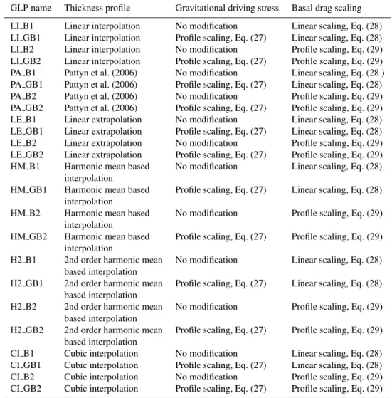
The GLPs are named (Table 1) according to the choice of one of six different thickness interpolation functions (Sect. 3.1) and one of effectively four forcing corrections (Sect. 3.2), giving 24 different GLPs.
To prevent the GLP equations from becoming unwieldy, a scaled dimensionless variable,λ(∈R[0,1]), is used to ex-press distance from theith grid point (i.e. the last grounded grid point) in the x-increasing (i.e. seaward) direction. λis given by
λ=(x−xi)/1x, (5)
wherexis distance in km from the inland edge of the domain (i.e. ice divide),xi is the distance in km of theith grid point
from the inland edge of the domain, and1x is the grid cell size in km. Henceλ=0 at the last grounded grid point and
λ=1 at the first floating grid point. Using this notation, the dimensionless grounding line position is given by
λg=(xg−xi)/1x, (6)
wherexgis the grounding line position in km from the
land-ward edge of the model domain.
The bedrock profileb(λ)is assumed to be linear across the grid cell containing the grounding line,
b(λ)=bi(1−λ)+bi+1λ (7)
though higher resolution bedrock data could be used if avail-able.
3.1 Parameterising the thickness profile
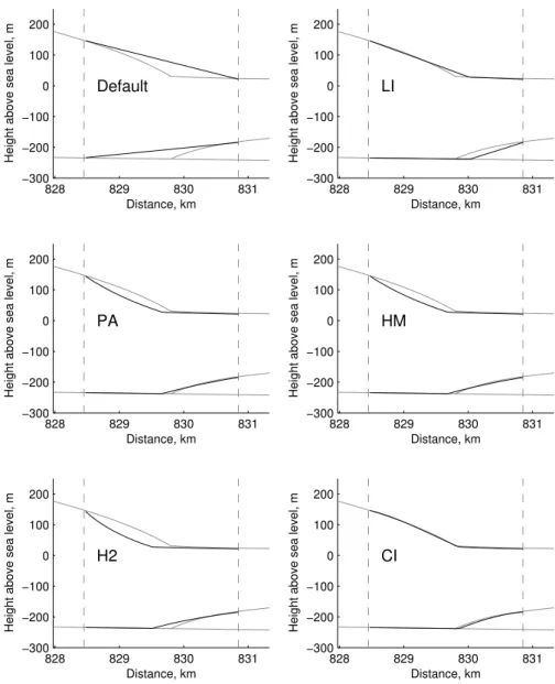
Six methods for constructing a thickness profile across the the grid cell containing the grounding line are presented be-low. These methods are summarised in Table 1 (which also summarises forcing parameterisations), and an example il-lustration of them is shown in Fig. 1. Figure 1 demonstrates how closely these six thickness profiles match a very high resolution thickness profile given the following assumptions: the coarse resolution grid points have thicknesses at the same accuracy as the higher resolution simulation; the grounding line lies at the midpoint of a grid cell. Given that neither of these assumptions are true in general the performance of the different profiles cannot be predicted from Fig. 1. Instead Fig. 1 serves to illustrate the approach, and to emphasize the inaccuracy of the default assumption that the grounding line lies at the last grounded grid point.
The bedrock profile Eq. (7), the thickness profile Eq. (see below), and the flotation condition (Eq. 1) are solved simulta-neously at the grounding line to find grounding line ice thick-ness,Hg, grounding line bedrock depth,bg, and grounding
line position,λg.
3.1.1 Linear interpolation
The simplest reasonable assumption that can be made about the thickness profile across the grid cell containing the grounding line is that of linearity between the known values at grid pointsiandi+1,
H (λ)=Hi(1−λ)+Hi+1λ. (8)
Substituting Eqs. 7 and 8 into 1 atλ=λggives the
ground-ing line position
λg=
ρwbi+ρHi
ρw(bi−bi+1)+ρ(Hi−Hi+1)
. (9)
This parameterisation is abbreviated as LI, see Table 1. 3.1.2 Pattyn’s parameterisation
Instead of making explicit assumptions about both thick-ness and bedrock profiles across the grid cell containing the grounding line, Pattyn et al. (2006) constructed a function of both thickness and bedrock depth,
f=ρwb
Table 1.Summary of grounding line parameterisations (GLPs) used in this study.
GLP name Thickness profile Gravitational driving stress Basal drag scaling
LI B1 Linear interpolation No modification Linear scaling, Eq. (28) LI GB1 Linear interpolation Profile scaling, Eq. (27) Linear scaling, Eq. (28) LI B2 Linear interpolation No modification Profile scaling, Eq. (29) LI GB2 Linear interpolation Profile scaling, Eq. (27) Profile scaling, Eq. (29) PA B1 Pattyn et al. (2006) No modification Linear scaling, Eq. (28 ) PA GB1 Pattyn et al. (2006) Profile scaling, Eq. (27) Linear scaling, Eq. (28) PA B2 Pattyn et al. (2006) No modification Profile scaling, Eq. (29) PA GB2 Pattyn et al. (2006) Profile scaling, Eq. (27) Profile scaling, Eq. (29) LE B1 Linear extrapolation No modification Linear scaling, Eq. (28) LE GB1 Linear extrapolation Profile scaling, Eq. (27) Linear scaling, Eq. (28) LE B2 Linear extrapolation No modification Profile scaling, Eq. (29) LE GB2 Linear extrapolation Profile scaling, Eq. (27) Profile scaling, Eq. (29) HM B1 Harmonic mean based No modification Linear scaling, Eq. (28)
interpolation
HM GB1 Harmonic mean based Profile scaling, Eq. (27) Linear scaling, Eq. (28) interpolation
HM B2 Harmonic mean based No modification Profile scaling, Eq. (29) interpolation
HM GB2 Harmonic mean based Profile scaling, Eq. (27) Profile scaling, Eq. (29) interpolation
H2 B1 2nd order harmonic mean No modification Linear scaling, Eq. (28) based interpolation
H2 GB1 2nd order harmonic mean Profile scaling, Eq. (27) Linear scaling, Eq. (28) based interpolation
H2 B2 2nd order harmonic mean No modification Profile scaling, Eq. (29) based interpolation
H2 GB2 2nd order harmonic mean Profile scaling, Eq. (27) Profile scaling, Eq. (29) based interpolation
CI B1 Cubic interpolation No modification Linear scaling, Eq. (28) CI GB1 Cubic interpolation Profile scaling, Eq. (27) Linear scaling, Eq. (28) CI B2 Cubic interpolation No modification Profile scaling, Eq. (29) CI GB2 Cubic interpolation Profile scaling, Eq. (27) Profile scaling, Eq. (29)
and used interpolation of this function to calculate a ground-ing line position. With the assumption of linear bedrock, this implies a thickness profile of
H (λ)= bi(1−λ)+bi+1λ
bi
Hi(1−λ)+
bi+1
Hi+1λ
. (11)
The grounding line equation, equivalent to Eq. (8) in Pat-tyn et al. (2006), is then
λg=
Hi+1(Hiρ−biρw)
ρw(Hibi+1)−biHi+1.
(12) This parameterisation is abbreviated as PA, see Table 1. 3.1.3 Linear extrapolation
From visual inspection of the thickness profile across the grounding line in very high resolution simulations (e.g. see Fig. 1) the thickness gradient changes abruptly in the vicinity of the grounding line. This and the next (cubic interpolation,
Sect. 3.1.4) choice of thickness profile make use of the gradi-ents landward and seaward of the grounding line in addition to the thicknesses.
Here, linearly extrapolated thickness is used from both the grid points to the landward (i.e. upstream in simulations pre-sented here) of the grounding line,H[up], and to the seaward
(downstream),H[do]:
H[up](λ)=Hi(1+λ)−Hi−1λ (13)
H[do](λ)=Hi+1(2−λ)−Hi+2(1−λ) (14) Substituting Eqs. 7 and 13 into 1, and Eqs. 7 and 14 into 1, atλ=λggives two expressions for grounding line position
λg[up]=
ρHi+ρwbi
ρ(Hi−1−Hi)+ρw(bi−bi+1)
(15)
λg[do]=
ρ(Hi+2−2Hi+1)−ρwbi
ρ(Hi+2−Hi+1)+ρw(bi+1−bi)
(16) where λg[up] and λg[do] are potential grounding line
828 829 830 831 −300
−200 −100 0 100 200
Height above sea level, m
Distance, km
Default
828 829 830 831
−300 −200 −100 0 100 200
Height above sea level, m
Distance, km
LI
828 829 830 831
−300 −200 −100 0 100 200
Height above sea level, m
Distance, km
PA
828 829 830 831
−300 −200 −100 0 100 200
Height above sea level, m
Distance, km
HM
828 829 830 831
−300 −200 −100 0 100 200
Height above sea level, m
Distance, km
H2
828 829 830 831
−300 −200 −100 0 100 200
Height above sea level, m
Distance, km
CI
Fig. 1. Example illustration of the different thickness interpolation functions used in the grounding line parameterisations. The solid grey
lines show the ice sheet profile (bedrock, lower ice surface and upper ice surface from bottom upwards) from a snapshot during the evolution of a very high resolution simulation (1x=0.15 km). The black lines show each of the different thickness profiles (Sect. 3) at lower resolution (1x=2.4 km) for the case where the high resolution simulated grounding line position lies near the centre of the lower resolution grid box. Low resolution grid point positions are shown with vertical grey dashed lines. The LE profile is not shown as it defaults to LI in this case. The default profile corresponds to no parameterisation - the grounding line is assumed to rest at the last grounded grid point.
respectively. Assuming thatH[up]andH[do]intersect in the
grid cell containing the grounding line, the landward and sea-ward thickness equations are combined to give the thickness profile
H (λ)=
H[up](λ) ifλ < λ×
H[do](λ) ifλ≥λ× (17)
whereλ×is the point of intersection of the two extrapolation
functions
λ×= Hi+2−2Hi+1+Hi Hi+2−Hi+1−Hi+Hi−1
(18)
The grounding line position is then given by
λg=
λg[up]ifλg[up],λg[do]≤λ×
λg[do]ifλg[up],λg[do]≥λ× (19)
In the case thatH[up] andH[do] do not intersect in the grid
cell containing the grounding line, no sensible thickness pro-file can be constructed fromH[up]andH[do], and so linear
in-terpolation is used instead (LI, Sect. 3.1.1). LI is also used in the case that two potentially viable grounding line positions are given (i.e.λg[up]≤λ×≤λg[do]). This linear extrapolation
3.1.4 Cubic interpolation
This thickness profile implements higher order interpolation using thicknesses from two grid points landward and two grid points seaward of the grounding line position instead of just one (i.e. grid pointsi−1 andi+2 are used in addition toi
andi+1).
A cubic equation for thickness is fitted across the grid cell containing the grounding line,
H (λ)=aλ3+bλ2+cλ+d, (20)
where four constraints are required to determine the four co-efficients of the cubic,a,b,candd. Two of these are pro-vided by setting the thickness toHi andHi+1at grid points
i and i+1 respectively, as in the other parameterisations. The other two are provided by setting the thickness gradi-ents at i andi+1 to those of the neighbouring grid cells,
(Hi−Hi−1)/1xand(Hi+2−Hi+1)/1x. This gives
a =Hi+2−3Hi+1+3Hi−Hi−1,
b= −Hi+2+4Hi+1−5Hi+2Hi−1,
c=Hi−Hi−1,
d =Hi
Substituting Eqs. 7 and 20 (with the above expressions for the coefficients) into 1 atλ=λggives an expression for the
grounding line position
0=Aλ3g+Bλ2g+Cλg+D, (21)
where
A=Hi+2+3Hi+1−7Hi+3Hi−1,
B = −Hi+2−2Hi+1+5Hi−2Hi−1,
C =Hi−Hi−1+bi
ρw
ρ ,
D=Hi−
ρw
ρ (bi+1+bi).
Note that upper case letters are used for the coefficients sim-ply to emphasize that these are not the same coefficients as in equation 20 above. The cubic equation is solved as in Tuma and Walsh (1998), p7. If no real roots are found, or if more than one root is found within the grid cell containing the grounding line, linear interpolation (LI) is used instead. This parameterisation is abbreviated as CI, see Table 1. 3.1.5 Harmonic mean based parameterisation
The harmonic mean of two numbers a and b is given by 2ab/(a+b). In numerical heat transfer problems a function based on the harmonic mean is used to represent the effect of step changes in conductivity on heat flux at sub-grid scale precision (Patankar, 1980). Here we adopt the approach of Patankar (1980) to construct a thickness profile
H (λ)=
( 1−λ)
Hi
+ λ
Hi+1 −1
. (22)
Substituting Eqs. 7 and 22 into 1 at λ=λg gives an
ex-pression for the grounding line position
0=aλ2g+bλg+c, (23)
where
a= bi+1−bi Hi+1
+bi−bi+1 Hi
,
b= bi Hi+1
−bi+1−2bi Hi
,
c= bi Hi
− ρ
ρw
,
which is solved using the quadratic reduction formula. If no real roots are found, or if more than one root is found within the grid cell containing the grounding line, linear interpola-tion (LI) is used instead. This parameterisainterpola-tion is abbreviated as HM, see Table 1.
3.1.6 Second order harmonic mean based parameterisation
ReplacingHwithH2in Eqs. 22 also gives a tractable thick-ness profile
H (λ)=
v u u
t (1−λ)
Hi2 + λ
Hi2+1
!−1
(24)
Substituting Eqs. 7 and 24 into 1 at λ=λg gives an
ex-pression for the grounding line position
0=aλ3g+bλ2g+cλg+d, (25)
where
a =(Hi−+21−H i−2)(bi2+1+b2i −2bi+1bi),
b=2bi(bi+1−bi)(Hi−+21−Hi−2)+Hi−2(b2i+1+b2i−2bi+1bi),
c=b2i(Hi−+21−Hi−2)+2biHi−2(bi+1−bi),
d =b2iHi−2−ρ2ρw−2.
This cubic equation is solved as in Tuma and Walsh (1998), p7. If no real roots are found, or if more than one root is found within the grid cell containing the grounding line, lin-ear interpolation (LI) is used instead. This parameterisation is abbreviated as H2, see Table 1.
3.2 Parameterising the forcing terms
in the grid box containing the grounding line according to the proportion of the grid box that was grounded. Here we introduce new approaches to modifying both basal drag and gravitational driving stress.
The FGSTSF model used in the current study employs a staggered grid for calculation of velocity. The forcing terms are defined on the staggered grid. This means that the forc-ing terms for the grid cell containforc-ing the groundforc-ing line are defined mid way between theith and (i+1)th grid points, which we will denote by(i+12).
3.2.1 Gravitational driving stress
The gravitational driving stress,G, is given by the right hand side of Eq. 3. For the typical case that bothHandsare linear across the grid box,Gat grid pointi+12 is given by
Gi+1
2=ρg
Hi+Hi+1 2
si+1−si
1x . (26)
For the more general case thatHandsare not linear across the grid box (and note that this is the case even for the linear thickness profile LI due to the discontinuity ins across the grounding line),Gat grid pointi+12can be calculated more accurately by
Gi+1
2=ρg
Z 1
0
H∂s
∂xdλ. (27)
This calculation is carried out numerically by dividing the grid cell containing the grounding line into 1000 equally sized segments and using the approximation of Eq. (26) for each segment. This number was chosen through experimen-tation. Below 100 segments errors due to numerical integra-tion start to become measurable and above 104the computa-tion starts to impact on model run time.
It should be noted that while cumbersome (unwieldy 6th order polynomials are required in places), all the thickness profiles presented in Sect. 3.1 are tractable to analytical so-lutions of the above integral. In practice, a computational implementation of the analytical solution was in some cases found to be highly inaccurate, due to catastrophic cancella-tion.
Note that this modification to the gravitational driving stress forcing term need be carried out only in the grid cell containing the grounding line (so it doesn’t have a measur-able impact on run time).
This profile scaling parameterisation for gravitational driv-ing stress is abbreviated as “G” in Table 1. For example “LI GB1” uses linear interpolation to calculate a thickness profile across the grid cell containing the grounding line, uses the method described above to modify gravitational driving stress in this grid cell, and the linear basal drag correction described below.
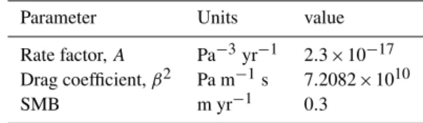
Table 2.Model inputs and parameter values.
Parameter Units value
Rate factor,A Pa−3yr−1 2.3×10⁻¹⁷ Drag coefficient,β2 Pa m−1s 7.2082×10¹⁰
SMB m yr−1 0.3
3.2.2 Basal drag
All the GLPs in the current study involve modification of the basal drag term in the grid cell containing the grounding line, and assume that the basal drag is zero for the floating part of the grid cell.
The simplest parameterisation for basal drag is to scale the basal drag coefficient β2 linearly with the fraction of grounded ice in the grid cell containing the grounding line,
β2
i+12 =β
2(
1−λg) (28)
This linear scaling is referred to as B1, see Table 1.
B1 gives a basal drag force in the grid cell containing the grounding line of−β2ui+1
2(1−λg). Given that the true ve-locity profile in the vicinity of the grounding line is not ex-pected to be linear this scaling is not in general correct. If the velocity profileu(λ)across the grid cell containing the grounding line were known then a more appropriate scaling could be used,
β2
i+12 =β
2 1−
Z λg
0
u(λ)dλ÷
Z 1
0
u(λ)dλ
!
. (29)
Although u(λ) is not known, given that the GLPs pre-sented here all involve prescribing a thickness profile, and that the assumption of linear flux across the grid cell is a safer assumption than that of linear velocity a profile foru(λ)can be calculated,
u(λ)= q(λ)
H (λ), (30)
whereqis the flux given by
q(λ)=qi(1−λ)+qi+1λ. (31)
This profile scaling parameterisation for basal drag (Eqs. 29, 30, and 31) is abbreviated to “B2”, see Table 1. This approach can be taken with both linear (m=1) and non linear (m=1/3) drag laws used in the current study.
4 Experiments
Schoof et al. (2009) experiments 1b and 2b and to Gladstone et al. (2010). The domain size is 2112 km from ice divide (left boundary of domain) to ice front (right boundary of do-main). The grid point spacing,1x, and the timestep, 1t, vary as described below (Sect. 4.1). SMB is prescribed and is spatially and temporally uniform over the domain (except for the first part of the retreat experiments, see below). The rate factorA, drag coefficientβ2, and SMB are given in Ta-ble 2. The bedrock,b, is linear and downsloping with the same gradient as in the MISMIP experiments.
b(x)=511−1.038×10−3x (32)
wherex is the distance from the ice divide, all distances are in metres, andb is measured positively upwards from sea level.
Determination of approach to steady state is by visual in-spection of grounding line evolution plots. The simulation lengths are 35 kyr and 80 kyr for advance and retreat exper-iments (described below) respectively, and this is sufficient for the final grounding line position to be close to steady state in all cases.
As discussed by Gladstone et al. (2010), fixed grid ground-ing line models can exhibit a region containground-ing multiple lo-cally stable grounding line positions, and the limits of this region can be determined by ‘advance’ simulations (in which the grounding line must advance by more than1x as steady state is approached) and “retreat” simulations. This region is a numerical artifact and converges towards zero as res-olution increases (Schoof, 2007a; Gladstone et al., 2010). Both advance and retreat simulations are used in the current study, and their implementation is described in detail in Ap-pendix A.
4.1 Assessing performance
Gladstone et al. (2010) demonstrated that when using the lin-ear thickness GLP (FGSTSF GI in Gladstone et al. (2010), identical to LI B1 in the current study) the steady state grounding line position approaches the analytical solution (Schoof, 2007a) as resolution increases, at least to within a few kilometres, for both advance and retreat simulations.
In the current study convergence of the final (close to steady state) grounding line position with resolution is quan-tified and plotted for performance assessment. Also, two metrics are defined that give a measure of error. The values of these error metrics with increasing resolution are assessed for all GLPs.
The convergence of final grounding line position,xgs, is
assessed by plotting the change in final grounding line posi-tion with increasing resoluposi-tion,1xgs. For a given resolution,
1x, this is given by
1xgs1x= |xgs1x−xgs21x| (33)
where the superscript denotes resolution. 1xgs is plotted
against resolution. This can be done independently for both advance and retreat simulations.
The first of the two error metrics is a quantification of the size of the region of locally stable grounding line positions (Gladstone et al., 2010). This is referred to as “Retreat minus advance” (RMA) and is defined as
RMA=xgr−xga (34)
wherexgr is the final grounding line position from a retreat
experiment andxgais the final grounding line position from
the corresponding advance experiment. It is worth noting thatxgr≥xgafor all simulations in the current study.
The second metric, ACC, is an attempt to measure model accuracy. Accuracy is the discrepancy between simulated and theoretical steady state grounding line positions, but the fact that there are multiple viable modelled steady state grounding line positions (the advance and retreat simulations give different predictions) makes this problematic to quan-tify. Here we have made the choice that our “best” predic-tion for a given model setup is the mid point between the predictions from advance and retreat simulations. Thus ACC is defined by
ACC= |xgr+xga
2 −xgs| (35)
wherexgsis the analytic steady state grounding line position
given by Schoof (2007a). This assumption is not “correct” as a measure of accuracy, but it does give a quantifiable metric that converges to a correct measure of accuracy as the RMA metric approaches zero.
These metrics should not be confused with the “conver-gence” and “accuracy” errors defined by Gladstone et al. (2010).
Since only one steady state solution can exist for the grounding line position in a shelfy-stream model with a lin-ear downsloping bed (Schoof, 2007a), an ideal model solu-tion would have RMA = 0 and ACC = 0.
For each GLP, an advance and retreat simulation is carried out at each resolution, where resolution varies from1x=4.8 km and 1t=0.4 years, to 1x=0.3 km and1t=0.025 years. 1x and1t decrease by a factor of 2 each time giv-ing a total of 5 different resolutions. The GLPs are assessed by comparison of final grounding line position with the ana-lytic solution (Schoof, 2007a), convergence of final ground-ing line position with resolution, and behaviour of the metrics RMA and ACC with increasing resolution.
5 Results
0 10 20 30 40 50 60 70 80 600
800 1000 1200 1400 1600 1800
Grounding line position, km
Time, kyrs ∆ x = 0.3km ∆ x = 4.8km
∆ x = 2.4km ∆ x = 4.8km
∆ x = 0.3km ∆ x = 4.8km
∆ x = 0.3km ∆ x = 4.8km
∆ x = 2.4km ∆ x = 1.2km
Advance, LI_B1 Retreat, LI_B1 Advance, no GLP Retreat, no GLP analytical solution
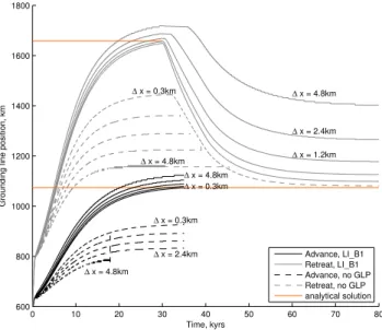
Fig. 2. Time evolution of grounding line position for the LI B1
GLP (solid lines, see Table 1) and for the no-GLP case (dashed lines). Results at the five different resolution levels (from1x= 4.8 km to1x=0.3 km) are shown for both advance (black) and retreat (grey) simulations. The horizontal orange lines indicate the analytical (Schoof, 2007a) steady state grounding line position for the first phase of the retreat simulations (shorter line) and for all other cases (longer line).
grounding line positions and convergence with resolution are compared across GLPs using metrics RMA and ACC.
Several of the thickness parameterisations, specifically LE, CI, HM and H2, are designed to resort to LI in the case that no valid solution can be found. It is worth noting that in practice this happens extremely rarely, and we do not con-sider it significant, except in the case of LE. LE frequently fails to find a valid solution within the grid cell containing the grounding line, and hence frequently reverts to LI. In practice that LE gives results virtually identical to LI.
5.1 Time evolution
The time evolution of the grounding line both for the no-GLP case and for the simplest GLP (LI B1, see Table 1) is shown in Fig. 2. The orange lines indicate the analytical steady state grounding line positions (Schoof, 2007a). The grounding line position in a good advance simulation would be expected to approach the lower orange line at steady state, whereas the grounding line in a good retreat simulation should approach the upper orange line towards the end of the first phase, and the lower line towards the end of the second phase.
In all the advance simulations initially rapid advance grad-ually slows towards steady state (except for the no-GLP
1x=4.8 km simulation, which becomes unstable and fails to complete). In both no-GLP and LI B1 cases the higher resolution final grounding line positions are closer to the
ana-lytic solution than the lower resolution simulations. As found by Gladstone et al. (2010), the no-GLP simulations show er-rors O(100 km) whereas the LI B1 simulations show erer-rors O(10 km) or less (errors are defined here as the difference between final grounding line position and analytic solution). The first phase of the retreat simulations shows behaviour similar to the advance simulations. In the second phase of the retreat simulations, initially rapid retreat gradually slows to-wards steady state, but the onset of retreat is delayed at lower resolutions. This delay can be better understood after consid-ering the finer details of simulated grounding line evolution (see below). Most of the no-GLP simulations become unsta-ble in retreat, with only the1x=0.3 km simulation complet-ing successfully. This numerical instability relates to the in-teraction between basal drag, gravitational driving stress and the grounding line position (Gladstone et al., 2010). The er-rors seen in the LI B1 simulations reduce from O(100 km) to O(10 km) as resolution increases from1x=4.8 km to1x=
0.3 km.
Of the ten no-GLP simulations (both advance and retreat for five different resolutions), the1x=0.3 km retreat sim-ulation is the only one to run to completion with a smaller error (only by O(10 km)) than the equivalent LI B1 simula-tion. Given that most no-GLP simulations either become un-stable and fail to complete or show much greater errors than the equivalent LI B1 simulations, the no-GLP choice is not a viable option and will not be considered further in this study. A close up of grounding line evolution in an advance sim-ulation using the LI B1 GLP is shown in Fig. 3. Although the mean rate of advance is very similar across different res-olutions, the advance appears to occur in steps of size1x
(Fig. 3 upper panel). This behaviour would be expected of simulations without a GLP where the grounding line must always lie at a grid point. A closer inspection (Fig. 3 lower panel) shows that this behaviour is due to sudden accelera-tions of the grounding line as the grounding line passes a grid point, followed by gradual deceleration as the next grid point is approached. This suggests that the LI B1 GLP, whilst al-lowing for grounding line positions anywhere within the grid cell, does not allow for a continuous, smooth response of the grounding line position to the changing state of the system. The ‘state’ of the system is essentially the thickness profile of the whole simulated ice sheet, which determines the grav-itational driving stress and basal drag. In other words, the grounding line resists advance (i.e. advances very slowly) un-til a threshold (corresponding to the grounding line passing a grid point) is passed in the evolving thickness profile, af-ter which very rapid advance occurs. The lower frequency, higher amplitude accelerations seen in the lower resolution simulations indicate that a larger change is needed in the thickness profile to trigger grounding line accelerations.
14.95 15 15.05 15.1 15.15 15.2 970
980 990 1000 1010 1020 1030
Grounding line position, km
Time, kyrs ∆ x = 4.8km
∆ x = 0.3km
12 14 16 18
950 1000 1050
Grounding line position, km
Time, kyrs
∆ x = 0.3km ∆ x = 4.8km
Fig. 3. Close up of the LI B1 advance simulations shown in Fig. 2
showing the step like nature of grounding line advance in detail. Resolutions are 0.3 km, 0.6 km, 1.2 km, 2.4 km and 4.8 km. The horizontal dashed lines in the lower plot indicate grid point loca-tions at1x=4.8 km resolution between 1010 km and 1030 km.
the grid point is approached, but in both retreat and advance simulations the steepest part of the curve occurs immediately after a grid point has been passed.
We suggest that the delayed onset of retreat seen in the second phase of the lower resolution retreat simulations is due to the greater change in thickness profile needed to reach the threshold for the first grounding line retreat acceleration. This is a numerical artifact closely related to the existence of a region of locally stable grounding line positions (Gladstone et al., 2010).
The grounding line evolution over the range of GLPs with resolution fixed at1x=2.4 km is shown in Fig. 5.
Use of the different GLPs does induce a spread in the results, but this spread is smaller than that induced by res-olution for the LI B1 GLP. The time evres-olution and final positions from the advance simulations vary little (within O(10 km) of the analytic solution in all cases), but the retreat varies considerably, by O(102km). The simplest GLP
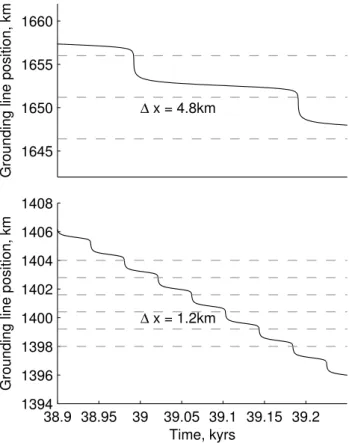
con-38.9 con-38.95 39 39.05 39.1 39.15 39.2 1394
1396 1398 1400 1402 1404 1406 1408
Grounding line position, km
Time, kyrs ∆ x = 1.2km 1645
1650 1655 1660
Grounding line position, km
∆ x = 4.8km
Fig. 4. Close up of the LI B1 retreat simulations shown in
Fig-ure 2. The horizontal dashed lines indicate grid point locations at1x=4.8 km resolution between 1645 km and 1660 km (upper plot) and at1x=1.2 km resolution between 1398 km and 1404 km (lower plot).
ceptually, LI B1, is one of the worst in terms of final ground-ing line position from the retreat simulation. The best GLP by this measure is H2 GB2.
0 20 40 60 80 400
600 800 1000 1200 1400 1600 1800
Grounding line position, km
Time, kyrs H2_GB2
LI_B1
Advance Retreat
Fig. 5. Time evolution of grounding line position for all GLPs
at a resolution of 2.4 km. The final grounding line positions from the advance simulations have been extended with dashed lines to facilitate comparison against the retreat simulations. The retreat simulations for the simplest (LI B1) and “best” (H2 GB2) GLPs are shown with dashed lines.
1554 1556 1558
Grounding line position, km
37.22 37.24 37.26 37.28 37.3 37.32 37.34 1452 1454 1456
LI_B1 H2_GB2
37.22 37.24 37.26 37.28 37.3 37.32 37.34 −1
−0.5 0
Grounding line velocity, km/yr
Time, kyrs LI_B1 H2_GB2
Fig. 6. Close up of retreat simulations for the simplest (LI B1)
and “best” (H2 GB2) GLPs run at 2.4 km resolution. The top panel shows grounding line position with time (the y-axes are offset but with identical scaling to facilitate comparison) and the lower panel shows grounding line velocity with time (i.e. velocity of the ground-ing line itself, not the velocity of the ice at the groundground-ing line).
101 102
RMA metric, km
RMA ∝∆ x RMA ∝∆ x2
4.8 2.4 1.2 0.6 0.3
101 102
ACC metric, km
Resolution (i.e. ∆ x), km ACC ∝∆ x
ACC ∝∆ x2
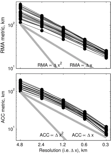
Fig. 7. Error metrics ACC and RMA (Sect. 4.1) against resolution.
Results are shown for all GLPs (see Table 1). Example first order and second order convergence (grey bars) are shown for comparison (note that the starting point of the grey bars is arbitrary, it is the gradient that defines the order of convergence).
5.2 Steady state grounding line position
The error metrics are plotted against grid resolution for all GLPs in Fig. 7. Both metrics (ACC and RMA, described in Sect. 4.1) decay as resolution increases, typically linearly or slightly slower (by comparison to grey bars in Fig. 7). Con-vergence of the final grounding line position approaches first order as resolution increases (Fig. 8).
2.4 1.2 0.6 0.3 100
101 102
Resolution (i.e. ∆ x), km
Convergence (i.e.
∆
x gs
), km
∆ xgs∝∆ x ∆ xgs∝∆ x2
Advance Retreat
Fig. 8. Convergence of steady state grounding line position
(de-scribed in Sect. 4.1).1xgsis plotted against resolution for all GLPs
(see Table 1). Example first order and second order convergence (grey bars) are shown for comparison.
RMA is a more reliable measure of convergence than ACC as it is purely a measure of internal consistency.
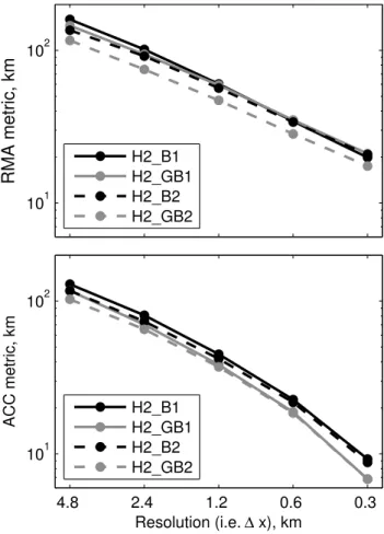
Figure 9 shows how the different forcing term corrections (B1, B2 and G, Sect. 3.2) impact on performance for a spe-cific thickness interpolation (in this case H2, Sect. 3.1.6). Al-though the more sophisticated handling (i.e. H2 GB2) does show smaller errors according to both metrics, the impact is small, and RMA and ACC appear to converge at similar rates for the different forcing term corrections. This result is sim-ilar for other thickness interpolations (not shown), with the GB2 corrections generally giving the smallest errors and the B1 correction giving the largest errors. The differences are not large and convergence of RMA and ACC does not vary greatly.
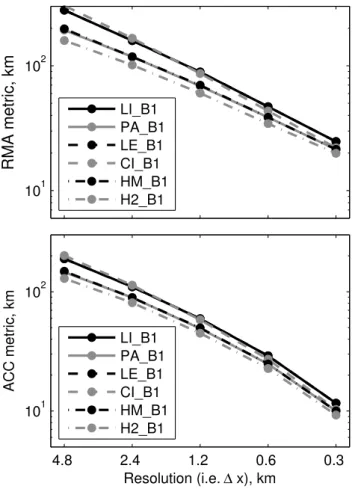
Figure 10 shows convergence of RMA and ACC for the different thickness interpolations (Sect. 3.1) when the sim-plest basal drag correction (B1, Sect. 3.2.2) is used. The lin-ear interpolation, LI, shows the greatest error (except at the lower resolutions where CI is worse) and the second order harmonic mean based interpolation, H2, shows the lowest error. The cubic interpolation GLP, CI, appears to converge slightly faster than the others.
The “best” GLP is H2 GB2. This gives the lowest errors at all resolutions and for both error metrics. The previously published LI B1 (Gladstone et al., 2010) gives poor perfor-mance. PA B1, based on the parameterisation of Pattyn et al. (2006), gives mid range performance.
101 102
RMA metric, km
H2_B1 H2_GB1 H2_B2 H2_GB2
4.8 2.4 1.2 0.6 0.3
101 102
ACC metric, km
Resolution (i.e. ∆ x), km H2_B1
H2_GB1 H2_B2 H2_GB2
Fig. 9. Error metrics ACC and RMA (Sect. 4.1) plotted against
resolution for the GLPs using the 2nd order harmonic mean based thickness profile (H2, Sect. 3.1.6). Results are shown for all forcing term corrections (see Table 1).
5.3 Non-linear drag law
101 102
RMA metric, km
LI_B1 PA_B1 LE_B1 CI_B1 HM_B1 H2_B1
4.8 2.4 1.2 0.6 0.3
101 102
ACC metric, km
Resolution (i.e. ∆ x), km LI_B1
PA_B1 LE_B1 CI_B1 HM_B1 H2_B1
Fig. 10. Error metrics ACC and RMA (Sect. 4.1) plotted against
resolution for the GLPs using the simplest forcing term correc-tion, B1 (Sect. 3.2.2). Results are shown for all thickness profiles (Sect. 3.1).
6 Discussion
The aim of the current study is to provide an easily imple-mentable and computationally efficient approach to param-eterising the grounding line that can reduce grounding line errors in full ice sheet models, and to justify this approach through experimentation. The GLPs presented in the current study could all be extended to two horizontal dimensions, though this might not be trivial in the case of the more so-phisticated parameterisations.
It is clear that the difference between not using a GLP and using the simplest GLP (namely LI B1) is large (Sect. 5.1, see also Gladstone et al. (2010)). Given the large errors and the unstable nature of grounding line retreat in a fixed grid shelfy-stream model without a GLP, use of a GLP is neces-sary, though which of the present GLPs to use is less clear.
In Sect. 5.2 the more sophisticated GLPs were shown to give better performance than the simpler ones, but this per-formance difference is not as large as the difference between no GLP and the simplest GLP. The best GLP in the current
100 101
RMA metric, km
RMA ∝∆ x
RMA ∝∆ x2
4.8 2.4 1.2 0.6 0.3
100 101
ACC metric, km
Resolution (i.e. ∆ x), km ACC ∝∆ x
ACC ∝∆ x2
Fig. 11. Error metrics ACC and RMA (Sect. 4.1) against resolution
when using the non-linear drag law (Sect. 5.3). Results are shown for all GLPs (see Table 1). Example first order and second order convergence (grey bars) are shown for comparison.
study, H2 GB2 (Sect. 3.1.6), gives errors comparable to the worst GLP, LI B1, run at twice as fine a resolution (i.e. dou-ble the number of grid points). This result holds for both the linear and non-linear drag laws. When implemented in an ice sheet model with two horizontal dimensions, use of H2 GB2 instead of LI B1 would represent a significant (at least factor 8) saving in computational resource. However, LI B1 would be easier to implement than H2 GB2 in two horizontal di-mensions. Although errors at a given resolution are reduced in more sophisticated GLPs, the rate of convergence does not vary significantly across GLPs. None of the GLPs presented here can fully overcome the grounding line problem inher-ent to fixed grid models (Vieli and Payne, 2005): very high resolution is still needed.
GLPs. However, this is not the case, due to the quality of fit of the CI interpolation varying during model evolution. This suggests that the approach of choosing one interpola-tion funcinterpola-tion for thickness over the the grid cell containing the grounding line is fundamentally limited, and that such a function would itself need to evolve as the model evolves.
Another way of viewing this problem is in terms of the step like behaviour in grounding line evolution (Sect. 5.1). The GLPs are intended to solve the grounding line problem by allowing the grounding line to move smoothly across the grid cells. But grounding line movement still exhibits rapid accelerations as grid points are passed, demonstrating that the grounding line problem is only partially solved using the approaches in the current study.
This behaviour is not surprising - there is no a priori rea-son why the thickness profile over the grid cell containing the grounding line should match one particular interpolation function. However, the default assumption that the ground-ing line always lies at the last grounded grid point is clearly incorrect. The capacity of the GLPs presented here to allow the grounding line to lie at any point within a grid cell is not only a conceptual improvement, but gives demonstrably better results then the default assumption.
A more accurate method of parameterising the grounding line would therefore need to use a function that evolves as the model state evolves, possibly parameterised based on de-tailed studies of high resolution simulations. However, given that mesh adaptivity gives a true representation of the under-lying equations and has been shown to address the ground-ing line problem well (Gladstone et al., 2010; Durand et al., 2009) adaptivity may provide a better solution than very complicated parameterisations.
An alternative approach to parameterising the grounding line was implemented by Pollard and DeConto (2009). Two separate models for grounded and floating ice were con-nected across the grounding line using an ice flux bound-ary condition. Cross grounding line ice flux was calculated as a function of ice thickness, rate factor, basal drag, and a scaling factor to represent buttressing (Eq. 29 in Schoof (2007a), see also Schoof, 2007b). This specification of flux is valid in the special case of a flow-line model for plug flow where “ice is not too cold, sliding is slow, or the ice sheet is wide” (Schoof, 2007a). Errors associated with this flux prescription method in the case of actual ice streams and ice shelves have not yet been quantified, though the assumptions are more likely to be invalid away from steady state (Schoof, 2007b). A comparison against the GLPs described in the cur-rent study, and against very high resolution simulations (pos-sibly using adaptivity) in a real world context would form a useful further study.
The flux prescription approach described above does not address the restriction imposed by fixed grid grounding line models that the grounding line must advance or retreat in steps of one grid cell at a time (which in turn causes step changes in the basal drag). The solution of Pollard and
De-Conto (2009) to this limitation was to apply the prescribed flux either at the grounding line or downstream of it, depend-ing on a flux criterion (details in supportdepend-ing materal, Pollard and DeConto (2009)). The criterion overcomes the inconsis-tency between advance and retreat simulations but is without rigourous physical justification.
7 Conclusions
A general approach to parameterising the grounding line in fixed grid ice sheet models has been presented, expanding on previous work (Pattyn et al., 2006; Gladstone et al., 2010). The approach, centred on interpolating ice thickness over the grid cell containing the grounding line, shows greater relia-bility and an order of magnitude improvement in simulated grounding line position compared to the default assumption that the grounding line lies at the last grounded grid point.
Twenty four grounding line parameterisations (GLPs) have been presented, and tested in a fixed grid shelfy-stream model. The performance difference between the best and worst is comparable to a doubling of resolution. The GLPs are amenable to adaptation to two horizontal dimensions, where a doubling of resolution has a large (at least factor 8) impact on computational resource.
Two of the GLPs have been previously published. The simplest GLP, LI B1 (Gladstone et al., 2010), gives poor per-formance compared to the other GLPs. PA B1, based on the work of Pattyn et al. (2006), gives mid range performance. The new parameterisation H2 GB2, which includes a correc-tion to the gravitacorrec-tional driving stress, gives the best perfor-mance.
None of these GLPs fully solve the grounding line prob-lem, very high resolution is still needed. This is consis-tent with the conclusion of Schoof (2007a) that adaptivity (or high resolution) near the grounding line is essential. A combination of adaptive mesh refinement and a GLP would provide the most computationally efficient approach to min-imising grounding line errors.
Appendix A
Advance and retreat simulations
Simulations are carried out in pairs: an advance simulation in which the steady state grounding line position is approached from landward, and a retreat simulation in which the steady state grounding line position is approached from seaward.
Both retreat and advance simulations are initialised from a uniform slab of ice 200 m thick. Advance simulations are simply spun up for 35 kyr using a constant forcing. The final grounding line position is close to steady state.
The retreat simulations have two phases. In the first phase advance occurs and in the second phase retreat occurs. The first phase of a retreat simulation has enhanced forcing under which the grounding line will advance much further than in the corresponding advance simulation. The second phase has forcing identical to that of the corresponding advance simu-lation as steady state is approached in retreat. As with the ad-vance simulations, the final grounding line position is close to steady state.
The details of the forcing modification for retreat exper-iments are now described. During the first phase of 30 kyr the SMB and rate factor are both modified, and these are re-turned linearly to their standard values over the first 10 kyr years of the second phase. A further 40 kyr with forcing con-stant and identical to the corresponding advance simulation are then run in order to reach the final steady state, giving a total run length of 80 kyr for the retreat simulations.
It is not strictly necessary to approach steady state in the first phase of the retreat simulations, so long as significant retreat occurs in the second phase, to fulfil the requirement that the final grounding line position in a retreat simulation is approached from seaward.
The rate factor is given by
AR(t∗)=
A
10 t
∗<0
A
10(1−t
∗/104)+At∗/1040≤t∗≤104
A t∗≥104
(A1)
whereARis the (time varying) rate factor for the retreat
sim-ulation, andt∗is the time in years (measured positively for-ward in time) from the start of the second phase of the sim-ulation (i.e.t∗=t−35 kyr wheret is the time in years from the start of the simulation). The SMB is given by
aR(t∗)=
a+0.4 t∗<0
a+0.4(1−t∗/104)0≤t∗≤104
a t∗≥104,
(A2)
whereaRis the (time varying) SMB for the retreat
simula-tion anda is the SMB used in the corresponding advance simulation, both measured in m yr−1
Note that the forcing in both advance and retreat experi-ments is identical (i.e.AR=AandaR=a) and constant as
the final grounding line position is approached.
Acknowledgements. The authors would like to thank Steve Price
and Frank Pattyn for their constructive reviews which led to improvements in the clarity of the manuscript. This work was supported by the UK’s National Centre for Earth Observation cryosphere and climate themes, the NERC Joint Weather and Climate Research Programme, and the project “Understanding contemporary change in the West Antarctic ice sheet” funded by NERC standard grants NE/E006256/1 and NE/E006108/1.
Edited by: G. H. Gudmundsson
References
Durand, G., Gagliardini, O., de Fleurian, B., Zwinger, T., and Le Meur, E.: Marine ice sheet dynamics: Hystere-sis and neutral equilibrium, J. Geophys. Res.-Earth, 114, doi:10.1029/2008JF001170, 2009.
Gladstone, R., Lee, V., Vieli, A., and Payne, A.: Grounding Line Migration in an Adaptive Mesh Ice Sheet Model, J. Geophys. Res.-Earth, 115, doi:10.1029/2009JF001615, 2010.
Goldberg, D., Holland, D. M., and Schoof, C.: Grounding line movement and ice shelf buttressing in marine ice sheets, J. Geo-phys. Res.-Earth, 114, doi:10.1029/2008JF001227, 2009. Katz, R. F. and Worster, M. G.: Stability of ice-sheet
ground-ing lines, P. Roy. Soc. A.-Math. Phy., 466, 1597–1620, doi:10.1098/rspa.2009.0434, 2010.
Mercer, J.: West Antarctic Ice Sheet and CO2Greenhouse Effect – Threat of Disaster, Nature, 271, 321–325, 1978.
Patankar, S.: Numerical Heat Transfer and Fluid Flow, Taylor & Francis, 1980.
Pattyn, F., Huyghe, A., De Brabander, S., and De Smedt, B.: Role of transition zones in marine ice sheet dynamics, J. Geophys. Res.-Earth, 111, doi:10.1029/2005JF000394, 2006.
Pollard, D. and DeConto, R. M.: Modelling West Antarctic ice sheet growth and collapse through the past five million years, Nature, 458, 329–332, doi:10.1038/nature07809, 2009.
Schoof, C.: Ice sheet grounding line dynamics: Steady states, stability, and hysteresis, J. Geophys. Res.-Earth, 112, doi:10.1029/2006JF000664, 2007a.
Schoof, C.: Marine ice-sheet dynamics. Part 1. The case of rapid sliding, J. Fluid Mech., 573, 27–55, doi:10.1017/S0022112006003570, 2007b.
Schoof, C., Pattyn, F., and Hindmarsh, R.: MISMIP: Marine Ice Sheet Model Intercomparison Project, http://homepages.ulb.ac. be/∼fpattyn/mismip/, 2009.
Tuma, J. and Walsh, R.: Engineering Mathematics Handbook, Mc-Graw Hill, 1998.