Geosci. Model Dev., 6, 353–372, 2013 www.geosci-model-dev.net/6/353/2013/ doi:10.5194/gmd-6-353-2013
© Author(s) 2013. CC Attribution 3.0 License.
Geoscientiic
Model Development
Open Access
Geoscientiic
Air quality modelling using the Met Office Unified Model
(AQUM OS24-26): model description and initial evaluation
N. H. Savage, P. Agnew, L. S. Davis, C. Ord´o ˜nez, R. Thorpe, C. E. Johnson, F. M. O’Connor, and M. Dalvi
Met Office, Fitzroy Road, Exeter, EX1 3PB, UK
Correspondence to:N. H. Savage ([email protected])
Received: 24 August 2012 – Published in Geosci. Model Dev. Discuss.: 10 October 2012 Revised: 6 February 2013 – Accepted: 19 February 2013 – Published: 12 March 2013
Abstract.The on-line air quality model AQUM (Air Quality in the Unified Model) is a limited-area forecast configuration of the Met Office Unified Model which uses the UKCA (UK Chemistry and Aerosols) sub-model. AQUM has been devel-oped with two aims: as an operational system to deliver re-gional air quality forecasts and as a modelling system to con-duct air quality studies to inform policy decisions on emis-sions controls. This paper presents a description of the model and the methods used to evaluate the performance of the fore-cast system against the automated UK surface network of air quality monitors. Results are presented of evaluation studies conducted for a year-long period of operational forecast tri-als and several past cases of poor air quality episodes. The results demonstrate that AQUM tends to over-predict ozone (∼8 µg m−3mean bias for the year-long forecast), but has a
good level of responsiveness to elevated ozone episode con-ditions – a characteristic which is essential for forecasting poor air quality episodes. AQUM is shown to have a nega-tive bias for PM10, while for PM2.5the negative bias is much
smaller in magnitude. An analysis of speciated PM2.5 data
during an episode of elevated particulate matter (PM) sug-gests that the PM bias occurs mainly in the coarse compo-nent. The sensitivity of model predictions to lateral boundary conditions (LBCs) has been assessed by using LBCs from two different global reanalyses and by comparing the stan-dard, single-nested configuration with a configuration having an intermediate European nest. We conclude that, even with a much larger regional domain, the LBCs remain an impor-tant source of model error for relatively long-lived polluimpor-tants such as ozone. To place the model performance in context we compare AQUM ozone forecasts with those of another forecasting system, the MACC (Monitoring Atmospheric
Composition and Climate) ensemble, for a 5-month period. An analysis of the variation of model skill with forecast lead time is presented and the insights this provides to the relative sources of error in air quality modelling are discussed.
1 Introduction
direct aerosol effects due to radiation scattering and indirect effects such as the nucleation of cloud droplets by partic-ulates. A new collaborative project – COST-ES1004 – has been initiated with the objective of clarifying and quantify-ing the improvements to meteorological forecasts by includ-ing on-line composition modellinclud-ing.
The UK Met Office Unified Model (MetUM) is a weather and climate modelling system which is used across a very wide range of spatial and temporal scales, from short-range weather forecasting at 1.5 km resolution (Price et al., 2011) to multi-decadal simulations in an Earth system model con-figuration (Collins et al., 2011). We have developed a config-uration of the MetUM for use as an on-line regional air qual-ity model – AQUM (Air Qualqual-ity in the Unified Model). This model builds on the work of the United Kingdom Chemistry and Aerosols (UKCA) project (Morgenstern et al., 2009; O’Connor et al., 2013), which has constructed a new frame-work for atmospheric composition modelling within the Me-tUM. The type of parameterisations used in UKCA and the level of complexity in representing the Earth system can be selected as appropriate to the problem under investigation. AQUM has been developed to fulfil two purposes: (i) the op-erational delivery of daily air quality forecasts and (ii) to en-able atmospheric modelling studies to address scientific and air quality policy-related questions. We have chosen to de-velop a chemistry and aerosol model online in the MetUM so that the feedbacks of atmospheric composition on meteo-rology can, in due course, be included in the weather forecast model. However, this application is not examined in this pa-per, which focuses exclusively on air quality modelling.
In Sect. 2 of this paper we present an overview of the AQUM modelling system. We then describe the verification methodology we have used to evaluate the model in Sect. 3. In Sect. 4 we present a summary of the evaluation studies we have carried out on both operational forecasts and particular past air quality episodes, comparing model predictions with a surface observation network. A summary of the results is presented in Sect. 5 and a short description of the model de-velopments planned for AQUM is given.
2 Model description
2.1 Physical model overview
AQUM is currently operated with a 12-km horizontal reso-lution grid covering much of Western Europe (see Fig. 9). The native model grid is on a rotated-pole coordinate sys-tem with the North Pole at latitude 37.5◦
and longitude at 177.5◦
. There are 38 vertical levels up to a model top height of 39 km. This would be considered high for an off-line air quality model, but for on-line modelling a height of this or-der is necessary for accurate modelling of the meteorologi-cal system. The resolution and domain were selected to en-able regional-scale ozone and particulate matter (PM) events
impacting the United Kingdom to be modelled. The model physics configuration is based on the Met Office’s North At-lantic and European Model (NAE). A description of this con-figuration is given in Bush et al. (2006), although some fur-ther minor developments were made to the model prior to it forming the basis of the AQUM model described here.
The MetUM dynamical core is non-hydrostatic and fully compressible, and no shallow atmosphere approximations are made. Semi-implicit, semi-Lagrangian time integration methods are used and a positive definite semi-Lagrangian tracer advection scheme is used to advect aerosols and gases (Davies et al., 2005). Boundary layer mixing (including that of aerosols and gases) is parameterised with a non-local, first order closure, multi-regime scheme (Lock et al., 2000). Convection is represented with a mass flux scheme with downdraughts, momentum transport and CAPE (convective available potential energy) closure (Gregory and Rowntree, 1990). The land surface scheme, MOSES II, is a nine tile, flux-blended surface exchange approach and includes an ur-ban tile (Essery et al., 2003). The model uses the Edwards– Slingo flexible multi-band two-stream code for long- and short-wave radiation with 6 SW and 9 LW bands (Edwards and Slingo, 1996). Wilson and Ballard (1999) microphysics is employed and extended to include prognostic ice and snow, rain and graupel. The model uses the diagnostic cloud scheme described by Smith (1990).
2.2 Gas phase chemistry scheme
The AQUM gas phase chemistry is a further development of the UKCA tropospheric chemistry scheme (O’Connor et al., 2013), but with a new chemical mechanism added specif-ically for regional air quality (RAQ) modelling. This RAQ mechanism includes 40 transported species (16 of them emit-ted), 18 non-advected species, 116 gas phase reactions and 23 photolysis reactions (see Supplement, Tables S1–S5). Re-moval by wet and dry deposition is considered for 19 and 16 species respectively (see Tables S1 and S6 in the Supple-ment). Unlike the standard tropospheric chemistry described in O’Connor et al. (2013), this scheme includes the oxida-tion of both C2–C3 alkenes (ethene and propene), isoprene and aromatic compounds such as toluene and o-xylene, as well as the formation of organic nitrate. It is adapted from the mechanism presented in Collins et al. (1997) with the ad-ditional reactions described in Collins et al. (1999) and some further modifications (in particular to the isoprene and aro-matic chemistry mechanisms). For more details on the RAQ chemistry scheme refer to the Supplement. Note that sulphur chemistry is not currently included in the RAQ mechanism, but is treated in the aerosol scheme (see Sect. 2.3). The con-centrations are updated using a backward Euler solver with a time step of 75 s in the studies described in this paper.
Sanderson et al., 2007) with surface resistance terms calcu-lated for each tile. The aerodynamic and quasi-laminar resis-tance are calculated based on the roughness length, canopy height and surface heat flux. Wet deposition is parameterised as a first order loss rate, calculated as a function of the model’s three-dimensional convective and large-scale precip-itation in a manner adapted from Giannakopoulos (1998) and Giannakopoulos et al. (1999). Photolysis rates are calculated with the on-line photolysis scheme Fast-J (Wild et al., 2000), which is coupled to the modelled liquid water and ice con-tent, and sulphate aerosols on a time step basis.
2.3 Aerosol scheme
The current AQUM configuration uses the Coupled Large-scale Aerosol Simulator for Studies in Climate (CLASSIC) aerosol module. A short description will be given here – for further details see Appendix A of Bellouin et al. (2011) and references therein.
The scheme contains six prognostic tropospheric aerosol types: ammonium sulphate, mineral dust, fossil fuel black carbon (FFBC), fossil fuel organic carbon (FFOC), biomass burning aerosols and ammonium nitrate. In addition, there is a diagnostic aerosol scheme for sea salt and a fixed clima-tology of biogenic secondary organic aerosols (BSOA) from the oxidation of terpenes from vegetation. It is a bulk aerosol scheme, where the aerosol species are treated as an external mixture and the mass of each aerosol type is the prognos-tic variable. Each aerosol type is assumed to have a fixed log-normal size distribution (apart from dust, which is repre-sented with six size bins). For information on the median ra-dius, geometric standard deviation, density and optical prop-erties see Bellouin et al. (2011).
The model has two-way coupling of oxidants between the aerosol and gas phase chemistry schemes. Thus, emissions of sulphur dioxide (SO2)and dimethyl sulphide (DMS) are
oxidised into sulphate aerosol (SO24−) by oxidants whose concentrations are calculated in the RAQ chemistry scheme, and the depleted oxidant fields are then passed back to the RAQ scheme to ensure consistency. Sulphate aerosol is rep-resented by Aitken and accumulation modes and an addi-tional tracer for sulphate dissolved in cloud droplets. Sul-phate mass is assumed to all be in the form of ammonium sulphate [(NH4)2SO4]. Emissions of DMS from oceans are
parameterised as function of wind speed based on the ap-proach of Wanninkhof (1992), with sea water concentrations from a 1◦×1◦climatology (Kettle et al., 1999).
Ammonia (NH3)is a transported tracer in the model and
is removed from the atmosphere by the formation of ammo-nium sulphate (as well as by dry and wet deposition); any ex-cess ammonia can react with nitric acid (HNO3)to form
am-monium nitrate aerosol (NH4NO3). Thermal decomposition
of ammonium nitrate to nitric acid and ammonia is permitted according to the equilibrium model described by Ackermann et al. (1995). Nitric acid concentrations are derived from the
RAQ scheme and depleted by nitrate aerosol formation. The mass of nitrate aerosol formed goes into an accumulation mode and cloud formation transforms some of the accumu-lation mode into the dissolved mode, as with sulphate.
The mineral dust scheme has six size bins covering radii from 0.0316 µm to 3.16 µm. The emissions fluxes depend on vegetation fraction, soil roughness length and moisture, and near-surface wind speeds. The dust in these six bins is trans-ported and deposited by gravitational settling, turbulence and below-cloud scavenging.
FFBC, FFOC and biomass burning aerosols have three modes – fresh, aged and in-cloud. Ageing is represented as an exponential decay. Sea salt is represented in a diagnos-tic manner with number concentrations over the open ocean calculated as a function of the wind speed at a height of 10 m (O’Dowd et al., 1999). Biogenic secondary organic aerosols from the oxidation of terpenes are included as a three-dimensional monthly mean climatology at 5◦
×5◦ res-olution (Derwent et al., 2003).
The direct radiative effects of all aerosols are included in the model by use of wavelength dependent scattering and absorption coefficients calculated off-line according to Mie theory. The off-line calculations include the effects of hy-groscopic growth for the sulphate, sea salt, nitrate, biomass burning, FFOC and biogenic aerosols with each aerosol type assumed to have a fixed size distribution and optical proper-ties. All aerosol species except mineral dust and FFBC are considered to act as cloud condensation nuclei. The param-eterisations of the first and second indirect effects are as de-scribed by Jones et al. (2001). Although aerosol couplings to meteorological processes are included in our model configu-ration, the impact of this on meteorology is not addressed in this paper, but will be examined in a subsequent publication.
2.4 Lateral boundary conditions
Lateral boundary conditions use the method of Davies (1976), which involves relaxing the interior flow near the boundaries towards the externally prescribed flow. Relaxation involves blending of the LBCs and the limited-area model (LAM) over several grid points. For further details see Davies (2013).
configuration, and benefits from the data assimilation carried out by the GEMS and MACC projects. A reanalysis prepared as part of the GEMS project was used to provide chemical LBCs for the case studies we have conducted, whilst real time MACC global model fields are used for the AQUM operational forecasts. The sensitivity of AQUM forecasts to chemical LBCs is discussed further in Sect. 4.3.
2.5 Model initialisation and run cycle
For the period of the model evaluations described in Sect. 4, the operational forecast model ran once per day out to 48 h ahead (although the system has since been upgraded and now provides forecasts out to 5 days ahead). The initial conditions for chemistry and aerosol species for a new AQUM forecast run are taken from theT+24 forecast of the previous model run. No independent data assimilation cycle was used in the forecasts. However, the initial conditions for the meteorol-ogy used Met Office analyses from the NAE model and so inherit assimilated fields for meteorological parameters pro-duced using 4-D-variational assimilation. There is no data assimilation of chemical species either directly or indirectly, although the chemical LBCs from the GEMS/MACC global model benefit from the data assimilation within those mod-els.
2.6 Emissions
The anthropogenic pollutant emissions used in AQUM are derived from three datasets. The highest resolution emissions data are from the UK National Atmospheric Emissions In-ventory (NAEI, MacCarthy et al., 2011), which has a 1-km resolution and covers the UK only. Outside of the UK, emis-sions are taken from the European Monitoring and Evalu-ation Programme (EMEP) emissions datasets, which cover Europe at 50-km resolution (Mareckova et al., 2010, and sim-ilar reports for previous years). These EMEP emission fields are not further down-scaled with surrogates (such as popula-tion density), but are taken as they are. Finally, a 5-km reso-lution gridded shipping emissions dataset produced by Entec UK Ltd on behalf of Defra (Whall et al., 2010) is used to rep-resent emissions for waters around the UK. Where they over-lap, shipping data from Entec replaces data from the NAEI and EMEP SNAP sector 8 (“other mobile sources and ma-chinery”) in the NOS (“North Sea”) and ATL (“remaining North-East Atlantic region”) regions. This process ensures there is no duplication of shipping emissions. The Entec dataset was only compiled for 2007, so for other years these data are scaled according to published totals from EMEP. Data from all three sources are interpolated to the AQUM 12 km grid prior to merging. The main benefits of the process we have adopted of merging data from 3 different sources are (i) the NAEI and EMEP data are updated on an annual basis; (ii) we ensure that the highest resolution datasets available for the UK are used. The use of a lower resolution dataset
over Europe is not a serious limitation: numerical diffusion on the 12-km AQUM grid inherently disperses the emissions at source, and by the time any emissions from Europe reach the UK they have generally diffused in the atmosphere to an extent such that any detailed “memory” of the source spatial distribution has been lost.
Six key families of pollutants are provided in the emis-sions datasets described above: carbon monoxide (CO), sul-phur oxide gases (SOx), volatile organic compounds (VOCs),
nitrogen oxides (NOx=NO2+NO), fine particulate matter
with a diameter of 2.5 µm or less (PM2.5), PM coarse with
a diameter from 2.5 to 10 µm (defined as PM10–PM2.5)and
NH3. For use in AQUM the non-methane VOC component
of emissions is partitioned into the species required by the RAQ chemical mechanism: formaldehyde, ethene, propene, isoprene, o-xylene, toluene, acetaldehyde, ethane, propane, butane, acetone and methanol (see Table S1 in the Supple-ment). The inventory total VOC emitted mass is apportioned amongst these species according to the tabulated data for 2006 given by Dore et al. (2008), in a manner which en-sures the total VOC mass is accounted for. This same report provides further information that we have used to provide a separate traffic-specific speciation of emitted VOC over the UK.
For gas phase emissions AQUM currently has a simple treatment of the vertical emission profile: all emissions are spread equally over the first four model levels (20, 80, 180 and 320 m). This profile was selected on the basis of sensi-tivity tests under ozone episode conditions. Clearly this is a significant oversimplification, but a more sophisticated treat-ment is currently being developed (see Sect. 5). However, in practice the representation of a physically realistic pro-file is limited in an Eulerian model by the spacing of model grid levels and numerical diffusion. Factors representing the monthly, daily and hourly temporal variations are applied to anthropogenic gas phase emissions. The hourly variations, derived from an analysis of traffic cycles, are applied to all species.
The CLASSIC aerosol scheme used by AQUM requires emissions of specific aerosol and gas phase species: FFOC, FFBC, biomass burning aerosol, DMS and sulphur (S) in SO2for sulphate production, NOx and ammonia for nitrate
aerosol production, mineral dust and sea salt. The last two species have on-line source terms which depend on meteorol-ogy and surface properties. Nitrate aerosol can be regarded as being formed entirely from gas phase precursors (secondary aerosol). Sulphate aerosol is largely secondary, but also con-tains a small primary component. We currently model the latter by emitting an equivalent amount of gas phase SO2
which is then oxidised to sulphate within CLASSIC. The UK anthropogenic emissions of SOxrequired by CLASSIC are
split into high- (320 m) and low-level (surface) components, representing emissions from chimneys and surface sources, respectively. Volcanic SOx emissions are derived from the
Other gas phase emissions for secondary aerosol production are accounted for by the emissions derived from the three in-ventories described above. However, emissions are required for primary particulate matter. The emissions datasets gen-erated by EMEP, NAEI and ENTEC provide only total PM; thus, in order to use these high-resolution emissions datasets, we must apportion the total PM amongst the different pri-mary species required by CLASSIC. In order to achieve this we have used a dataset compiled by TNO for the GEMS project (Visschedijk et al., 2007). This dataset provides an es-timate of the percentage contribution of key aerosol species to the total PM in each SNAP sector. The largest contribution in all sectors of the TNO speciation is “other primary emis-sions”, i.e. non specific PM. Some definite choice must be made about how to apportion this mass amongst the CLAS-SIC species. We have apportioned both “fine” and “coarse other” primary PM10to FFBC in the CLASSIC scheme. This
choice is somewhat arbitrary and is simply a device to en-able all emitted PM to be accounted for. The vertical dis-tribution of aerosol sources are split into high (320 m) and surface sources of sulphate, black carbon and organic carbon fossil fuel, according to data provided by NAEI.
Several other emissions datasets are used in AQUM. For aircraft emissions, a 2002 dataset taken from the AERO2K project as described in Eyers et al. (2004) is used. Biomass burning emissions of aerosols are taken from year 2000 val-ues from the Global Fire Emissions Database (GFED) ver-sion 1 (Randerson et al., 2005). The choice of 2000 emisver-sions is somewhat arbitrary, but these emissions have relatively lit-tle impact on our domain. Soil emissions of NOx are not
included in the current emissions employed by AQUM and have a negligible impact in our domain compared to anthro-pogenic sources. Biogenic emissions of isoprene are from the monthly climatological data of Poupkou et al. (2010) at 0.125◦
×0.0625◦
resolution. The use of climatological emis-sions for biogenic isoprene sources will diminish the ability of the model to respond to increased biogenic ozone precur-sor emissions during episodes, but this is not expected to be a major factor in the cases analysed in this paper. An inter-active biogenic isoprene emission scheme is under develop-ment, but is not yet available for use in AQUM.
2.7 Model configuration for forecast and hindcast studies
Beginning in April 2010, AQUM was run in the Met Office’s operational forecast suite, carrying out a two-day forecast once a day. The model forecast was initialised with meteo-rological fields from the 0 Z analysis of the NAE model and run for 48 h. The total time taken to run the suite was ap-proximately forty-five minutes including the time to prepare the lateral boundary conditions, which combined meteorol-ogy from the NAE with chemistry from the GEMS or MACC global forecasts. The actual forecast component took approx-imately 30 min to run using 2 nodes (64 processors) on an
IBM Power 6. This system was used until January 2012, at which point it was upgraded to generate a five-day fore-cast. In this paper we evaluate the results from the first year of operational forecasts from this system. New updates to Met Office models are introduced at consecutively num-bered operational suites (OS). The same scientific config-uration was used during all of the first year, during which time three different operational suites were in use: OS24 (1 May 2010–1 November 2010) OS25 (2 November 2010– 15 March 2011) and OS26 (16 March 2011–30 April 2011). Each operational suite version corresponds to a specific model configuration.
To supplement the operational forecasts evaluated here, we have also conducted a case study to examine an additional pollution episode (July 2006). This used a similar set-up to the forecasts, although, due to data availability issues, the initial meteorological analyses were from the global model rather than the NAE. We also examine some episode periods within the year of operational model output in more detail.
3 Model evaluation methodology
3.1 Bias and error metrics
A wide range of methods and metrics for comparing mete-orological forecasts with observed quantities have been de-veloped (see for example Wilks, 2006). Mean error (bias) and root mean square error remain important metrics for estimating forecast errors. However, when verifying chemi-cal species concentration values, some important differences arise compared to verifying standard meteorological fields such as temperature or wind speed. For example, spatial or temporal variations can be much greater and the differences between model and observed values (“model errors”) are frequently much larger in magnitude. Under these circum-stances it becomes more convenient to work in terms of met-rics which can be related to a multiplicative rather than addi-tive error between forecast and observation. Another problem arises when we wish to compare forecast errors for different pollutants: since typical concentrations can vary quite widely between different pollutant types, a given bias or error value can have a quite different significance. It is useful therefore to consider bias and error metrics which are normalised with respect to observed concentrations and hence which can pro-vide a consistent scale regardless of pollutant type. We em-ploy a bias metric termed the “modified normalised mean bias” (MNMB):
MNMB= 2 N
X i
f i−oi
fi+oi
. (1)
In this equationfi andoi represent the model (forecast)
bias which performs symmetrically with respect to under and over-prediction and is bounded by the values−2 to+2. This approach is adopted by Seigneur et.al. (2000), and Cox and Tikvart (1990). It is also useful to understand how the modi-fied normalised mean bias relates to the multiplicative model error. If we defineαias the ratio of forecast to observed value
fi=αioi, (2)
then the mean value ofαis given, to a good approximation, by
α≈2+MNMB
2−MNMB. (3)
Therefore, if the model has a MNMB of +1, for exam-ple, then on average the model predictions are three times the observations, while a MNMB of−0.5 indicates that the forecasts are on average 0.6 times the observations.
Similarly, we use the fractional gross error, FGE, as the indicator of overall forecast error
FGE= 2 N
X i
fi−oi
fi+oi
. (4)
This is essentially a version of the commonly used “mean absolute error”, normalised in a manner which performs symmetrically with respect to under and over-prediction and is bounded by the values 0 to+2. MNMB indicates the extent to which the model systematically under or over-predicts the set of observations, whilst FGE gives a measure of the overall forecast error.
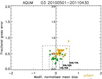
The MNMB and FGE can be combined in a “soccer” plot, which gives a convenient visual representation of the model error characteristics. In these plots (see Fig. 1 for an exam-ple) the MNMB is plotted on the x-axis, and FGE on the y-axis. Results for each station are plotted as a point. A perfect forecast would appear as a point at the origin, with the mag-nitude of any discrepancy increasing with distance from this point. Three boxes mark out maximum bias/error combina-tions of 15 %/35 %, 30 %/50 %, and 60 %/75 %: these val-ues are arbitrary, but have been selected as a convenient guide for visual interpretation of the plots. A systematic bias ap-pears as a linear grouping of points. If other random sources of error dominate, the resulting pattern will be a scatter of points. This representation is a convenient way of present-ing the statistics across a range of sites, with the quality of the overall forecast and any strong common characteristics or contrasts between the statistics at rural and urban sites be-ing immediately apparent.
An additional metric for comparing forecast and observa-tion fields is the Pearson correlaobserva-tion coefficient (R). This in-dicates the extent to which temporal patterns in the forecast match those in the observations at a single site or for an en-semble of sites. Another simple metric we use, which is con-venient for giving a broad-scale impression of overall fore-cast skill, is termed “FAC2”. This is the fraction of model
Fig. 1.Soccer plot showing fractional gross error as a function of the modified normalised mean bias relative to hourly observations of ozone for the period 1 May 2010 to 30 April 2011. Urban back-ground and suburban sites are shown in orange, while remote and rural sites are given in green.
predictions where the forecast value is within a factor of 2 (either greater or smaller) of the observed value.
3.2 Threshold exceedance skill scores
The verification measures described above provide informa-tion about the forecast errors under all condiinforma-tions, regardless of the magnitude of pollutant concentration. However, it is desirable to have metrics which provide information regard-ing forecast skill specifically at those times when pollutant levels are elevated and pose a greater risk to human health. It is important to assess the skill that models possess in pre-dicting exceedance of given thresholds. The odds ratio is con-structed from a standard 2×2 contingency table (Stephenson, 2000) and is defined as
θ=ad
bc, (5)
wherea is the number of correct forecasts of an event,bis number of false alarms,cis the number of missed forecasts andd is the number of correct rejections.
The odds ratio skill score (ORSS) can be constructed from the odds ratio via a simple transformation
ORSS=θ−1
θ+1. (6)
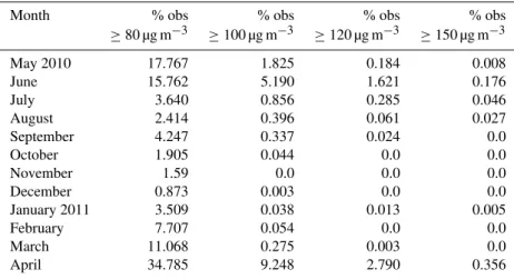
Table 1.Prevalence of ozone episode conditions by month between 1 May 2010 and 30 April 2011. For each month, the percentage of hourly average observations (across all sites) where the ozone concentration exceeds the given threshold is shown.
Month % obs % obs % obs % obs
≥80 µg m−3 ≥100 µg m−3 ≥120 µg m−3 ≥150 µg m−3
May 2010 17.767 1.825 0.184 0.008
June 15.762 5.190 1.621 0.176
July 3.640 0.856 0.285 0.046
August 2.414 0.396 0.061 0.027
September 4.247 0.337 0.024 0.0
October 1.905 0.044 0.0 0.0
November 1.59 0.0 0.0 0.0
December 0.873 0.003 0.0 0.0
January 2011 3.509 0.038 0.013 0.005
February 7.707 0.054 0.0 0.0
March 11.068 0.275 0.003 0.0
April 34.785 9.248 2.790 0.356
events occurring which were incorrect forecasts), defined as follows, are valuable metrics for assessing forecast perfor-mance:
H= a
a+c (7)
F = b
b+d. (8)
We have used an hourly average ozone concentration of 100 µg m−3as the threshold for defining an event in the
cat-egorical analyses conducted in Sect. 4. According to the cur-rent UK “Daily Air Quality Index”, an 8-h rolling mean value of this magnitude is the threshold for the designation of “moderate” levels of air pollution due to ozone.
Many of the above methods for characterising perfor-mance of air quality models were adopted by the GEMS project, based on a report by Agnew et al. (2007), where fur-ther discussion of verification issues is given.
4 Results of model evaluation
We have evaluated AQUM against hourly observations of O3, NO2, NO, PM10, and PM2.5 from the UK Automatic
Urban and Rural (AURN) observing network. Observations from around 70 rural, remote, urban background and subur-ban sites were used, although not all species are measured at every site. More information about the AURN for 2011 can be found in Stacey (2012), and similar reports for pre-vious years. The periods analysed are the 12-month period 1 May 2010–30 April 2011 and then the poor air quality episodes in July 2006, June 2010 and April 2011. In addition, we have analysed the period June to October 2011 to conduct a comparison of the operational AQUM forecasts with those of the MACC Regional Air Quality Ensemble.
4.1 Evaluation of one year of operational forecasts
4.1.1 Meteorology of May 2010–April 2011
The 12-month period was characterised by a climatologi-cally average start, followed by a relatively unsettled sum-mer 2010. Autumn started warm and settled, but ended cold, leading into an unusually cold December, followed by an av-erage January, and warm February and spring. The period ended with an exceptional spell of warm, settled weather for the time of year, with April 2011 being the warmest on record in the UK and also one of the sunniest and driest. More de-tails are available from the Met Office monthly weather sum-maries (Met Office, 2012).
4.1.2 Ozone
Ozone production and build up is favoured by strong sun-shine, light winds and elevated temperatures, and thus episodes of high ozone concentrations tend to be more fre-quent and severe in the summer. However, in the North-ern Hemisphere the background concentrations are gener-ally highest in the spring (Monks, 2000); this, together with enough insolation (necessary for regional ozone production) during those months, means that spring time ozone episodes are also frequently observed. The meteorology was not gen-erally favourable for ozone production in summer 2010, with cool, unsettled and overcast conditions. In fact, the highest levels of ozone during the period occurred during the ex-ceptionally warm April 2011, which saw around twice the frequency of elevated ozone compared to any other month (Table 1).
Model performance metrics for the forecasts during this 12-month period are shown in Table 2 for ozone (first col-umn). The model has a correlation coefficient with ob-servations of 0.68, a modest positive bias of 8.38 µg m−3,
Table 2.Model performance metrics for the period 1 May 2010– 30 April 2011. These statistics are based on all hourly values in each day. An ozone threshold of 100 µg m−3was used in the calculation of the ORSS, hit rate and false alarm rate metrics. The categorical metrics are presented only for ozone; these metrics add little value for interpreting the results for NO2and PM due to the large negative bias in model predictions for these species. The mean and standard deviation (SD) of observations and model values are also shown.
Metric O3 NO2 PM10 PM2.5
Correlation 0.68 0.57 0.52 0.53
Bias (µg m−3) 8.38 −6.10 −9.17 −3.41
RMSE (µg m−3) 22.80 18.66 17.28 12.89
MNMB 0.12 −0.26 −0.67 −0.30
FGE 0.49 0.69 0.83 0.62
FAC2 0.77 0.57 0.43 0.62
ORSS 0.95 * * *
Hit rate 0.57 * * *
False alarm rate 0.03 * * *
Mean observation (µg m−3) 46.75 22.23 19.51 14.42
Mean model (µg m−3) 55.13 16.13 10.34 11.01
SD observation (µg m−3) 24.84 21.29 16.79 13.61 SD model (µg m−3) 27.58 14.41 11.94 11.86
Number of sites 55 48 16 23
the observations. The false alarm rate for a threshold of 100 µg m−3is very low at only 3 % and the hit rate is 57 %.
The soccer plot for ozone at urban background (orange) and rural (green) stations is shown in Fig. 1. At urban stations the model has a positive bias, but there is no clear systematic bias for rural stations. Both bias and other sources of error con-tribute to the fractional gross error, and both are higher for the urban than the rural stations. These results will be interpreted in the following section in the context of the model’s perfor-mance for NOx. In Table 3 we present a summary of the
sea-sonal variation in model performance for ozone predictions. The highest seasonal values of the bias in modelled ozone (∼20 µg m−3)and of the hit rate for predicting exceedances
of the 100 µg m−3ozone threshold (0.84) are found in
sum-mer. The high bias observed during that season derives partly from the positive bias in the MACC LBCs (see Sect. 4.3) and partly due to overproduction/insufficient deposition within the model domain. A comparison of the variability in the model predictions (standard deviation of 27.58 µg m−3)with
that of observed values (standard deviation of 24.84 µg m−3)
shows that the model is able to reproduce well the observed variability in ozone concentrations over the course of a year. In Fig. 2 the diurnal variation in bias for ozone is shown. The bias peaks at 05:00 Z, reflecting the poor model skill in cap-turing the overnight ozone minimum. The main factors for this are likely to be limitations in the current model for rep-resenting stable nocturnal boundary layers, night-time chem-istry and NO2concentrations, discussed in the next section.
Fig. 2. Hourly variation of the mean ozone bias for the period 1 May 2010 to 30 April 2011.
Table 3.Seasonal variation of model performance metrics for ozone between 1 May 2010 and 30 April 2011. The mean and standard deviation (SD) of observations and model values are also shown.
Metric Spring Summer Autumn Winter
Correlation 0.63 0.65 0.65 0.72
Bias (µg m−3) 7.78 20.03 6.89 −0.41
RMSE (µg m−3) 24.45 26.69 20.41 19.19
MNMB 0.13 0.38 0.12 −0.12
FGE 0.41 0.42 0.50 0.61
FAC2 0.82 0.82 0.76 0.67
ORSS 0.86 0.97 0.99 1.00
Hit rate 0.46 0.84 0.62 0.23
False alarm rate 0.06 0.07 0.00 0.00
Mean observation (µg m−3) 57.96 48.66 40.99 39.30
Mean model (µg m−3) 65.74 68.68 47.88 38.89
SD observation (µg m−3) 25.55 20.84 21.82 24.86
SD model (µg m−3) 27.11 21.06 23.78 25.96
Number of sites 55 53 53 54
4.1.3 NO2
The model performance metrics for NO2are also shown in
Table 2. The correlation coefficient of 0.57 is lower than for ozone and there is a negative bias of−6.10 µg m−3which is
of a similar magnitude (but opposite in sign) to that of ozone. However, as NO2 concentrations are lower than ozone, the
magnitude of the MNMB is much greater, with values of 0.12 for ozone and−0.26 for NO2(corresponding toα=1.13 and
0.77, respectively).
Figure 3 shows the soccer plot for NO2. There is a large
negative bias at urban sites which dominates the overall error at these sites. At rural sites there is generally a positive bias, but the error displays a more random characteristic rather than the systematic trend for urban sites. It should be borne in mind that NO2 measurements made using the
Fig. 3. Soccer plot for NO2 for the period 1 May 2010 to 30 April 2011. Urban background and suburban sites are shown in orange, while remote and rural sites are given in green.
more than 50 %, depending on the concentrations of interfer-ing species, the distance from emission sources, and meteo-rological conditions (e.g. Dunlea et al., 2007; Steinbacher et al., 2007; Lamsal et al., 2008). Considering the lack of long-term simultaneous measurements of NO2using
chemilumi-nescence analysers equipped with molybdenum and pho-tolytic converters over the UK, and the uncertainties in the correction factors estimated from simulated concentrations of interfering species (see e.g. Lamsal et al., 2008, 2010), no attempt to correct for such interference has been made in this first evaluation of AQUM.
As a regional air quality model at ∼12 km resolution, AQUM does not adequately resolve the sources of primary NO and NO2emission (typically dominated by road
trans-port and combustion at point sources). In view of this we have not presented a systematic evaluation of model NO predictions. However, it is worthwhile noting that there is a strong negative bias for NO predictions which dominates the error characteristics. This pattern of over-estimation of NOxat rural sites and under-estimation at urban ones is
con-sistent with the model resolution being too coarse to prop-erly resolve sources of NOx. In an Eulerian model, primary
emissions are instantaneously spread over an entire grid box, thus giving apparently lower concentrations close to source regions than occur in reality. Corresponding with this, due to the overall conservation of emitted mass, there is a spuri-ous increase in concentrations at rural locations adjacent to source regions (urban centres or roads). These effects com-bine to give the pattern of biases observed for primary pol-lutants at rural and urban sites. This aspect of model per-formance is likely to improve as model resolution increases. The prediction of NO is expected to cause the under-estimation of the ozone loss by titration in the model, which
Fig. 4. Soccer plot for PM10 for the period 1 May 2010 to 30 April 2011. Urban background and suburban sites are shown in orange, while remote and rural sites are given in green.
is consistent with the positive bias found for this species at urban sites.
4.1.4 Particulate matter
The model performance statistics for PM10in Table 2 show
that overall it is the most challenging pollutant to model ac-curately. It has the lowest correlation coefficient (0.52) and the greatest negative bias (MNMB= −0.67), which implies that on average the model predictions for PM10are only half
of the observed concentrations; FGE (0.83) is also the high-est of all the pollutants.
Figure 4 shows the soccer plot for PM10. Urban sites
con-sistently have a negative bias and although there are few data available from rural sites, a negative bias is generally exhib-ited. The under-forecasting of concentrations of particulate matter is a widespread problem in most present-day forecast systems. Inspection of the MACC regional ensemble models (Moinat and Marecal, 2012) shows that all models exhibit a negative bias to some extent.
By contrast, the performance for PM2.5in AQUM is
sig-nificantly better, with MNMB= −0.30 and FGE=0.62 (see Table 2). PM2.5contains both primary and secondary
compo-nents, with the latter frequently dominating. An example is discussed in Sect. 4.2.3 where speciated PM measurements have allowed a more detailed analysis to be made. This dif-ference in model performance for PM10and PM2.5indicates
that most of the under-represented PM10is in the coarse
Fig. 5.Location of specific air quality observing sites in the UK referred to in the text and other Figures.
processes in the model which act on particles, such as dry deposition and transport, may also contribute to the errors in modelling PM10.
4.2 Model evaluation during pollution episodes
A key requirement of modelling and forecast systems is the ability to represent the rapid rise and fall of pollutant con-centrations which occur around episodes of poor air quality. Whilst most models can be tuned to give reasonable monthly or annual averages, a more discriminating test is whether models can respond in episode conditions and demonstrate a wide dynamic range, predicting the onset and termination of elevated pollutant concentrations. To assess this aspect of model performance, it is helpful to compare the variability in model predictions with the variability in observed concentra-tions for a given pollutant. In the next two secconcentra-tions we assess the performance of the model during periods of moderate and high, ozone and PM: June 2010 and April 2011 as well as the additional month of July 2006, which was modelled in hind-cast mode. The geographical locations of particular sites for which we show results are depicted in Fig. 5.
4.2.1 July 2006
This month was exceptionally warm and sunny and there-fore produced some of the most significant ozone episodes
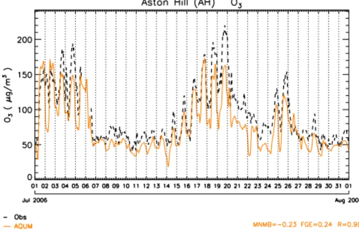
Fig. 6.Time series of hourly ozone concentrations (µg m−3)for the rural site at Aston Hill, for July 2006. Observed concentrations are shown as the black dashed line and the model output as the solid orange line.
that the UK has experienced since 2003. Consequently, this month is a demanding test of the model because ozone levels were particularly high at their peak and because the ozone episodes came in separate phases. There were three signif-icant ozone episodes, separated by days when ozone levels were low. This period is therefore a good test of the model’s dynamic range in modelling the rapid build-up of ozone, the maintenance of high levels during the episode and the reduc-tion at the end.
Figure 6 shows modelled and observed hourly ozone for Aston Hill, a rural site on the border between England and Wales. At this site there were three ozone episodes: an ini-tial one from the 1st to the 5th July, a second one from the 17th to the 20th and a third more modest episode cover-ing 24–25 July. For this site the model exhibits a negative bias, but generally reproduces well the pattern of the ob-servations throughout the month, both in terms of predict-ing actual ozone levels and episode duration. However, it did not predict the highest concentration occurring on the 19 July. The low values of ozone between the episodes are well reproduced, showing that the model is able to capture abrupt changes in ozone concentration as episode condi-tions arise and then dissipate. Similar results were found for most rural and urban sites. The summary performance statis-tics are given in Table 4. Although the bias for this month (1.99 µg m−3)is particularly low compared to that of summer
2010 (20.03 µg m−3, see Table 3), the RMSE remains similar.
Table 4.Model performance metrics for ozone for the three case study periods, July 2006, June 2010 and April 2011. An ozone threshold of 100 µg m−3was used in the calculation of the ORSS, hit rate and false alarm rate metrics. The mean and standard devia-tion (SD) of observadevia-tions and model values are also shown.
Metric July 2006 June 2010 April 2011
Correlation 0.75 0.66 0.59
Bias (µg m−3) 1.99 20.37 7.09
RMSE (µg m−3) 25.94 28.26 24.89
MNMB 0.07 0.33 0.14
FGE 0.31 0.38 0.35
FAC2 0.89 0.86 0.86
ORSS 0.92 0.95 0.80
Hit rate 0.71 0.86 0.43
False alarm rate 0.09 0.14 0.08
Mean observation (µg m−3) 68.94 57.17 66.66
Mean model (µg m−3) 70.93 77.54 73.73
SD observation (µg m−3) 38.47 23.01 28.05
SD model (µg m−3) 33.96 24.16 23.87
Number of sites 54 53 54
A key requirement for a forecast system is to be able to predict ozone concentration levels greater than a given threshold. Using a threshold of 100 µg m−3, Table 4 also
shows the categorical metrics (hit rate, false alarm rate, ORSS) for July 2006. The hit rate is high for July 2006 (0.71). In view of the fact that there is a low positive bias, this demonstrates that the model predicts this episode well, al-though the variability in model predictions (33.96 µg m−3)is
not quite as large as that in observed values (38.47 µg m−3).
It should also be noted that the hit rate is very sensitive to the threshold chosen and to the overall pollution levels during a given episode, as found in our analysis of April 2011 (see Sect. 4.2.3).
4.2.2 June 2010
The weather over the UK in June 2010 was mainly dry and sunny, particularly in the second half when it became very warm, reaching a maximum of 30.9◦
C in Gravesend (South East England) on 27 June. Although sunshine levels were below average in Scotland, they were around 50 % above av-erage in South Wales and South West England, where it was the third sunniest June since 1929. The majority of the rain-fall occurred during the second week, and it became unsettled again at the very end of the month (Met Office, 2010).
There were two main poor air quality episodes this month, with high levels of both ozone and PM10. The first period
was from 3 to 6 June, during which elevated levels of all the key air quality pollutants were observed across southern Eng-land, with ozone reaching a maximum of 172 µg m−3at
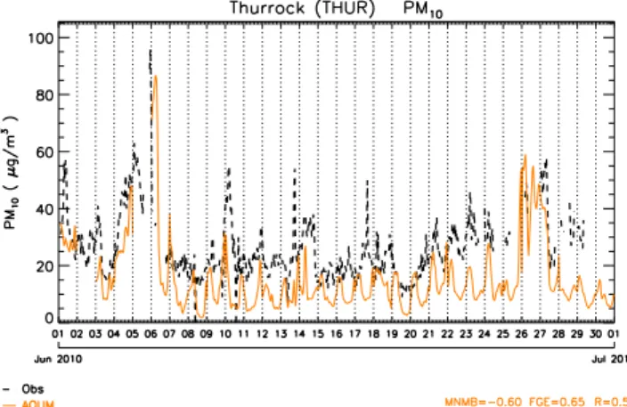
Wey-bourne on the 6th. PM10peaked at 96 µg m−3in Thurrock on
the 5th (see Fig. 7). The model captures this first episode well, both in timing and in magnitude. There were other short-lived, smaller magnitude peaks of PM throughout the
Fig. 7.Time series of hourly PM10concentrations (µg m−3)for the urban background site at Thurrock, east of London, for June 2010. Observed concentrations are shown as the black dashed line and the model output as the solid orange line.
month which the model did not capture so well and overall the model exhibited a negative bias. A determination of the precise reasons for the model’s ability to capture some peaks but not others would require a more detailed analysis than is possible at the present time. From 22 to 28 June a longer du-ration episode occurred. During this episode PM10 reached
a maximum of 89 µg m−3 in Leamington Spa on the 28th,
while a peak value of ozone was recorded in Weybourne on the 27th, at a concentration of 194 µg m−3; 40 other sites
observed peak ozone concentrations of above 100 µg m−3
and of these, 6 sites measured ozone concentrations higher than 150 µg m−3. Figure 8 shows the time series of ozone
concentrations for the Harwell site (a rural location around 30 miles west of London) and illustrates the extent of the episode. Here the model captures the general characteristics and higher peak concentrations of the episode well. This is reflected in the high ORSS score of 0.95. The ozone predic-tion performance statistics for the whole month are shown in Table 4. For the month overall, the variability in model predictions (24.16 µg m−3)slightly exceeds that in observed
values (23.01 µg m−3).
A contour plot showing the daily maximum values of ozone across the model domain is shown for 27 June in Fig. 9. In this figure the observed daily maxima are over-plotted as colour-coded squares. It can be seen that the model predicts ozone levels higher than 150 µg m−3 across
a large swathe of south-eastern England, compared to ob-served concentrations, where only two sites – Weybourne and Sibton – actually reached these levels. This trend to over-forecast ozone levels is continued across the entire month, as indicated by the relatively large positive model bias of 20.37 µg m−3 (see Table 4) for the thirty day period. This
Fig. 8.Time series of hourly ozone concentrations (µg m−3)for the rural site Harwell for June 2010. Observed concentrations are shown as the black dashed line and the model output as the solid orange line.
4.2.3 April 2011
The meteorology of May 2010–April 2011 was not generally conducive to the build-up of ozone, with the summer lacking extended periods of clear skies and high temperatures. In-stead, a period of elevated ozone occurred during April 2011, which was unusually warm and sunny. The combination of these conditions with the elevated background concentra-tions noted above resulted in some of the poorest air qual-ity over the UK for the whole of 2011. The elevated ozone levels occurred together with a major PM episode. Meteoro-logically, high pressure dominated the UK weather through-out the month, resulting in mainly fine, warm weather. Daily maximum temperatures were well above normal – by as much as 6◦
C in South East England, with a maximum of 27.8◦
C recorded in Wisley, Surrey, on 23 April. It was also one of the driest and sunniest months of April on record, although Scotland had near to above normal rainfall (Met Office, 2011).
There were widespread elevated ozone levels which peaked during the period 20th–23rd. Due to the contribution of background ozone levels the onset of the episode is not especially pronounced, as demonstrated by the time series for Harwell shown in Fig. 10, where ozone levels were gen-erally high throughout the month. Table 4 shows the model performance characteristics for April 2011 for ozone. While the bias and RMSE are generally comparable to the other episodes, the hit rate is significantly lower. This is likely to be because the ozone concentrations were close to the thresh-old value for much of April, so that small errors in the model forecast concentration values could often result in incorrect classification as a hit or false alarm.
The most notable feature for April 2011 was the major PM episode which occurred from approximately 18 to 23 April
Fig. 9.Maximum modelled hourly ozone concentrations (µg m−3) for 27 June 2010, with observed concentrations over-plotted within squares.
and affected the whole of the UK. A maximum PM10
concen-tration of 142 µg m−3was observed in Thurrock on 21 April
(see Fig. 11). AQUM predicts the overall evolution of the episode well, but under-predicts the observed concentrations on the three days which saw the maximum PM10levels. This
episode illustrates that when PM10 is dominated by the
for-mation of PM2.5 secondary aerosol, AQUM predictions of
the former improve. Speciated PM observations are avail-able for this episode at the rural Harwell site (S. Telling, per-sonal communication, 2011). A time series plot of measured PM2.5 and its components at this site is shown in Fig. 12.
On 22 April PM10at Harwell reached a maximum
concen-tration of 105 µg m−3; most of this was in the PM
2.5
compo-nent with a concentration of 98 µg m−3. The largest
compo-nent of PM2.5was nitrate aerosol, with a peak concentration
of 56 µg m−3. The modelled speciated PM
2.5concentrations
are shown in Fig. 13 for comparison with the observations. AQUM correctly predicts the overall magnitude of PM2.5and
Fig. 10.Time series of hourly ozone concentrations (µg m−3)for the rural site at Harwell, for April 2011. Observed concentrations are shown as the black dashed line and the model output as the solid orange line.
Fig. 11. Time series of hourly PM10concentrations (µg m−3)for the urban background site of Thurrock, east of London at the peak of the April 2011 episode. Observed concentrations are shown as the black dashed line and the model output as the solid orange line.
aerosol components. However, the model does not predict the worsening of PM2.5values from the 20th to the 22nd and
sig-nificantly over-predicts values on 23rd April and other days.
4.3 Sensitivity to chemical LBCs
AQUM has a relatively small domain, hence model predic-tions can be expected to exhibit sensitivity to the chemical LBCs. We have assessed this sensitivity of model ozone pre-dictions in two ways: (i) by running AQUM with two inde-pendent LBC datasets and (ii) by adding an intermediate Eu-ropean nested domain and evaluating the changes in AQUM performance.
Fig. 12.Speciated PM2.5measurements at the rural site Harwell for the peak of the April 2011 episode.
4.3.1 Model comparison using independent LBC datasets
Both the GEMS and MACC projects produced global model chemical reanalyses. These reanalyses were conducted with different model configurations and resulted in two indepen-dent datasets which were used to derive chemical LBCs for AQUM. The model was re-run for the whole of 2006 us-ing both sets of LBCs. An example time series of hourly ozone predictions at the rural Yarner Wood station is shown in Fig. 14. From January to May simulations made with the GEMS LBCs exhibit a larger negative bias than those made with the MACC LBCs; from May to the end of the year runs using the GEMS LBCs generally perform better, with a smaller positive bias. Plots for other sites show the same general behaviour. These results are consistent with the known negative bias in lower tropospheric ozone from the GEMS reanalysis during the first quarter of 2006 (Schere et al., 2012) and illustrate the sensitivity of AQUM predictions to the LBCs used. The question then arises as to whether this sensitivity can be reduced by using an intermediate nest on a larger domain.
4.3.2 Impact of intermediate nest
Fig. 13.Speciated PM2.5model forecasts for the rural site Harwell for the peak of the April 2011 episode.
Fig. 14.Comparison of a year-long run of AQUM for 2006: results for ozone at the rural site Yarner Wood using LBCs from GEMS (orange) and MACC (green) reanalyses.
– AQUM-GEMS and AQUM-MACC: these refer to the standard domain of AQUM driven with either GEMS or MACC global model LBCs.
– EU-GEMS and EU-MACC: these refer to the Euro-pean domain driven with either GEMS or MACC global model LBCs.
– EUUK-GEMS and EUUK-MACC: these refer to the 3-level nested configuration of the standard AQUM do-main driven by LBCs from the European dodo-main, which is in turn driven with either GEMS or MACC global model LBCs.
These additional model configurations were run for June and July 2012. Figure 16 shows a time series at the Har-well site for AQUM-GEMS, EU-GEMS and EUUK-GEMS.
Fig. 15.Location of the intermediate European domain used to eval-uate sensitivity to LBCs.
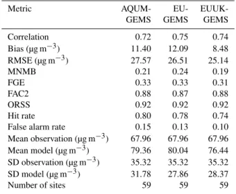
Fig. 16.Time series of ozone at the rural site Harwell comparing AQUM-GEMS, EU-GEMS and EUUK-GEMS model configura-tions for 2 June to 29 July 2006.
Table 5.Model performance metrics for ozone for the three model configurations AQUM-GEMS, EU-GEMS, EUUK-GEMS for the period 2 June to 29 July 2006.
Metric AQUM- EU-
EUUK-GEMS GEMS GEMS
Correlation 0.72 0.75 0.74
Bias (µg m−3) 11.40 12.09 8.48
RMSE (µg m−3) 27.57 26.51 25.14
MNMB 0.21 0.24 0.19
FGE 0.33 0.33 0.31
FAC2 0.88 0.87 0.88
ORSS 0.92 0.92 0.92
Hit rate 0.80 0.78 0.74
False alarm rate 0.15 0.13 0.10
Mean observation (µg m−3) 67.96 67.96 67.96
Mean model (µg m−3) 79.36 80.04 76.44
SD observation (µg m−3) 35.32 35.32 35.32
SD model (µg m−3) 31.78 27.86 28.37
Number of sites 59 59 59
4.4 Comparison with the MACC regional air quality ensemble
MACC was a project funded under the European Union Sev-enth Framework Programme FP7 to develop and implement trial elements of an atmospheric composition and climate ser-vice. One element of MACC is a European air quality fore-cast service. Seven different models forefore-casting for a Euro-pean domain contribute to an ensemble median forecast out to three days ahead. In order to place the performance of AQUM in the context of other similar air quality forecast models we have conducted a comparison between AQUM and the MACC ensemble forecast over the period June to October 2011.
Summer 2011 was generally cooler and slightly wetter than average, and in particular it was wetter than 2010. How-ever, there were some periods of fine weather, and the last few days of September and the first week in October were very warm and sunny for this time of year. There were several periods of elevated ozone during June–October: in both early and late July as well as at the end of September and early Oc-tober. Both AQUM and the MACC ensemble captured these events fairly well (see, for example, a time series of ozone daily maximum at Harwell in Fig. 17). The times series plot in Fig. 18 compares the hourly ozone concentration bias for the MACC ensemble and AQUM. In general, AQUM has a higher bias than the MACC ensemble, with mean values over the whole period of 13.28 µg m−3for AQUM compared to
4.10 µg m−3for the MACC ensemble. This figure illustrates
that the positive bias of both model systems rises during the episode periods. Table 6 shows a summary of performance metrics. The performance of the MACC ensemble is some-what better than that of AQUM for most metrics, but AQUM
Fig. 17.AQUM and MACC ensemble predictions of daily maxi-mum ozone concentrations compared to observations at the rural site Harwell for 1 June to 31 October 2011. The observations are the black dashed line, AQUM output in orange and MACC ensem-ble predictions in green.
has a notably higher hit rate (for the 100 µg m−3ozone
con-centration threshold) and a range of variability (given by the standard deviation) closer to that of the observations. Consid-ering mean value metrics such as bias and RMSE, one would expect the ensemble performance of a collection of well-configured models to be better than that of any single mem-ber, hence the greater skill of the ensemble forecast as indi-cated by these metrics is not surprising. However, the hit rate of AQUM at 0.64 is significantly better than the value of 0.27 achieved by the MACC ensemble. The contributing factors for this difference are likely to be (i) the “smoothing” effect of taking the median value of the MACC ensemble, which excludes the higher magnitude forecasts and (ii) the higher bias of AQUM. For a forecast model designed for issuing health impact warnings, the higher hit rate is arguably a more important characteristic than a lower bias, as long as the false alarm rate does not increase unacceptably as a result. The false alarm rate for AQUM is only 4 %, whilst the MACC ensemble has no false alarms. Finally, the lower range of variability in the MACC ensemble (∼17.6 µg m−3 standard
deviation) compared to the AQUM forecast (∼21.3 µg m−3)
and the observations (∼21.0 µg m−3)might also be related to
the “smoothing” effect of the ensemble.
4.5 Variation of model skill with forecast lead time
Fig. 18.Time series of hourly ozone bias for AQUM operational output in orange and MACC ensemble in green.
Table 6.Performance metrics for AQUM and MACC ensemble ozone forecasts for the period 1 June to 31 October 2011. The small differences in the means and standard deviations of the observations used for evaluating AQUM and the MACC ensemble are due to mi-nor variations in data availability over the period.
Metric AQUM MACC Ensemble
Correlation 0.62 0.71
Bias (µg m−3) 13.28 4.10
RMSE (µg m−3) 22.66 15.71
FAC2 0.85 0.89
ORSS 0.96 0.99
Hit rate 0.64 0.27
False alarm rate 0.04 0.0
Mean observation (µg m−3) 44.71 47.75
Mean model (µg m−3) 60.99 51.85
SD observation (µg m−3) 21.04 21.09
SD model (µg m−3) 21.29 17.55
Number of sites 60 60
variables, where one generally finds a significant decrease in forecast skill with lead time, ozone forecasts exhibit a weak dependence on lead time for all metrics. This is consistent with our general observation that, for air quality forecasting, a 24-h persistence forecast (i.e. assuming the next day has the same air quality as the current day) usually exhibits a sub-stantial level of skill. The contrasting behaviour with meteo-rological forecasts indicates that the factors controlling errors differ in the two types of forecast, and that the impact of typi-cal errors in meteorology does not dominate other sources of error in ozone forecasts, such as emissions or the representa-tion of atmospheric chemistry.
Table 7.AQUM performance metrics for ozone forecasts over the period 1 May 2010 to 30 April 2011, illustrating variation with fore-cast lead time. The small differences in the means and standard de-viations of the observations used for evaluating forecasts are due to minor variations in data availability over the period.
Metric Day 1 Day 2
Correlation 0.68 0.66
Bias (µg m−3) 8.38 9.04
RMSE (µg m−3) 22.80 23.79
FAC2 0.77 0.76
ORSS 0.95 0.95
Hit rate 0.57 0.56
False alarm rate 0.03 0.04
Mean observation (µg m−3) 46.75 46.77 Mean model (µg m−3) 55.13 55.81 SD observation (µg m−3) 24.84 24.94 SD model (µg m−3) 27.58 27.70
Number of sites 55 55
5 Summary and future developments
We have presented a description of a new on-line air qual-ity model AQUM, which is based on the Met Office Unified Model and uses the UKCA sub-model for describing atmo-spheric chemistry processes. A variety of metrics for assess-ing model performance have been described and the impor-tance of using metrics which assess both mean performance and skill in predicting exceedance of threshold concentra-tion values is emphasised. We have evaluated AQUM against routine, hourly observations from the UK AURN surface ob-serving network. Averaged over the course of a full year, the model exhibits a positive bias for ozone of around 8 µg m−3.
The model exhibits good dynamic range in simulating ozone, as shown by the fact that the variability in model predictions over the course of a year is comparable to, or exceeds, the variability in observed values. Case studies of elevated ozone episodes demonstrate that the model reproduces time series of measured ozone concentrations at individual sites well. For NO2 the model exhibits a negative bias for urban sites
and positive bias for rural sites. This is likely to be a con-sequence of the fact that, at 12-km resolution, AQUM does not adequately resolve the main sources of NOx (i.e. road
traffic and combustion point sources). This results in the di-lution of emissions close to source regions (urban areas) and enhanced emissions in regions distant from sources (rural ar-eas). For PM10the model generally exhibits a negative bias
(as discussed in Sect. 4.1.4.), in common with many air qual-ity models. However, the model performance for PM2.5 is
better, with a much smaller negative bias. During particular PM episodes where secondary inorganic aerosols dominate, such as April 2011, PM10performance improves. The lower
skill exhibited for PM10 is likely to be the result of
in the annual average inventories, such as re-suspension of deposited coarse PM, sea salt or wind blown dust.
The sensitivity of modelled ozone to chemical LBCs has been assessed by taking these from two different global re-analyses and by comparing the standard, single-nested con-figuration with another concon-figuration having an intermedi-ate European nest. We conclude that, even with a much larger regional domain, the LBCs remain an important source of model error for relatively long-lived pollutants such as ozone. The AQUM forecast for ozone has also been com-pared to the median of the MACC ensemble and overall the latter exhibits better performance as judged by mean field metrics. However, it has a significantly lower hit rate for pre-dicting exceedance of the 100 µg m−3 ozone concentration
threshold and somewhat lower variability compared to that of AQUM and the observations.
AQUM is being actively developed by the Met Office and UKCA academic partners. Priority areas for future develop-ments include:
i. An improved representation of emissions. At present, monthly data from three emission inventories (EMEP, NAEI and ENTEC) are interpolated to the AQUM hor-izontal grid and merged. These data, which originate from different source sectors, are aggregated as a sin-gle surface emission field for most species. In the case of gas phase emissions, such 2-dimensional fields have been spread over the four lowest model levels in this study. Temporal factors accounting for day of week and hour of the day have also been applied based on UK data. A more comprehensive system is currently being developed which will enable separate vertical and tem-poral profiles to be applied according to source sectors. Different options are being considered for the allocation of emissions in the model layers such as the use of ver-tical profiles according to a default distribution based on SNAP sectors (Vidic, 2002) or effective emission heights calculated by more recent studies (e.g. Pregger and Friedrich, 2009; Bieser et al., 2011). Our current time profiles will also be evaluated against new tempo-ral emission factors (e.g. Menut et al., 2012) and up-dated if needed. Finally, recent developments in UKCA will enable the use of interactive emissions of biogenic VOCs. The new framework will also allow us to more easily interface new or improved treatments of biomass burning and soil emissions.
ii. Replacement of the mass-based CLASSIC aerosol scheme by the modal aerosol microphysics scheme “UKCA-GLOMAP-mode” (Mann et al., 2010). This more sophisticated scheme will allow the time evo-lution of aerosol modes, the separate modelling of aerosol mass and number, the representation of in-ternally mixed particles, the inclusion of microphys-ical processes such as nucleation, a better coupling with UKCA oxidants, and an improved representation
of sea salt and prognostic secondary organic aerosols. Currently, the fact that the CLASSIC aerosol scheme treats the sulphur chemistry in a separate module to the rest of the gas phase chemistry also makes it dif-ficult to treat from the emissions perspective and in-troduces the potential for inconsistencies in the chem-ical mechanism; this will be overcome with the use of the more consistent UKCA-GLOMAP-mode scheme in which the sulphur chemistry is an intrinsic part of the chemical mechanism and emissions of all gases and aerosols are dealt with in the same framework. The analysis of global model simulations using both schemes shows that UKCA-GLOMAP-mode compares better than CLASSIC against a global aerosol reanaly-sis and aerosol ground-based observations (Bellouin et al., 2012).
iii. The implementation of a post-processing system to ap-ply a bias correction to forecasts. The observation that a 24-h persistence forecast for air quality generally dis-plays considerable skill suggests that measured values from the previous 24-h period can be used to derive a bias correction to new forecasts. We have begun devel-opment work to explore the potential of this and initial results appear promising.
iv. A final priority for development is to increase the model resolution. The Met Office currently runs a 1.5-km res-olution, 70-level meteorological model which resolves smaller scale convection and gives an improved forecast for precipitation. In the near future we plan to develop a version of AQUM at 4-km resolution, reducing ulti-mately to 1.5 km in line with the meteorological fore-cast model. In addition to providing improvements in the meteorological parameters in AQUM, this will al-low an improved representation of concentration gradi-ents in pollutants, giving higher concentrations of pri-mary pollutants in urban areas and lower values in the rural areas close to cities.
Supplementary material related to this article is available online at: http://www.geosci-model-dev.net/6/ 353/2013/gmd-6-353-2013-supplement.pdf.
Copyright Statement