Ocean Sci., 12, 825–842, 2016 www.ocean-sci.net/12/825/2016/ doi:10.5194/os-12-825-2016
© Author(s) 2016. CC Attribution 3.0 License.
Major improvement of altimetry sea level estimations using
pressure-derived corrections based on ERA-Interim
atmospheric reanalysis
Loren Carrere, Yannice Faugère, and Michaël Ablain
Collecte Localisation Satellites, Parc Technologique du Canal, 8–10 rue Hermès, 31520 Ramonville-Saint-Agne, France Correspondence to:Loren Carrere ([email protected])
Received: 22 December 2015 – Published in Ocean Sci. Discuss.: 18 January 2016 Revised: 12 May 2016 – Accepted: 23 May 2016 – Published: 27 June 2016
Abstract. The new dynamic atmospheric correction (DAC) and dry tropospheric (DT) correction derived from the ERA-Interim meteorological reanalysis have been computed for the 1992–2013 altimeter period. Using these new corrections significantly improves sea level estimations for short tempo-ral signals (< 2 months); the impact is stronger if considering old altimeter missions (ERS-1, ERS-2, and Topex/Poseidon), for which DAC_ERA (DAC derived from ERA-Interim me-teorological reanalysis) allows reduction of the along-track altimeter sea surface height (SSH) error by more than 3 cm in the Southern Ocean and in some shallow water regions. The impact of DT_ERA (DT derived from ERA-Interim meteo-rological reanalysis) is also significant in the southern high latitudes for these missions.
Concerning more recent missions (Jason-1, Jason-2, and Envisat), results are very similar between ERA-Interim and ECMWF-based corrections: on average for the global ocean, the operational DAC becomes slightly better than DAC_ERA only from the year 2006, likely due to the switch of the opera-tional forcing to a higher spatial resolution. At regional scale, both DACs are similar in the deep ocean but DAC_ERA raises the residual crossovers’ variance in some shallow wa-ter regions, indicating a slight degradation in the most recent years of the study. In the second decade of altimetry, unex-pectedly DT_ERA still gives better results compared to the operational DT.
Concerning climate signals, both DAC_ERA and DT_ERA have a low impact on global mean sea level rise (MSL) trends, but they can have a strong impact on long-term regional trends’ estimation, up to several millimeters per year locally.
1 Introduction
Since the 1990s, several altimeter missions have been mon-itoring the sea level at a global scale. Thanks to its cur-rent accuracy and maturity, altimetry is now considered as a fully operational and accurate observing system dedicated to scientific and operational applications, among which un-derstanding the global climate change and the related global mean sea level rise (MSL) and mesoscale applications are a priority.
Satellite altimetry has shown its efficiency in detecting early changes in the global and regional MSL trends (Willis and Church, 2012; Cazenave et al., 2014). However, ensuring the long-term consistency and stability of altimeter measure-ments from one or several missions is challenging.
The global MSL trend has been determined to be around 3.2 mm yr−1over the period 1993–2008, with an uncertainty
of 0.5 mm yr−1(Ablain et al., 2009, 2015) mostly explained
by the orbit errors (Couhert et al., 2014), the aging of the al-timeters’ instruments, the drifts detected in radiometer wet tropospheric correction (Legeais et al., 2014), and uncertain-ties due to geophysical corrections.
In order to access the targeted ocean signal, altimeter mea-surements are corrected from several instrumental and geo-physical corrections including the dry tropospheric correc-tion (DT), and the dynamic atmospheric correccorrec-tion (DAC) which is one of the most critical after the tide correction.
Willebrand et al., 1980), taking into account that a DAC in-stead of a static inverse barometer correction (IB) allowed a very significant improvement of the altimetry product (Car-rere and Lyard, 2003). Then, the quality of the DAC has in-creased from 2007 thanks to a better bathymetry field and a higher-resolution mesh (Carrere et al., 2007). Still, signifi-cant errors remain mostly due to a lack of resolution of the model (in shelf seas but also in some deep ocean regions), to remaining bathymetry errors and also due to atmospheric forcing field uncertainties (Lamouroux et al., 2006; Lam-ouroux, 2006; Greenberg et al., 2007).
In this context, the main objective of the sea level CCI project (Ablain et al., 2015) was to build improved long-term altimeter sea level data records dedicated to climate studies. For that purpose, several algorithms (instrumental parame-ters, orbit calculation, radiometer wet tropospheric correc-tion, atmospheric corrections derived from model, oceanic tidal corrections, sea state bias, etc.) were developed to im-prove altimetry data and the processing to merge altimeter missions together.
Concerning the pressure-derived DAC and DT corrections, one of the main issues comes from the fact that the ECMWF operational analyses used to force the barotropic model are not compliant with climate and MSL applications. The sta-bility is not ensured because many jumps exist in the mete-orological temporal series due to ECMWF model evolutions or upgrades; Ablain et al. (2009) showed a significant impact of these jumps on the trends of the IB and the dry tropo-spheric corrections which both depend on the atmotropo-spheric pressure field. Moreover, the quality of the operational mete-orological data set is not homogeneous for the entire altime-ter period: early years are less accurate because of the use of old versions of the analysis system (ECMWF, 2016) and this may impact the estimation of mesoscale signals for the oldest years (Carrere, 2003).
The methodology adopted is to use the ERA-Interim me-teorological reanalysis (Dee et al., 2011) to compute the new corrections (hereafter, DAC_ERA and DT_ERA) and ana-lyze their impact on sea level estimation at climate scales, as well as at lower temporal scales for mesoscale applications. The main advantage of using meteorological reanalysis is the homogeneous quality of the temporal series, but at the cost of a lower spatial resolution.
After a complete description of the data sets and the meth-ods of comparison in Sect. 2, we present an analysis of the differences of the atmospheric pressure-derived correc-tions in Sect. 3, and the impact of the new DAC_ERA and DT_ERA corrections on ocean short-scale signals in Sect. 4. Section 5 is dedicated to ocean long-term climate signals and Sect. 6 gathers the discussion and concluding remarks.
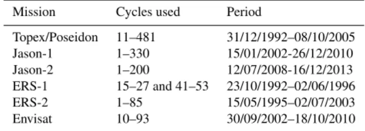
Table 1.Cycles used for the analysis of each altimeter mission.
Mission Cycles used Period
Topex/Poseidon 11–481 31/12/1992–08/10/2005 Jason-1 1–330 15/01/2002-26/12/2010 Jason-2 1–200 12/07/2008-16/12/2013 ERS-1 15–27 and 41–53 23/10/1992–02/06/1996 ERS-2 1–85 15/05/1995–02/07/2003 Envisat 10–93 30/09/2002–18/10/2010
2 Description of the data sets and method 2.1 Altimeter data
The altimeter measurements used were produced by Ssalto/Duacs and are distributed by Archiv-ing, Validation, Interpretation of Satellite Oceano-graphic data (AVISO, 2011), with support from CNES (http://www.aviso.altimetry.fr/en/data/products/ sea-surface-height-products/global.html). Particularly, we have considered level 2 altimetric products, with 1 Hz along-track resolution, usually called geophysical data records (GDRs).
The altimeter period (from 1993) is sampled by six al-timeter missions available on two different long-term tracks: TOPEX/Poseidon (TP in the text and in figures), Jason-1 (J1 in the figures), and Jason-2 (J2 in the figures), which are the reference missions flying on the reference TP track with a 10-day cycle; and ERS-1 (E1 in the figures), ERS-2 (E2 in the figures), and Envisat (EN in the figures), which fly on a sun-synchronous orbit with a 35-day cycle. The cycles used for the present study are listed in Table 1.
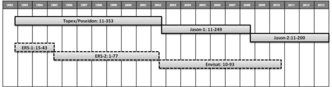
The different missions have been homogenized (Ablain et al., 2015) and the temporal series of TP, 1, and Jason-2 on one hand, and ERS-1, ERS-Jason-2, and Envisat on the other hand, have been concatenated to produce two long-term al-timeter time series as described in Fig. 1. Nearly 20 years of data for each different orbit have been used for the present study, from 1993 onwards.
The altimeter sea surface height (SSH) is defined as the difference between orbit and range, corrected from several instrumental and geophysical corrections:
SSH = orbit−range−DAC−DT−tide−other_corr where
– DAC is the dynamic atmospheric correction studied in this paper; DT is the dry tropospheric correction also studied in this paper.
L. Carrere et al.: Major improvement of altimetry sea level estimations 827
Figure 1.Altimeter long-term time series used in the study.
– Other_corr includes the wet tropospheric correction, the ionospheric correction, the sea state bias correction, and complementary instrumental corrections if needed.
– The sea level anomaly (SLA) is defined by the differ-ence between SSH and a mean profile (MP) for repeti-tive orbits or a mean sea surface (MSS) for drifting or new orbits. Mean profiles computed for the reference period of 7 years (1993–1999), respectively for TP– Jason and ERS–Envisat orbits, have been used for the present study (Hernandez and Schaeffer, 2001). 2.2 ERA-Interim data set
The ERA-Interim meteorological data set is the latest global atmospheric reanalysis produced by the European Centre for Medium-Range Weather Forecasts (ECMWF). Nearly 34 years of data (from 1 January 1979) are available on the N128 Gaussian grid (equivalent to∼0.7◦), which is the native reso-lution chosen for the reanalysis. More details about the con-figuration and the performances of the system are given in the ERA-Interim reanalysis report (Dee et al., 2011). When compared to the ECMWF operational analysis, ERA-Interim benefits from a constant resolution and a constant model ver-sion which makes it very useful for climate studies in par-ticular. ERA-Interim resolution is better than the operational one on the first years of altimetry (0.7◦instead of 1◦).
Six-hourly ERA-Interim analysis grids of sea level pressure and 10 m wind speeds have been used for the study.
2.3 The dynamic atmospheric correction
The high-frequency (HF) ocean signal forced by the atmo-sphere has a strong variability and is mostly located at high latitudes and in shallow water regions (Willebrand et al., 1980; Mathers, 2001); it is mostly barotropic if considering large spatial scales (Vinogradova et al., 2007). This HF sig-nal is aliased into the lower-frequency band due to the bad temporal sampling of satellite altimeters (time revisit of 10 days for TP–Jason altimeters); if not corrected, this signal thus pollutes ocean circulation estimations from altimetry for mesoscale or climate applications and also for satellite calibration campaigns. This HF ocean variability thus needs
to be corrected from an independent geophysical correction with centimetric accuracy (Stammer et al., 2000).
Since 2004, the dynamic atmospheric correction is used in altimeter GDRs; it is a combination of the high frequencies of MOG2D-G barotropic model forced by pressure and wind (Carrere, 2003) and the low frequencies (LF) of the inverted barometer, assuming a static response of the ocean to atmo-spheric forcing for low frequencies. The filtering wavelength is based on the TP/Jason-1/Jason-2 Nyquist frequency of 20 days (twice a cycle length), because this correction is pri-marily a de-aliasing correction made for reference altimeter missions (Carrere and Lyard, 2003).
DAC=MOG2D-GHF(T≤20 days)+IBLF(T >20 days) (1) As far as ERS and Envisat missions are concerned, the sam-pling Nyquist period is 70 days which means that the DAC does not remove all atmospheric forced high-frequency sig-nals aliased in the data. For altimeter multi-mission prod-ucts (AVISO, 2011), remaining aliased signals are smoothed thanks to a long wavelength error correction; however, for mono-mission products like GDRs, these signals remain aliased in lower-frequency signals and can interfere with cli-mate/seasonal variability (Carrere et al., 2010).
The reference DAC correction is computed from the 6 h ECMWF operational analysis (sea level pressure and 10 m winds) as done in CNES/AVISO data set (AVISO, 2011; Car-rere and Lyard, 2003). The reference DAC is DAC_ECMWF hereafter.
2.3.1 Processing of S1 and S2 atmospheric tides As far the dynamic atmospheric correction for altimetry is concerned, the diurnal (S1) and semidiurnal (S2) atmo-spheric tides demand a specific processing because they gen-erate radiational tides at the same frequencies of the diurnal and semidiurnal ocean tides. As the radiational and the grav-itational components cannot be well separated from obser-vations, both components are included in global ocean tide models; thus, the radiational tides should not be also included in the DAC correction to avoid redundancy when correcting altimetry data.
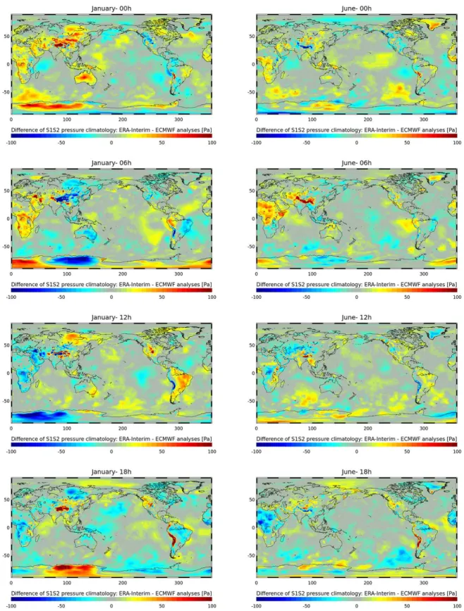
complemen-tary to the ocean tide correction, is based on Ponte and Ray (2002); it consists of removing S1 and S2 atmospheric pressure climatologies from the DAC forcing. Climatologies computed from 11 years of operational ECMWF data (1993– 2003; Carrere, 2005) are used for the operational DAC, but they are not coherent with the ERA-Interim data set. New monthly climatologies based on 18 years of ERA-Interim pressure data (1992–2009) have been computed and then re-moved from the DAC pressure forcing for the present study.
Figure 2 shows the difference between the new ERA-Interim pressure climatology and the one used for operational DAC: differences are lower than 100 Pa over oceans and can be stronger on land.
2.3.2 The new dynamic atmospheric correction derived from ERA-Interim
The ERA-Interim DAC correction (DAC_ERA) has been computed while forcing the MOG2D barotropic ocean model with the corrected ERA-Interim meteorological data de-scribed above. The interest of using an atmospheric model reanalysis is to improve the quality of DAC for the oldest years and thus improve the homogeneity of the correction for the entire altimetric period; improving homogeneity helps with estimating more accurate trends. The same postprocess-ing as the one used for the reference DAC (20-day filterpostprocess-ing) has been performed. The new correction has been computed for the 1991–2013 altimetric period.
2.4 The dry tropospheric correction
The propagation velocity of a radio pulse is slowed by dry gases and the quantity of water vapor in the Earth’s tropo-sphere. The dry gas contribution is nearly constant and pro-duces height errors of approximately−2.3 m. This effect can be modeled as the gases in the troposphere contribute to the index of refraction. In details, the refractive index depends on pressure and temperature. When hydrostatic equilibrium and the ideal gas law are assumed, the vertically integrated range delay is a function of the surface pressure only (Chel-ton, 2001). The dry meteorological tropospheric range cor-rection is defined by the following formula:
Dry_Tropo= −2.277·Patm(1+0.0026·cos(2·LAT)) (2)
where Patm is the surface atmospheric pressure in mbars,
LAT is the latitude, and Dry_Tropo is the dry tropospheric correction in millimeters.
As there is no straightforward way of measuring the nadir surface pressure from altimetry, it is determined from a global atmospheric model. The operational dry tropospheric correction (named DT_ECMWF hereafter) is based on the ECMWF operational analyses, which have a 6 h time resolu-tion (cf. AVISO, 2011).
2.4.1 Specific processing for S1 and S2 atmospheric tides
Concerning the dry tropospheric correction, the diurnal (S1) and semidiurnal (S2) atmospheric tides also demand spe-cific processing because they are not well sampled by the 6 h ECMWF pressure fields due to Nyquist theory.
The methodology chosen to correct the operational Dry_Tropo from S1 and S2 atmospheric tides, is based on Ponte and Ray (2002) to remove S1 and S2 atmospheric pressure climatology from the ECMWF pressure field, as de-scribed in the DAC Sect. 3.1.1. A second step consists of adding correct S1 and S2 atmospheric tides from a specific atmospheric tide model (Ray and Ponte, 2003).
2.4.2 The new dry tropospheric correction derived from ERA-Interim
The ERA-Interim dry tropospheric correction (DT_ERA) is based on the ERA-Interim atmospheric pressure (mean sea level pressure field), with a 6 h temporal resolution, and spe-cific S1 and S2 climatologies described in Sect. 3.1.1. The new correction is available for the 1991–2013 period. 2.5 Method of comparison
In order to compare the studied corrections and to estimate their impact on the accuracy of altimeter data, the first step consists of interpolating the grids of DAC and DT correc-tions on the satellites’ ground tracks bilinearly in space and time. Differences between ERA-Interim-based corrections and the operational ECMWF corrections can then be inves-tigated along track for each altimeter. The along-track inter-polated values also allow computing the altimeter SSH suc-cessively using each of the corrections, ERA-based or op-erational ones. The differences in the sea level contents are analyzed for different time and spatial scales. Notice that even the pressure-derived corrections solely depend on the state of the atmosphere, considering several altimeters allows studying different temporal periods: for example, TP, Jason-1, and Jason-2 are consecutive data sets. Moreover, as TP and ERS ground tracks have different orbit characteristics (cycle, heliosynchronous), using these two types of data allows for consideration of different aliasing problems.
The impact of DAC_ERA and DT_ERA is primarily es-timated for short temporal scales (time lags lower than 10 days), which are very significant for these corrections as they contain a large part of their variability (Vinogradova et al., 2007). Moreover, these short temporal scales are indirectly linked with climate scales since high temporal frequency er-rors increase the formal error estimation of larger temporal scale signals.
L. Carrere et al.: Major improvement of altimetry sea level estimations 829
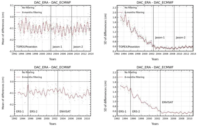
Figure 3.Temporal evolution of the global differences between DAC_ERA and the operational DAC seen by each altimeter mission: TP, Jason-1, and Jason-2 (top), and ERS-1, ERS-2, and Envisat (bottom) (mean and standard deviation in centimeters).
of each altimeter, successively using the studied correc-tion and the reference one. Crossover points with time lags shorter than 10 days within one cycle are selected in order to minimize the contribution of the ocean variability at each crossover location. The DAC is by essence a high-frequency correction as described in Sect. 3.1, with short temporal auto-correlation scales (Lamouroux, 2006; Mourre, 2004), and the DT is directly proportional to pressure field (cf. Sect. 3.2); thus, this diagnostic allows a good estimation of the impact of the DAC and the DT correction on the high-frequency part of the altimeter SSH, focusing on signals with periods below 10 days in the case of this crossover’s diagnostics.
The maps of the variance difference of SSH differences at crossover points successively using each altimetric com-ponent in the SSH calculation are first computed; they are computed on small boxes of 4◦×4◦and give information on
the temporal variance of the SSH differences. The long-term monitoring of SSH is estimated thanks to the calculation of global statistics for each altimeter cycle, all along the time span of each mission, and considering multi-mission con-catenated time series as described in Fig. 1; this gives infor-mation about the temporal evolution of the spatial variance of the SSH differences. For both diagnostics, the reduction of variance indicates a better internal consistency of sea level between ascending and descending passes within a 10-day window and thus characterizes a better SSH performance. SSH differences at crossovers focus on HF variability and
the spatial resolution of this diagnostic is limited due to the localization of crossovers.
To pursue the analysis further to the coast, we consider track observations instead of crossovers: the along-track SLA statistics are calculated from 1 Hz altimetric mea-surements. Although high-frequency signals are aliased in the lower-frequency band following the Nyquist theory ap-plication to each altimeter sampling, SLA time series con-tain the entire ocean variability spectrum. To investigate the impact of the new DAC near the coasts, the differences of SLA variances, computed by successively using both DAC corrections, can be plotted as a function of coastal distances between 0 and 100 km.
The analysis is finally focused on ocean long-term evolu-tion at global and regional scales, which is relevant for cli-mate studies. The global and regional MSL trends are com-puted for each altimetric mission considered here (from 1992 onwards), applying the MSL calculation method described on AVISO website:
http://www.aviso.altimetry.fr/en/data/products/
L. Carrere et al.: Major improvement of altimetry sea level estimations 831
Figure 4.Statistics of differences between DAC_ERA and the operational DAC seen by ERS-1, ERS-2, and Envisat altimeter missions (mean and standard deviation in centimeters).
and a least square method at each grid point. Trends are estimated for each SLA successively using the studied and the reference DAC and DT corrections. Notice that the trends of the altimetric missions can be very different one to the other due to the impact of the mission’s timespan on the trend estimation, with a longer timespan allowing a more accurate trend estimation. The error bar of the MSL trends’ estimation is about 0.5 mm yr−1(Ablain et al., 2015).
3 Analysis of the differences of atmospheric pressure-derived corrections
In this section, we analyze the differences between the refer-ence (ECMWF-based) and the studied (ERA-Interim-based)
atmospheric pressure-derived corrections, namely DAC and DT, at global and regional scales; a long-term analysis of these differences is also presented for the 20 years of altime-try data available.
3.1 The dynamic atmospheric correction
Figure 5.Temporal evolution of the differences between dry tropospheric ERA and the operational dry tropospheric correction seen by each altimeter missions series: TP, J1, J2 time series (top), and ERS-1, ERS-2, and Envisat time series (bottom) (mean and standard deviation in centimeters).
ERS-1, ERS-2, and Envisat missions, which cover the nearly entire altimetric period considered.
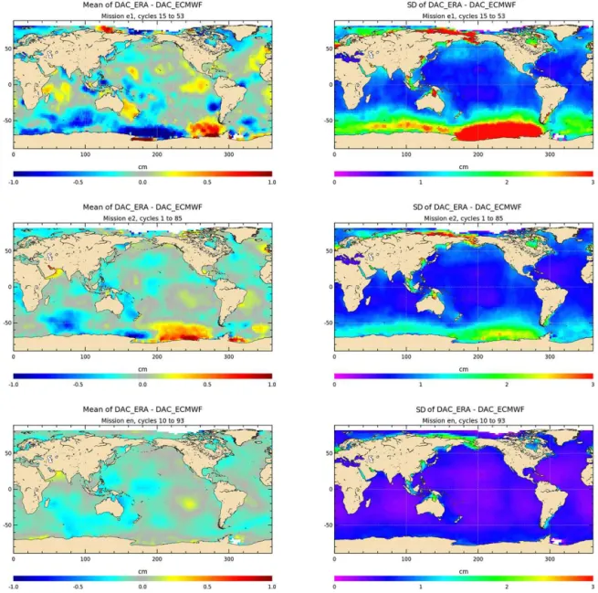
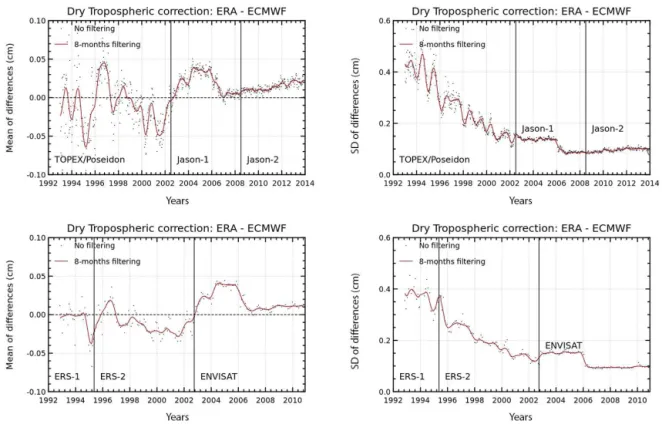
The mean difference between both corrections is about 1 mm, with annual variations below a few tenths of a mil-limeter for all missions. The standard deviation of the differ-ences clearly evolves with time, with strong differdiffer-ences for the first years of altimetry (up to 1.6–1.8 cm for ERS-1 and TP) which decrease until the year 2002 and then become sta-ble around 0.5 cm for Envisat, Jason-1, and Jason-2. A low annual signal is likely explained by the seasonal ice cover’s impact.
The maps of the differences also indicate stronger values for old altimeter missions: the mean of differences shows values up to 1 cm or even more in some large regions mainly located in southern high latitudes for 1, ERS-2, and in the Arctic and other ocean regions for ERS-1. As expected from the atmospheric pressure and wind high-frequency variability, the standard deviation of differences shows weak differences in the intertropical area (between latitudes 40◦S/40◦N) and strong differences of several
cen-timeters (over 3 cm) in southern high latitudes, in the Bering Strait, in the Arctic, and in some shallow water regions. The differences are stronger in the southern Pacific for the three old missions considered and significantly higher for the old-est one, ERS-1.
Concerning more recent missions such as Envisat, mean differences maps show some patterns with small differences below 0.4 cm, and standard deviation maps indicate values below 0.8 cm on most of the global ocean and up to 1.8–2 cm in a few shallow water regions. Those results confirm that both atmospheric models considered are very close in recent years, but some differences remain in shallow waters likely explained by the lower resolution of the reanalysis for this period.
3.2 The dry tropospheric correction
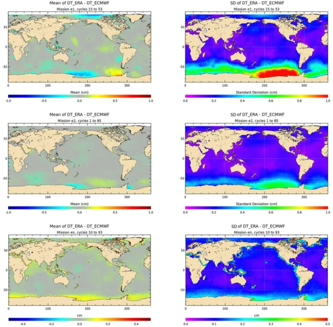
Figure 5 shows the monitoring of the global standard deviation and mean differences between DT_ERA and DT_ECMWF corrections during a 20-year period. Figure 6 shows the map of the differences between both corrections (mean and standard deviation) for the ERS-1, ERS-2, and Envisat missions.
L. Carrere et al.: Major improvement of altimetry sea level estimations 833
Figure 6.Maps of differences between DT_ERA and the ECMWF operational DT seen by altimeter missions ERS-1, ERS-2, and Envisat (mean and standard deviation in centimeters).
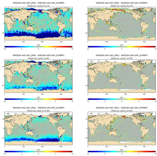
Figure 8.Maps of SSH variance differences at crossovers successively using the ERA-Interim and reference DAC solutions in the SSH calculation for ERS-1, ERS-2, and TP (on the left), and for Envisat, J1, and J2 (on the right) (cm2).
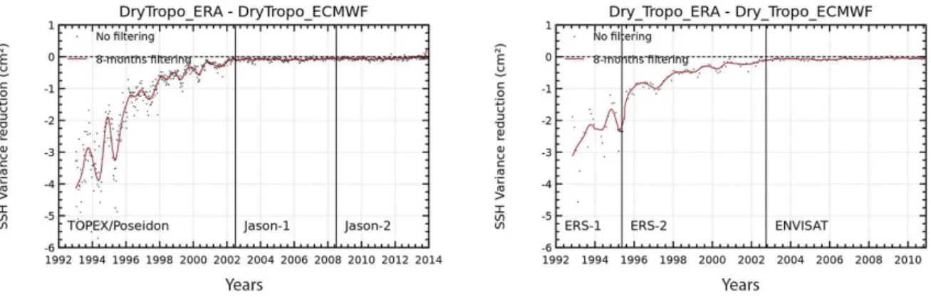
deviation of differences at the beginning of the year 2006; this is likely explained by the resolution change from N256 to N400 of the ECMWF native grid, and indicates that the DT correction is more affected than DAC by the meteorological model evolutions (cf. ECMWF system evolutions website).
The maps of the differences indicate also stronger values for the old missions – ERS-1 and ERS-2 – than for the more recent Envisat mission; the global mean differences are low for all missions (below 5 mm). Following the atmospheric pressure variability pattern, the variability of the difference is stronger in the southern high latitudes and reaches more than 1 cm for ERS-1 and up to 0.7 cm for ERS-2, and only 0.2 cm for Envisat. We also notice some small-scale oscilla-tions on Envisat maps which are explained by some errors occurring in the operational DT fields based on the Gaussian
grid of surface pressure (Gibbs oscillations) used since 2002 (Dibarboure, 2003).
4 Ocean short temporal scales
L. Carrere et al.: Major improvement of altimetry sea level estimations 835
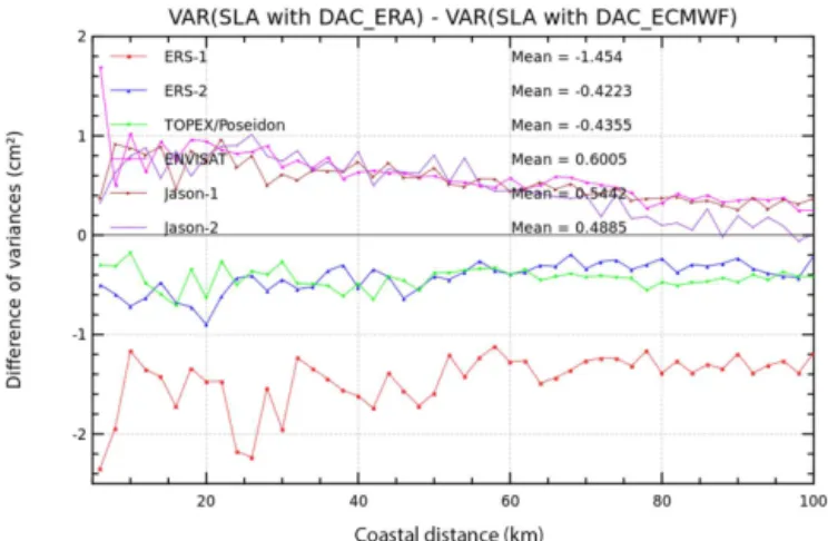
Figure 9. Difference of variance of SLA successively using the ERA-Interim and reference DAC solutions in the SSH calculation, for each altimeter, and as a function of distance to coast.
4.1 DAC
The impact of the new DAC_ERA on the SSH performance is first quantified by plotting the temporal evolution of SSH variance differences at crossovers successively using the dif-ferent DAC in the SSH calculation (cf. Fig. 7), respectively, for the TP/Jason-1/Jason-2 and the ERS-1/ERS-2/Envisat al-timeter time series. We note that DAC_ERA strongly reduces the SSH variance compared to the operational DAC on the first years of altimetry: the reduction reaches 5–12 cm2for the 1992–1996 period, and it corresponds to a mean diminu-tion of the along-track SSH error of 2–3 cm when using DAC_ERA, which is a very important result. Then this im-pact diminishes until 2002, but it still remains significant.
Concerning more recent missions (Jason-1, Jason-2, and Envisat), DAC_ERA and DAC_ECMWF have compara-ble results in terms of crossover variance reduction: dif-ferences remain between±1 cm2 on average during 2002–
2014. DAC_ERA tends to slightly raise the variance com-pared to ECMWF operational correction only from 2006 and onwards. The very close results of DAC_ERA and DAC_ECMWF in the recent altimeter period are remarkable and not expected since the operational ECMWF model has benefited from significant improvements over time. Evolu-tion of ECMWF operaEvolu-tional data set is linked to improved modeling, resolution, and data assimilation process: opera-tional database has a 0.5◦resolution until 2006, to be
com-pared to the 0.7◦of ERA-Interim; then the operational model
resolution changed to N400 (∼0.2◦) in January 2006, and to N640 in 2010 (cf. ECMWF evolutions website). Global ocean results suggest that modeling and data assimilation im-provements contained in ERA-Interim have a very important impact and overwhelm the lower resolution issue of ERA-Interim for most of the studied period, even until 2006. Only the last versions of the ECMWF operational model tend to
slightly improve DAC_ECMWF compared to DAC_ERA in the recent years.
To investigate regional patterns, the maps of SSH variance difference at crossovers successively using the DAC_ERA and the reference DAC, for each altimeter mission are plot-ted in Fig. 8: old missions (ERS-1, ERS-2, and TP) and the recent ones (Jason-1, Jason-2, and Envisat). Regionally, the improvement of sea level estimation is very significant using the DAC solutions derived from ERA-Interim for all old mis-sions tested (ERS-1, ERS-2, and TP): DAC_ERA allows the reduction of the residual variance at crossovers by more than 10 cm2in the Southern Ocean where the high-frequency dy-namic response of the ocean to atmospheric forcing is very important (Webb and de Cuevas 2002a, b, 2003; Carrere, 2003; Vinogradova and Ponte, 2007). The reduction is also significant in many shallow water regions like the Bering Strait, the Hudson Bay, the Patagonian Shelf, north Australia, the Yellow Sea, and the Arctic Ocean. In all those regions, DAC_ERA correction allows diminishing the along-track er-ror by more than 3 cm, compared to DAC_ECMWF, which is very significant. Those results show that the ERA-Interim re-analysis is much more accurate than the operational ECMWF model, which is used to compute the reference DAC, in the first decade of altimetry.
If considering the second decade of altimetry (Envisat, Jason-1, and Jason-2), both models of DAC have a similar impact in deep ocean regions but using DAC_ERA raises the SSH crossovers variance in some shallow water regions like the Bering Strait, the Arctic Ocean, the South China Sea, the Patagonian Shelf, or around Australia. This local vari-ance increase can be explained by the better resolution of the operational forcing in the recent years, which is an as-set to solving the short spatial scales characteristic of shal-low coastal areas; this increase is stronger for Envisat and Jason-2 which are the most recent altimeters studied here. The impact of DAC_ERA as a function of distance to coast for the global ocean is shown in Fig. 9, confirming previous results: DAC_ERA allows reducing the SLA variance near the coasts for old altimeter missions while it tends to raise it slightly when considering more recent missions.
4.2 Dry tropospheric correction
Figure 10.Temporal evolution of SSH variance differences at crossovers successively using the ERA-Interim and ECMWF operational DT corrections in the SSH calculation for TOPEX/Jason-1/Jason-2 series (on the left), and ERS-1/ERS-2/Envisat (on the right).
L. Carrere et al.: Major improvement of altimetry sea level estimations 837
Figure 12.Maps of MSL trend differences successively using the DAC derived from ERA-Interim and from ECMWF operational pressures fields (reference) for ERS-1, ERS-2, and TOPEX (on the left), for Envisat, Jason-1, and Jason-2 (on the right) (mm yr−1).
Table 2.Impact of ERA-Interim-based corrections (DAC_ERA and DT_ERA) on global MSL trends and the least square root estimation error (LSR) (mm yr−1).
Altimeter mission MSL trend using ECMWF Difference of MSL trend: Difference of MSL trend: corrections (reference) ECMWF – DAC_ERA ECMWF – DT_ERA
±LSR
ERS-1 6.34±0.62 0.07 0.01
ERS-2 2.66±0.15 0.01 −0.02
TP 3.12±0.03 −0.02 0.01
EN 2.28±0.18 −0.04 −0.03
J1 2.55±0.07 0 −0.02
Figure 13.Maps of MSL trend differences successively using the DT correction derived from ERA-Interim and from ECMWF operational pressures fields (reference) for ERS-1, ERS-2, and TOPEX (on the left), for Envisat, Jason-1, and Jason-2 (on the right) (mm yr−1).
this impact diminishes until it gives similar results to the operational DT_ECMWF for the 2002–2013 period. It is worth noting that the SSH variance reduction obtained with DT_ERA remains negative for the entire period, showing a slight improvement in the last decade; this result was not ex-pected.
The maps of SSH variance difference at crossovers suc-cessively using DT_ERA and DT_ECMWF (cf. Fig. 11) give information about the regional patterns of this improvement for each altimeter. The maximum variance reduction is lo-calized at high latitudes, where the variability of atmospheric pressure is at its maximum. The regional improvement of sea level estimation is very significant using the DT_ERA solu-tion for all old missions, ERS-1, ERS-2, and TP: the variance
gain is the strongest for ERS-1 and reaches more than 10 cm2 in the high latitudes. For ERS-2 and TP, the variance gain is a bit smaller but remains significant in the Southern Ocean.
L. Carrere et al.: Major improvement of altimetry sea level estimations 839 5 Ocean long-term climate signals
The impact of using the new ERA-Interim-derived atmo-spheric corrections (DAC_ERA and DT_ERA) instead of the operational correction is analyzed in terms of long-term trends of the altimeter SLA. Operational ECMWF analyses are known to contain drifts due to the evolution of the oper-ational model upon time (change of computoper-ational methods and in the data assimilation system; Thorne and Vose, 2010), which can impact the MSL trend estimations (Ablain et al., 2009). As meteorological reanalyses ensure greater homo-geneity of the database over time, they are thus more suit-able for long-term signal estimations as already discussed by Ablain et al. (2009) and Legeais et al. (2014). Moreover, re-duced high-frequency errors, thanks to the better quality of the reanalysis as described in previous sections, will decrease the formal error estimation of the long-term signals such as the MSL trend. MSL trends at global and regional scales are investigated as described in Sect. 2.3. Particularly as the dif-ference between ECMWF and ERA-Interim-based correc-tions shows large spatial patterns of strong variability, the regional MSL trends may be significantly affected by the use of the pressure-derived corrections based on ERA-Interim.
Global analysis shows that the new ERA-Interim-based solutions have a very small impact on the estimation of the global MSL trends of different altimeter missions considered in the study: Table 2 indicates that differences of trends are smaller than 0.07 mm yr−1, which is 1 order of magnitude
lower than the global MSL trend uncertainty: 0.5 mm yr−1
(Ablain et al., 2015). Even meteorological models can have instabilities or jumps due to model evolutions, this weak im-pact on global trends could be expected as the mean pres-sure is removed to perform the IB and to force the barotropic model, and the DAC is computed with an instantaneous zero mean. As seen in Fig. 5, the DT is more affected by meteoro-logical model evolutions as it depends on the pressure field, but results indicate that the impact on MSL trend is negligi-ble at a global scale.
Notice that the trend differences observed between each mission are not significant, as they are mostly explained by the different lengths of the temporal series available.
The impact of using ERA-Interim-based corrections on the regional MSL trends’ estimation is analyzed in terms of spa-tial distribution of the MSL trends for each mission consid-ered in the study (cf. Figs. 12 and 13). Although no impact is detected on the global MSL trend, using DAC_ERA cor-rection instead of DAC_ECMWF has a significant impact on the estimation of regional trends. Considerable trend differ-ences are displayed for the oldest missions; differdiffer-ences are located nearly everywhere on the global ocean for ERS-1 (±7 mm yr−1) and are likely explained by the strong differ-ences between DAC_ERA and DAC_ECMWF for this pe-riod, but also by the short time span of the ERS-1 temporal series, which makes the MSL trends’ estimation less accurate and less stable. MSL trends differences are mostly located
in the southern high latitudes for ERS-2 (±2.5 mm yr−1)
and TP (±1.5 mm yr−1), which correspond to the regions
where the differences between the DAC solutions themselves are the greatest and also where the SSH variance reduction is strong. Concerning more recent missions, the impact of DAC_ERA on regional MSL trends’ estimation is smaller than for old missions, but it is still not negligible: differ-ences locally reach 1–1.5 mm yr−1for Envisat, Jason-1, and
Jason-2. The impact of DAC_ERA on the estimation of re-gional trends is likely explained by the fact that DAC_ERA strongly reduces the high-frequency variability locally as dis-cussed in previous sections, and thus the formal error of the least square adjustment of the MSL trends is also reduced; this impact is all the more important because the regional trends are more affected by the oceanic variability and an-nual/semiannual signals than global trends.
Using the new DT_ERA correction instead of the DT_ECMWF has a weak impact on the regional MSL trends, as seen in Fig. 13: differences are lower than 0.3 mm yr−1 on the global ocean for most of missions. Differences are stronger for the ERS-1 mission, reaching 0.5 mm yr−1 or even a bit more on nearly the entire ocean, but these stronger values are likely mainly due to the shorter time series avail-able for this mission.
The different diagnostics presented here point out some differences for long-term regional trends’ estimation, when using the ERA-based corrections instead of operational cor-rections, but they do not demonstrate which trend is the most realistic. Comparisons with in situ measurements (Valladeau et al., 2012) as well as tide gauges or temperature and salin-ity profiles do not allow obtaining relevant results mainly due to the errors of the methods. However, as the DAC_ERA and DT_ERA induce strong improvements when considering short temporal scales (cf. Sect. 4), and because these high fre-quencies are related to lower frefre-quencies through the aliasing phenomena and contribute to the formal error estimation of longer timescale signals, we can assume that the DAC_ERA and the DT_ERA corrections have a positive impact on re-gional MSL trends’ estimation.
6 Discussion and conclusions
New DAC and DT corrections derived from the ERA-Interim reanalysis have been computed for the entire altimetric pe-riod. These corrections have been extensively compared to the operational DAC and DT solutions using long time series of six altimeter missions: ERS-1, ERS-2, TP, Envisat, Jason-1, and Jason-2.
a significant improvement in shallow waters where the ocean has a strong dynamic response to atmospheric forcing at high frequencies. Using the new DAC_ ERA correction induces a diminution of the along-track SSH error of about 1–2.4 cm globally and even more than 3 cm at high latitudes and in shallow waters. Although the DT correction has a lower vari-ability compared to the DAC, using the new DT_ERA al-lows reduction of the along-track SSH error by 1–2 cm on the global ocean and by more than 3 cm at high latitudes.
Unexpectedly in the three recent missions studied (En-visat, Jason-1, and Jason-2), ERA-based corrections show similar performances to the operational corrections although the meteorological reanalysis has a larger spatial resolu-tion than the ECMWF operaresolu-tional analyses. Moreover, DT_ ERA remains better than DT_ECMWF on the global ocean even in the most recent mission, Jason-2. DAC_ERA and DAC_ECMWF have comparable results in the deep ocean, but DAC_ERA tends to raise the residual crossovers vari-ance in some shallow water regions, where the finer resolu-tion of operaresolu-tional forcing seems more appropriated to solve the small spatial scales characteristic of shallow and coastal ocean dynamic.
Concerning long temporal scales relative to climate stud-ies, the present analysis shows that the ERA-based correc-tions do not have a significant impact on the global MSL trends. Using DT_ERA does not impact the regional MSL trends either. Using DAC_ERA has a strong effect on long-term regional trends’ estimation, with trend differences of several millimeters per year locally.
As the DAC_ERA induces a strong improvement when considering short temporal scales, and because these high frequencies are related to lower frequencies through the aliasing phenomena and contribute to the formal error of the MSL trends’ estimation, we can assume that the DAC_ERA has a positive impact on regional MSL trends’ estimation.
The results presented here allow recommending the use of DAC_ ERA in the first altimetry decade for ERS-1, ERS-2, and TP missions. For more recent missions, DAC_ERA can also be used at least for long-term signals’ estimation to get rid of any discontinuity between both DAC corrections, but at the cost of a slightly raised variance in some shallow water regions. Indeed, if using a combination of DAC_ ERA and operational DAC, the continuity between both DAC solutions at regional scales will need to be checked at least for long-term studies.
The dry tropospheric correction derived from ERA-Interim pressure field is also of great interest for all appli-cations, and this correction can be used for all altimeter mis-sions even the most recent one studied here, Jason-2.
Given the results of the present study, the DAC_ERA and the DT_ERA time series are still being completed in delayed time with a few months’ delay. These ERA-based corrections are used in several projects and products like REAPER (2014), CCI-phase-2 project (Ablain et al., 2015), SALP (SSALTO/DUACS, 2015), FES2012 and FES2014
tidal models (Carrere et al., 2012, 2014), and the Jason-1 re-processing project (Jason-1 products handbook, 2015).
As the ERA-Interim meteorological product has a coarse spatial resolution compared to the operational database in re-cent years, a perspective of this work will be to test a new atmospheric climatology with a finer spatial grid; this would likely help improving the results presented here in shallow waters and also in the southern deep ocean regions where the ocean response to meteorological forcing is enhanced for to-pography patterns.
7 Data availability
The altimeter AVISO SSALTO/DUACS real-time sea surface height measurements are available at http://www.aviso.altimetry.fr/en/data/products/ sea-surface-height-products/global.html. The climate-oriented altimeter sea level anomalies from the ESA climate change initiative project are accessible by request at [email protected] and details are provided at http://www.esa-sealevel-cci.org.
Acknowledgements. This work has been performed within the framework of the ESA Climate Change Initiative (CCI) and the SALP (CNES) projects. We thank Paul Poli from ECMWF for the elements of discussion he gave us on the ERA-Interim reanalysis, and Lionel Zawadzki from CLS for his help on the processings.
Edited by: A. Sterl
References
Ablain, M., Cazenave, A., Valladeau, G., and Guinehut, S.: A new assessment of the error budget of global mean sea level rate esti-mated by satellite altimetry over 1993–2008, Ocean Sci., 5, 193– 201, doi:10.5194/os-5-193-2009, 2009.
Ablain, M., Cazenave, A., Larnicol, G., Balmaseda, M., Cipollini, P., Faugère, Y., Fernandes, M. J., Henry, O., Johannessen, J. A., Knudsen, P., Andersen, O., Legeais, J., Meyssignac, B., Picot, N., Roca, M., Rudenko, S., Scharffenberg, M. G., Stammer, D., Timms, G., and Benveniste, J.: Improved sea level record over the satellite altimetry era (1993–2010) from the Climate Change Initiative project, Ocean Sci., 11, 67–82, doi:10.5194/os-11-67-2015, 2015.
AVISO: OSTM/Jason-2 products handbook, SALP-MU-M-OP-15815-CN, Edn. 1.8, http://www.aviso.oceanobs.com/fileadmin/ documents/data/tools/hdbk_j2.pdf (last access: 13 May 2015), 2011.
Carrere, L.: Etude et modélisation de la réponse haute fréquence de l’océan global aux forçages météorologiques, Toulouse, univer-sité Toulouse III – Paul Sabatier, 2003.
Carrere, L.: Rapport d’étude CNES/CLS, reference CLS-DOS-NT-05-007, 2005.
L. Carrere et al.: Major improvement of altimetry sea level estimations 841
comparisons with observations, Geophys. Res. Lett., 30, 1275, doi:10.1029/2002GL016473, 2003.
Carrere, L., Lefèvre, F., Briol, F., Dorandeu, J., Roblou, L, Jeansou, E., Jan, G., and Lyard, F.: New improvements on the Dynamic Atmospheric Corrections, OSTST, Tides/HF Aliases splinter ses-sion, Hobart, Tasmania, 2007.
Carrere, L., Faugère, Y., Dibarboure, D., Bronner, E., and Ponte, R.: Improving the Dynamic Atmospheric Correction for altime-try – impact of 3-hours meteorological fields, OSTST poster presentation, http://www.aviso.altimetry.fr/fr/coin-utilisateur/ equipes-scientifiques/ostst-swt-science-team.html (last access: 23 June 2016), 2010.
Carrere, L., Lyard, F., Cancet, M., Guillot, A., Faugère, Y., and Roblou, L.: FES 2012: a new global tidal model taking advan-tage of nearly 20 years of altimetry, 20 years of progress in radar altimetry symposium, Venice, 2012.
Carrere, L., Lyard, F., Cancet, M., Guillot, A., Faugère, Y., and Pi-cot, N.: FES 2014: a new tidal model on global ocean, OSTST, Tides/HF session, Constance, 2014.
Cazenave, A., Dieng, H., Meyssignac, B., von Schuckmann, K., Decharme, B., and Berthier, E., The rate of sea level rise, Nature Climate Change, 4, 358–361, doi:10.1038/NCLIMATE2159, 2014.
Chelton, D. B., Ries, J. C., Haines, B. J., Fu, L. L., and Callahan, P. S.: Satellite Altimetry, Satellite Altimetry and Earth Sciences, edited by: Fu, L. L. and Cazenave, A., 1–131, 2001.
Couhert, A., Cerri, L., Legeais, J.-F., Ablain, M., Zelensky, N., Haines, B., Lemoine, F., Bertiger, W., Desai, S., and Ot-ten, M.: Towards the 1 mm/y Stability of the Radial Or-bit Error at Regional Scales, Adv. Space Res., 55, 2–23, doi:10.1016/j.asr.2014.06.041, 2014.
Dee, D. P., Uppala, S. M., Simmons, A. J., Berrisford, P., Poli, P., Kobayashi, S., Andrae, U., Balmaseda, M. A., Balsamo, G., Bauer, P., Bechtold, P., Beljaars, A. C. M., van de Berg, L., Bid-lot, J., Bormann, N., Delsol, C., Dragani, R., Fuentes, M., Geer, A. J., Haimberger, L., Healy, S. B., Hersbach, H., Hólm, E. V., Isaksen, L., Kållberg, P., Köhler, M., Matricardi, M., McNally, A. P., Monge-Sanz, B. M., Morcrette, J.-J., Park, B.-K., Peubey, C., de Rosnay, P., Tavolato, C., Thépaut, J.-N., and Vitart, F.: The ERA-Interim reanalysis: configuration and performance of the data assimilation system., Q. J. Roy. Meteor. Soc., 137, 553–597, doi:10.1002/qj.828, 2011.
Dibarboure, G.: Comparaison des Corrections Météo Gaussi-ennes et CartésiGaussi-ennes utilisées dans SSALTO/DUACS, report CLS/CNES, CLS-DOS-NT-03-915, 2003.
ECMWF: system evolutions: http://www.ecmwf.int/en/forecasts/ documentation-and-support/changes-ecmwf-model, last access: March 2016.
Greenberg, D., Dupont, F., Lyard, F., Lynch, D., and Werner, F.: Resolution issues in numerical models of oceanic and coastal cir-culation, Cont. Shelf Res., 27, 1317–1343, 2007.
Hernandez, F. and Schaeffer, P.: The CLS01 Mean Sea Surface: A validation with the GSFC00.1 surface, CLS report, 2001. Jason-1 products handbook: http://www.aviso.altimetry.fr/
fileadmin/documents/data/tools/hdbk_j1_gdr.pdf (last access: 4 April 2016), 2015.
Lamouroux, J.: Erreur de prévision d’un modèle océanique barotrope du Golfe de Gascogne en réponse aux incertitudes sur les forçages atmosphériques. Caractérisation et utilisation dans
un schéma d’assimilation de données à ordre réduit, PhD, Uni-versity Paul Sabatier, Toulouse, 2006.
Lamouroux, J., De Mey, P., Lyard, F., and Jeansou, E.: Study of the MOG2D model sensitivity to high frequency atmospheric forc-ing in the Bay of Biscay, and assimilation of altimetric and tide-gauge observations in order to correct the model for the deficien-cies of the atmospheric forcing fields, Mercator Ocean Quarterly Newsletter, 23, 5–14, 2006.
Legeais, J.-F., Ablain, M., and Thao, S.: Evaluation of wet tropo-sphere path delays from atmospheric reanalyses and radiometers and their impact on the altimeter sea level, Ocean Sci., 10, 893– 905, doi:10.5194/os-10-893-2014, 2014.
Mathers, E. L. and Woodworth, P. L.: Departure from the local in-verse barometer model observed in altimeter and tide gauge data and in a global barotropic numerical model, J. Geophys. Res., 106, 6957–6972, 2001.
Mourre, B.: Etude de configuration d’une constellation de satel-lites altimétriques pour l’observation de la dynamique océanique côtière, PhD, University Paul Sabatier, Toulouse, 2004. Ponte, R. M. and Gaspar, P.: Regional analysis of the inverted
barometer effect over the global ocean using Topex/Poseidon data and model results, J. Geophys. Res., 104, 15587–15601, 1999.
Ponte, R. M. and Ray, R. D.: Atmospheric Pressure Cor-rections in Geodesy and Oceanography: a strategy for handling air tides, Geophys. Res. Lett., 29, 2253–2256, doi:10.1029/2002GL016340, 2002.
Ray, R.: A global ocean tide model from Topex/Poseidon altimetry: GOT99.2, NASA Tech Memo 209478, 58 pp., 1999.
Ray, R. D. and Ponte, R. M.: Barometric tides from ECMWF operational analyses, Ann. Geophys., 21, 1897–1910, doi:10.5194/angeo-21-1897-2003, 2003.
REAPER: Product Handbook for ERS Altimetry Reprocessed Products, https://earth.esa.int/documents/10174/1511090/ Reaper-Product-Handbook-3.1.pdf (last access: 21 August 2014), 2014.
SSALTO/DUACS: User Handbook: (M)SLA and (M)ADT Near-Real Time and Delayed Time Products, http: //www.aviso.altimetry.fr/en/data/product-information/
aviso-user-handbooks.html (last access: 30 June 2015), v4.4, 2015.
Stammer, D., Wunsch, C., and Ponte, R. M.: De-aliasing of global high frequency barotropic motions in altimeter observations, Geophys. Res. Lett., 27, 1175–1178, 2000.
Thorne, P. W. and Vose, R. S.: Reanalyses Suitable for Character-izing Long-Term Trends, B. Am. Meteorol. Soc., 91, 353–361, doi:10.1175/2009BAMS2858.1, 2010.
Valladeau, G., Legeais, J.-F., Ablain, M., Guinehut, S., and Picot, N.: Comparing Altimetry with Tide Gauges and Argo profiling floats for data quality assessment and Mean Sea Level studies, Mar. Geod., 35, suppl. 1, 42–60, doi:10.1080/01490419.2012.718226, 2012.
Vinogradova, N. T., Ponte, R. M., and Stammer, D.: Relation be-tween sea level and bottom pressure and the vertical depen-dence of oceanic variability, Geophys. Res. Lett., 34, L03608, doi:10.1029/2006GL028588, 2007.
Webb, D. J. and de Cuevas, B. A.: An ocean resonance in the In-dian sector of the Southern ocean, Geophys. Res. Lett., 29, 1664– 1667, doi:10.1029/2002GL015270, 2002b.
Webb, D. J. and de Cuevas, B. A.: The region of large sea sur-face height variability in the southeast Pacific Ocean, J. Phys. Oceanogr., 33, 1044–1056, 2003.
Willebrand, J., Philander, S., and Pacanowski, R.: The oceanic response to large-scale atmospheric disturbances, J. Phys. Oceanogr., 10, 411–429, 1980.