FORECASTING ANTARCTIC SEA ICE CONCENTRATIONS USING RESULTS OF TEMPORAL MIXTURE ANALYSIS

(1)

FORECASTING ANTARCTIC SEA ICE CONCENTRATIONS USING RESULTS OF

TEMPORAL MIXTURE ANALYSIS

Junhwa Chi, Hyun-Cheol Kim

Department of Polar Remote Sensing, Korea Polar Research Institute, Incheon, Korea - (jhchi, kimhc)@kopri.re.kr

Commission VIII, WG VIII/6

KEY WORDS: Temporal mixture analysis, times series model, sea ice concentration, AR model

ABSTRACT:

Sea ice concentration (SIC) data acquired by passive microwave sensors at daily temporal frequencies over extended areas provide seasonal characteristics of sea ice dynamics and play a key role as an indicator of global climate trends; however, it is typically challenging to study long-term time series. Of the various advanced remote sensing techniques that address this issue, temporal mixture analysis (TMA) methods are often used to investigate the temporal characteristics of environmental factors, including SICs in the case of the present study. This study aims to forecast daily SICs for one year using a combination of TMA and time series modeling in two stages. First, we identify temporally meaningful sea ice signatures, referred to as temporal endmembers, using machine learning algorithms, and then we decompose each pixel into a linear combination of temporal endmembers. Using these corresponding fractional abundances of endmembers, we apply a autoregressive model that generally fits all Antarctic SIC data for 1979 to 2013 to forecast SIC values for 2014. We compare our results using the proposed approach based on daily SIC data reconstructed from real fractional abundances derived from a pixel unmixing method and temporal endmember signatures. The proposed method successfully forecasts new fractional abundance values, and the resulting images are qualitatively and quantitatively similar to the reference data.

1. INTRODUCTION

Sea ice dynamics play an important role in climate change and global warming studies by revealing high latitude temperature trends. Sea ice in the Arctic has exhibited a long-term negative trend while sea ice in the Antarctic has been expanding for decades (Parkinson et al., 2012). Sea ice concentration (SIC) is typically estimated using passive microwave data because of the daily revisit cycle, the relatively low sensitivity to atmospheric water content and clouds, and the large contrast in emissivity between open water and sea ice (Comiso et al., 1997, Ivanova et al., 2014).

Among the various analysis techniques designed to utilize time series remotely sensed data, temporal mixture analysis (TMA), which is an extension of the spectral mixture analysis (SMA) of multispectral or hyperspectral remote sensing images, is receiving increased attention for use in summarizing and analyzing long-term time series data. TMA provides seasonal characteristics of univariate information such as SIC as well as a unique summary of long-term time series (Piwowar et al., 1998, Chi et al., 2016). In addition to sea ice studies, TMA has been applied to various applications in agriculture and urban studies

A recent study conducted by Chi et al. (2016) analyzed long-term Antarctic daily SICs using machine learning-based TMA techniques. The authors examined hypertemporal SIC data without incorporating prior knowledge of seasonal sea ice signatures. Representative temporal endmembers were extracted from 36 years of daily SIC data and were then used to compute corresponding fractional abundances of each temporal endmember component. In this study, we propose a novel approach of forecasting daily SIC for the present year (2014) using TMA results derived from previous years (1979-2013) reported in Chi et al. (2016) and using time series analysis models.

2. METHODOLOGY

TMA can be applied to any univariate data stacked in the time domain. In this study, we examine 36 years of daily Antarctic SIC data acquired from 1979 to 2014, provided by the NSIDC (National Snow and Ice Data Center), based on the assumption that the data quality is guaranteed at a global scale. The data were generated from a passive microwave sensor SMMR (Scanning Multi-channel Microwave Radiometer) and SSMIS (Special Sensor Microwave Imager/Sounder) at a 25 km spatial resolution in the polar stereographic projection. To extract consistent SICs from different sensors, the NASA Team algorithm was used (Cavalieri et al. 1996).

2.1 Temporal mixture analysis

SMA has been extensively investigated and successfully applied in the development of new algorithms and multispectral and hyperspectral remote sensing applications, but few studies have been carried out on TMA algorithms and applications, as TMA research is still in its infancy and it is difficult to acquire high-frequency temporal images. Because TMA is algebraically identical to SMA and shares its main concepts, assuming that the linear model is a good approximation, two general stages similar to those of SMA are used to address the temporal mixing problems. The first stage involves identifying temporally meaningful and unique signatures of pure substances, which are referred to as temporal endmembers, using machine-learning techniques for quantitative and automatic selection. The second step involves decomposing each pixel in the time series images into a collection of temporal endmembers using a linear combination (Keshava and Mustard 2002).

Similar to hyperspectral data but for a different domain, most pixels in time series data are often decomposited by several representative temporal substances. Over the last decade, various algorithms have been developed and used for the automatic

The International Archives of the Photogrammetry, Remote Sensing and Spatial Information Sciences, Volume XLI-B8, 2016 XXIII ISPRS Congress, 12–19 July 2016, Prague, Czech Republic

This contribution has been peer-reviewed.

(2)

identification of spectral endmembers in SMA. Because Winter’s N-FINDR (Winter 1999), which uses the concept of convexity of geometry, has been one of the most successfully and widely applied techniques for automatically determining endmembers, we used this approach to automatically extract temporal endmembers. This algorithm searches through a set of pixels with the largest possible volume by inflating a simplex.

Assuming that the value of a mixed pixel is a linear combination of the values for endmember components, linear unmixing is the simplest and most widely used method for mixed pixel decomposition (Keshava and Mustard 2002). Each temporal pixel vector in the original image can be modeled using the following expression:

�"= �",&�& (

&)*

+ �" (1)

where � = daily SIC trajectory of SIC time series � = temporal endmember vector

� = number of temporal endmembers

� = fractional abundance of endmember vector � = noise vector

The least squares solution to computing fractional abundances by minimizing the pixel reconstruction error is as follows:

�",&= (�1�)3*�1�" (2)

where � = set of temporal endmembers

2.2 Time series analysis

The time series model (TSM) is a dynamic research area that has received attention over the last few decades and is a powerful tool for conducting temporal analyses. The primary goal of the TSM is to examine past observations of time series and to develop an appropriate model that describes the inherent structures of data. The model is then used to predict future values of time series based on the past (Hipel et al., 1994).

Various types of TSMs are used in a variety of practical applications. In this study on Antarctic SIC forecasting using TMA results, AR (AutoRegressive) models that relate current series values to past values and prediction errors are considered. AR models specify that the output variable depends linearly on its previous values and on a stochastic (i.e., imperfectly predictable) term (Box et al., 1994). Thus, the model is a special case of the more general ARMA (AutoRegressive Moving Average) models, which have promised reasonable outcomes in forecasting environmental time series relative to competing models (Hipel et al., 1994, Piwowar et al., 2010).

If we wish to predict the present value using p previous measurements, then the AR model can be mathematically written as follows:

�5= �*�53*+ �7�537+ ⋯ + �9�539+ �5 (3)

where � = parameters of AR model �₅= observation at time t � = white noise

The TSM of fractional abundances of corresponding temporal endmembers is produced by AR models and is inherently multivariate. One of the temporal endmembers used to predict employs past and present values of every other temporal endmember. The general multivariate form of the AR(p) model when the fractional abundances (�5, �5, �5) of three temporal endmembers are employed is as follows:

�5= �**,"�53" 9

")*

+ �*7,"�53" 9

")*

+ �*=,"�53" 9

")*

+ �*,5

�₅= �_7*,"�_53" 9

")*

+ �_77,"�_53" 9

")*

+ �_7=,"�_53" 9

")*

+ �_7,5 (4)

�5= �=*,"�53" 9

")*

+ �=7,"�53" 9

")*

+ �==,"�53" 9

")*

+ �=,5

3. EXPERIMENTAL RESULTS

The experiments in this study were conducted in two phases: 1) temporal mixture analysis and 2) time series analysis. The first phase involved computing time series fractional abundances of the representative temporal endmembers for 36 years. The results of the first stage were used to train time series models and to evaluate the model’s accuracy for the second stage. Each stage involved several steps, and more details are listed in the following subsections.

3.1 Temporal mixture analysis

The TMA stage is identical to the experimental part of the previous study (Chi et al., 2016) and is composed of three steps. To determine the number of temporal endmembers without prior knowledge, we first used the Harsanyi-Farrand-Chang (HFC) virtual dimensionality algorithm, which computes the sample correlation and covariance matrices and then determines the difference between the corresponding eigenvalues (Harsanyi et al., 1993). As there are numerous anomalous SIC pixels in daily SIC data acquired from 1979 to 2014 due to sensor and processing errors, the daily time series were smoothed by removing outliers using neighboring pixels and the moving average of the previous and following days. Additionally, because data from 1979 to 1987 were acquired every other day, linear interpolation was applied to generate consistent daily time series throughout the time period. Therefore, the number of potential and representative temporal endmembers was determined to be 9. Then, the N-FINDR algorithm was used to identify the 9 representative temporal endmembers showing the maximum variation in SIC throughout the year, as shown in Figure 1. Subsequently, the spatial distributions of the corresponding fractional abundances in 2014 associated with the temporal endmembers were generated, as shown in Figure 2. For detailed information on the temporal mixture analysis stage and experimental results, see Chi et al. (2016).

3.2 Time series analysis

To adequately apply AR models to image data, the order of the models should be determined for each time series. Our temporal image data acquired at a single time instance include 82,907 valid pixels (i.e., 25 km Antarctic SIC data include 332 x 316 pixels, but pixels for the Antarctic continent are excluded). Thus, 82,907

(3)

individual AR models are needed to properly fit all of the Antarctic SIC data. As the objective of this study is to automatically forecast future SIC using time series analysis approaches, individually and manually fitting models to the 82,907 pixels is very inefficient. In this study, we assume that most of the Antarctic SIC for 36 years could be fitted with AR models of the same degree and that the AR(1) model is appropriate for overall use.

3.3 Experimental results

Based on the assumption presented above, fractional abundances for 2014 were estimated using single AR(1) models trained by the entire time series of 35-year fractional abundances for 1979 to 2013 using the TMA method. Using forecasted abundances and temporal endmember signals derived from the endmember identification step, daily 365 SIC images for 2014 can be reconstructed via the inverse process of pixel unmixing. As discussed in Chi et al. (2016), TMA results can typically be tested using pixel reconstruction errors when reference data for temporal sea ice endmembers are not available. Thus, the root mean square error (RMSE) was used to provide an overall ‘pixel-by-pixel’ difference between the original and reconstructed images.

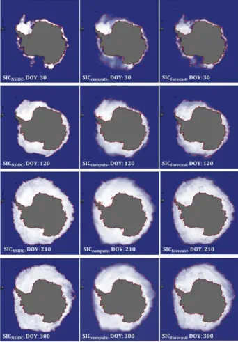
Figure 3 compares the original 2014 NSIDC SIC data SICABCDE for the selected days (day of year (DOY): 30, 120, 210, 300) with 1) reconstruction images using fractional abundances computed

via the pixel unmixing approach SIC_FGHIJKL proposed in Chi et al. (2016) and 2) reconstruction images based on forecasted fractional abundances of the single AR(1) model SICMGNLFOPK proposed in the present study. Red borders in each image denote sea ice extents (SIEs) where the regions of interest present SIC values of at least 15%. As discussed in Chi et al. (2016), the reconstructed SIC images (SICFGHIJKL, SICMGNLFOPK) did not typically capture detailed levels of variability in local areas and produced smoother SIC estimates. However, both concentrations and extents generally showed good visual agreement with the original images, as shown in Figure 3. Overall, the RMSE values

of SIC_FGHIJKL (8.5%) are statistically more accurate than those of

SICMGNLFOPK (12.9%). Although SICMGNLFOPK visually appears to

capture higher levels of local variability than SICFGHIJKL in certain regions, SIC_MGNLFOPK presents relatively low levels of statistical fidelity with SICABCDE for some regions that may be associated with the AR(1) model for rejected areas. In the SIE comparisons shown in Figure 3, extents based on forecasted fractional abundances (SIEMGNLFOPK) typically show higher levels of visual agreement with the original extents (SIEABCDE) than SIEs that use real fractions (SIEFGHIJKL). Daily averages of summed areas for all grid cells in SIE_MGNLFOPK were statistically very close to SIEABCDE (2.5% overestimated), whereas

SIEFGHIJKL was overestimated by approximately 15%. Therefore,

the proposed forecasting method captured higher levels of visual agreement with the original images and defined more accurate sea ice boundaries than the images reconstructed via pixel unmixing.

Figure 3. Extracted temporal endmembers

Figure 2. Fractional abundance maps for 2014

Figure 1. Daily SIC comparisons between the original and reconstructed images

(4)

4. CONCLUSIONS

In this study, fractional abundances for the past 35 years computed using the TMA approach were incorporated with AR(1) models in an effort to forecast new fractional abundances for the present year. The forecasted fractional abundances were used to compute reconstructed images using representative temporal endmembers identified using TMA method. The proposed results delivered results comparable with real values in terms of overall RMSE accuracy levels and visual agreement. SIEs derived from reconstructed SIC images showed better accuracy outcomes than the reconstruction SICs based on fractional values of pixel unmixing.

ACKNOWLEDGEMENTS

This study was supported by the Korea Polar Research Institute [grant number PE16040].

REFERENCES

Box, G.E., Jenkins, G.M., Reinsel, G.C., and Ljung, G.M., 2015. Time series analysis: forecasting and control. John Wiley & Sons.

Cavalieri, D.J., Parkinson, C.L., Gloersen, P., and Zwally, H., 1996. Sea Ice Concentrations From Nimbus-7 SSMR and DMSP SSM/I-SSMIS Passive Microwave Data, National Snow and Ice Data Center. Boulder, CO, USA.

Chi, J., Kim, H.-C., and Kang, S.-H., 2016. Machine learning-based temporal mixture analysis of hypertemporal Antarctic sea ice data. Remote Sensing Letters, 7(2), pp.190–199.

Comiso, J.C., Cavalieri, D.J., Parkinson, C.L., and Gloersen, P., 1997. Passive microwave algorithms for sea ice concentration: A comparison of two techniques. Remote Sensing of Environment, 60(3), pp.357–384.

Harsanyi, J.C., Farrand, W.H., and Chang, C.-I., 1993. Determining the Number and Identity of Spectral Endmembers: An Integrated Approach Using Neyman-Pearson Eigen-Thresholding and Iterative Constrained RMS Error Minimization. In: The Thematic Conference on Geologic Remote Sensing, San Antonio, TX, USA.

Hipel, K.W., and McLeod, A. I., 1994. Time series modelling of water resources and environmental systems (Vol. 45). Elsevier.

Ivanova, N., and Johannessen, O.M., 2014. Retrieval of Arctic sea ice parameters by satellite passive microwave sensors: A comparison of eleven sea ice concentration algorithms. IEEE Transactions on Geoscience and Remote Sensing, 52(11), pp.7233-7246.

Keshava, N., and Mustard, J.F., 2002. Spectral unmixing. IEEE Signal Processing Magazine, 19(1), pp.44–57.

Parkinson, C.L., and Cavalieri, D.J., 2012. Antarctic sea ice variability and trends, 1979–2010. The Cryosphere, 6(4), pp. 871-880.

Piwowar, J.M., and Ledrew, E.F., 2010. ARMA time series modelling of remote sensing imagery: A new approach for climate change studies. International Journal of Remote Sensing, 23(24), pp.5225–5248.

Piwowar, J.M., Peddle, D.R., and Ledrew, E.F., 1998. Temporal mixture analysis of arctic sea ice imagery: a new approach for monitoring environmental change. Remote Sensing of Environment, 63(3), pp.195–207.

Winter, M.E., 1999. N-FINDR: An Algorithm for Fast Autonomous Spectral End-Member Determination in Hyperspectral Data. In: SPIEs International Symposium on Optical Science, Engineering, and Instrumentation, Denver, CO, USA, pp. 266–275.