www.atmos-chem-phys.net/16/907/2016/ doi:10.5194/acp-16-907-2016
© Author(s) 2016. CC Attribution 3.0 License.
A review of approaches to estimate wildfire plume injection height
within large-scale atmospheric chemical transport models
R. Paugam1, M. Wooster1, S. Freitas2, and M. Val Martin3,4 1Kings College London, London, UK
2Center for Weather Forecasting and Climate Studies, INPE, Cachoeira Paulista, Brazil 3Atmospheric Science Department, Colorado State University, Fort Collins, CO, USA
4Chemical and Biological Engineering Department, The University of Sheffield, Sheffield, UK
Correspondence to:R. Paugam (ronan.paugam@kcl.ac.uk)
Received: 20 January 2015 – Published in Atmos. Chem. Phys. Discuss.: 31 March 2015 Revised: 30 September 2015 – Accepted: 16 October 2015 – Published: 26 January 2016
Abstract.Landscape fires produce smoke containing a very wide variety of chemical species, both gases and aerosols. For larger, more intense fires that produce the greatest amounts of emissions per unit time, the smoke tends initially to be transported vertically or semi-vertically close by the source region, driven by the intense heat and convective en-ergy released by the burning vegetation. The column of hot smoke rapidly entrains cooler ambient air, forming a rising plume within which the fire emissions are transported. The characteristics of this plume, and in particular the height to which it rises before releasing the majority of the smoke bur-den into the wider atmosphere, are important in terms of how the fire emissions are ultimately transported, since for exam-ple winds at different altitudes may be quite different. This difference in atmospheric transport then may also affect the longevity, chemical conversion, and fate of the plumes chem-ical constituents, with for example very high plume injec-tion heights being associated with extreme long-range atmo-spheric transport. Here we review how such landscape-scale fire smoke plume injection heights are represented in larger-scale atmospheric transport models aiming to represent the impacts of wildfire emissions on component of the Earth system. In particular we detail (i) satellite Earth observation data sets capable of being used to remotely assess wildfire plume height distributions and (ii) the driving characteris-tics of the causal fires. We also discuss both the physical mechanisms and dynamics taking place in fire plumes and in-vestigate the efficiency and limitations of currently available injection height parameterizations. Finally, we conclude by suggesting some future parameterization developments and
ideas on Earth observation data selection that may be rele-vant to the instigation of enhanced methodologies aimed at injection height representation.
1 Introduction
Biomass burning is a major dynamic of the Earth system (Bowman et al., 2009) responsible for the emission of mas-sive quantities of trace gases and aerosols to the atmosphere (e.g. Andreae and Merlet, 2001; van der Werf et al., 2010). To understand and quantify the effects of these biomass burning emissions on atmospheric composition, air quality, weather, and climate, many fire emission inventories have been de-veloped at scales such as individual areas, countries or re-gions (e.g. Sestak et al., 2002), continents (e.g. Turquety et al., 2007; Longo et al., 2010), or the entire globe (e.g. FLAMBE (Naval Research Laboratory), GFED (G. van der Wref, VU University Amsterdam), FINN (National Center for Atmospheric Research, NCAR), GFAS (European Center for Medium-range Weather Forecast, ECMWF)) (Reid et al., 2009; van der Werf et al., 2010; Wiedinmyer et al., 2011; Kaiser et al., 2012, respectively).
(Giglio et al., 2006; van der Werf et al., 2010; Kaiser et al., 2012).
When a landscape fire occurs, a rising plume created from the intense heat and convection produced by the energy re-leased by burning vegetation interacts with the ambient at-mosphere and transports the smoke emissions, affecting their longevity, chemical conversion, and fate (Freitas et al., 2006). This makes the manner in which the fire emissions are in-jected into the atmosphere highly variable and sensitive to the smoke plume dynamics. To follow the terminology com-monly used in the literature (e.g. Kaiser et al., 2012), when not specified, the term “fire emission” refers to the gaseous and aerosols emissions only and not the heat fluxes (e.g. ra-diation) emitted by the fire.
Figure 1 shows EO satellite views of the evolution of the smoke plume generated by the “county fire”, which occurred in Ocala National Forest (Florida) in 2012. The fire was active from 5 to 13 April 2012 and burned across nearly 14 000 hectares (140 km2) of land. The apparent intensity and direction of travel of the smoke plume changes every day, and such variability is most likely related to both changes in the fire activity (for the former) and the local ambient atmo-spheric conditions (for the later). Together the fire and am-bient atmospheric characteristics are the main drivers of the plume dynamics and therefore ultimately of the smoke emis-sions transport.
In addition to the use of in situ measurements (e.g. John-son et al., 2008) and satellite Earth observation (e.g. Wooster et al., 2012b), the wide-ranging controls on and impacts of landscape-scale fire emissions can be investigated using atmospheric chemistry transport models (CTMs) (e.g. Co-larco et al., 2004; Turquety et al., 2007; Pfister et al., 2011). Such models require information on the quantity and tim-ing of the fire emissions, as well as their chemical makeup, and these generally come from the aforementioned emis-sions inventories. However, for a more complete represen-tation of the source fires, many CTMs can also make use of information on the altitude at which the bulk of the emit-ted species is injecemit-ted into the wider atmosphere, where they can fully interact with ambient atmospheric circulation. In a recent study on fire emission transport Gonzi et al. (2015) use the GEOS-Chem CTM with a horizontal resolution of 2◦×2.5◦ and 47σ levels forming a vertical stretched mesh with a resolution of 150–200 m near the planetary boundary layer (PBL). Since at these resolutions we cannot resolve the plume dynamics (.100 m Trentmann et al., 2006), parame-terizations are therefore required to represent these “smoke plume injection heights” (InjH). The aim of this paper is to review the different approaches required for providing these parameterizations. The paper is structured as follows. First, Sect. 2 provides the background detail on fire plume obser-vations and modelling in large-scale CTMs. The main phys-ical mechanisms responsible for the fire plume dynamics are discussed in Sect. 3. The primary satellite EO data used cur-rently to study plume injection height properties are detailed
in Sect. 4. Then, the currently available injection height mod-els and their implementations are discussed in Sect. 5. Fi-nally, a summary and suggestions for further developments in this area are provided in Sect. 6.
2 Introduction to landscape fire plume observations and modelling
Fire emissions are a particular case of emissions to the at-mosphere, since they can be injected into the atmosphere far above the PBL and can thus potentially spread over a long distance according to local atmospheric circulation patterns. Only emissions from aircraft traffic (Paugam et al., 2010) and volcanoes (Woods, 1995), which are also coupled with intense dynamical mechanisms, offer a similar capability.
The question of the impact of fire emission injection in the atmosphere was first introduced by Chatfield and Delany (1990) and was later extensively reported in EO data. For example, injections of gases and aerosols emitted from veg-etation fires have been observed at various heights in tropo-sphere and occasionally even the lower stratotropo-sphere (Fromm et al., 2005). Smoke remnants from certain tropical fires have been observed at 15 km altitude (Andreae et al., 2004), and plumes from individual Canadian stand-replacing forest fires can also reportedly approach such heights (Damoah et al., 2006). For the largest events, observations from Fromm et al. (2010) show that a single fire was able to induce a signifi-cant average surface temperature decrease at the hemispheri-cal shemispheri-cale. The emissions from such large fire events are capa-ble of spreading extremely rapidly, and Dirksen et al. (2009) show that the transport of emissions from an Australian fire in 2006 spread around the globe in only 12 days.
Figure 1.True colour composite of daytime observations of the county fire (USA), made from the Moderate Resolution Imaging Spectrora-diometer (MODIS) satellite EO sensor. The fire occurred in Ocala National Forest (Florida) between 5 and 13 April 2012. MODIS data from all available Terra and Aqua satellite overpasses are shown, with the local time indicated. Overlain on the colour composite imagery are red vectors that outline pixels detected as containing active fires by the MODIS MOD14/MYD14 Active Fire and Thermal Anomaly Products (Giglio et al., 2003). The regularly changing nature of the fire and the smoke transport apparent from this time series, as well as the presence on some days of bifurcated plumes, is very apparent.
fires they studied with various stereo-height retrieval algo-rithms rose above the PBL. In summary, the height to which biomass burning plumes rise, and the distance over which the emissions are therefore transported, is highly variable. Pos-sibly even more variable than fire behaviour, since the same fire burning under different ambient atmospheric conditions will probably result in different plume behaviours. It is im-portant to note however that certain atmospheric conditions are more favourable to fire occurrence than others, such as high pressure (Kahn et al., 2007) and/or low moisture (dry season) conditions (Labonne et al., 2007).
Fully modelling the impacts of biomass burning emissions at large scales requires an understanding of plume dynamics, including their InjH. Some InjH inventories are already avail-able, for example derived from satellite EO data of aerosols or CO. For example,
– Guan et al. (2010) screened aerosol index (AI) measure-ments extracted from data collected by the Ozone Mon-itoring Instrument (OMI) and the Total Ozone Mapping Spectrometer (TOMS) to map high aerosol clouds (> 5 km) related to wildfires over the period 1978–2009;
– and Gonzi and Palmer (2010) use an inverse mod-elling method based on the GEOS-Chem model and EO-derived vertical measurements of CO concentration in the free troposphere and lower stratosphere (from the Tropospheric Emission Spectrometer (TES) and the Mi-crowave Limb Sounder (MLS) sensors). The approach was able to retrieve an estimate of both the emitted CO magnitude and the injection height profile.
poten-Figure 2.Schematic view of the physical processes involved in fire plume dynamics. Red and yellow colours stand for atmospheric or fire-induced mechanisms respectively.
tial variability of InjH. Both inventories are therefore quite difficult to couple to fire emissions inventories and cannot be easily linked to particular fires and therefore to actual emis-sion totals. Capturing the high variability of plume dynamics, estimating InjH, and implementing this within a CTM there-fore remains a current topic of very active research (Freitas et al., 2010; Sofiev et al., 2012; Val Martin et al., 2012; Pe-terson et al., 2014), and the task of this paper is to review the different approaches currently available.
3 Physics of landscape fire plumes
The injection height of a smoke plume is controlled by the plume dynamics, which are driven by both the energy re-leased by the fire and the ambient atmospheric conditions (both stability and humidity) (Kahn et al., 2007; Labonne et al., 2007). In the time period between the emissions be-ing first released by the combustion process (which happens at the flame scale of∼mm), and their later release into the wider atmosphere (which operates on a metre to kilometre scale), the smoke emissions are trapped in the plume (see Fig. 2). Here the dynamics are dominated by
i. the buoyancy flux induced by the convective heat flux (CHF) generated by the fire itself;
ii. the size of the combustion zone, which controls the sur-face area of the plume interacting with the atmosphere (Freitas et al., 2007);
iii. the ambient atmospheric stratification which acts on the buoyancy of the initial updraft (Kahn et al., 2008) and also on the later level of the detrained smoke as smoke injected above the PBL tends to accumulate in layers of relative stability (Kahn et al., 2007; Val Martin et al., 2010; Mims et al., 2010);
iv. the degree of turbulent mixing occurring at the edge of the plume, which affects the entrainment and
detrain-ment of ambient air into the plume and which slows down the initial updraft and control the release of the smoke into the wider atmosphere (Kahn et al., 2007); v. the wind shear, which also affects horizontal mixing and
therefore the ent-/detrainment mechanism in the plume; vi. the latent heat released from the condensation of water vapour entrained into the plume from the combustion zone (water is a primary combustion product) and/or from the ambient fresh air (Freitas et al., 2007; Peter-son et al., 2015).
In some scenarios, the combination of these processes ini-tially triggered by the heat released from the vegetation com-bustion is capable to producing deep convection in places where natural convection would not normally be possible; the so-called pyroconvection phenomena (Fromm et al., 2010). Trentmann et al. (2006) show that in the case of large events like the Chisholm fire (documented by Fromm and Servranckx, 2003), the energy budget of the plume is essen-tially driven by the latent heat released from the condensation of the entrained water vapour.
Depending on the quantity of water vapour condensed dur-ing the plumes development, three types of vegetation fire plume can be identified (Fromm et al., 2010).
i. Dry smoke plumes containing water vapour rather than liquid droplets. These are typically created by smaller, weakly burning and low intensity fires and usually stay trapped in the PBL.
ii. Pyrocumulus (PyroCu), which are formed from cloud droplets. Water vapour here condenses in the plume af-ter it has reached the altitude of the lifted condensation level (LCL). Depending of the stratification and ambi-ent humidity of the atmosphere, these plumes may be trapped in the PBL or reach the FT.
2010; Dirksen et al., 2009; Luderer et al., 2006; Peter-son et al., 2015). For examples of PyroCb see the web-site http://pyrocb.ssec.wisc.edu, which has been report-ing PyroCb events since May 2013.
Since the initial trigger of plume rise is the heat released by the casual fire, InjH are strongly influenced by fire diur-nal cycles (Roberts et al., 2009). This leads to lower noctur-nal InjH which are amplified by the combination of night-time stable atmosphere and lower PBL (Sofiev et al., 2013). However some meteorological conditions can intensify fire activity over night, as for example the Santa Ana foehn wind (Sharples, 2009), and keep them running. Few observations of nocturnal plumes triggered by those intense fires are avail-able (Fromm et al., 2010), and to our knowledge only Sofiev et al. (2013) tackle the issue of modelling nocturnal InjH. Their approach relies on a simulated diurnal cycle based on the high temporal resolution (∼15 min) fire radiative power (FRP) product of the geostationary orbiting satellite SEVIRI (Roberts and Wooster, 2008) and the parameterization of Sofiev et al. (2012) (further discussed in Sect. 5.2.1). De-spite the low resolution of SEVIRI (>3 km), their empiri-cal diurnal cycle captures the expected fire intensity increase at night, but no effects were found on InjH. Their result-ing modelled InjH shows a strong diurnal pattern with low nocturnal InjH (e.g. maximum monthly mean nocturnal InjH lower than 2.5 km).
Of course, a full understanding of the complex coupled mechanisms inherent in fire plume dynamics is extremely challenging, and many points remain unclear: for example, the role of soot and aerosol in the heat transfer within the plume column (Trentmann et al., 2006) and the effect of the number of initial cloud condensation nuclei on the triggering of pyroconvection (Reutter et al., 2013).
4 Earth observation data used to support wildfire injection height estimation
Sensors and imagers onboard EO satellites can provide vari-ous information on wildfire plumes, including their trace gas ratios (e.g. Coheur et al., 2009; Ross et al., 2013), aerosol burden (e.g. Kaskaoutis et al., 2011; Ichoku and Ellison, 2014), and their height, including on occasion the vertical distribution of material within them (e.g. Kahn et al., 2008). Ichoku et al. (2012) provide a recent review of this topic. EO data also provide information on the characteristics of the causal fires themselves, including “active fire” (AF) products that detail the location, timing, and FRP of the landscape-scale fires occurring within the EO satellite pixels (Giglio et al., 2003; Giglio and Schroeder, 2014; Peterson et al., 2014; Wooster et al., 2012a; Roberts and Wooster, 2008). FRP is a fire characteristic that has been shown to relate quite directly to the total heat produced by the combustion process (Freeborn et al., 2008) and also to the rate of fuel consump-tion (Wooster et al., 2005), trace gas (Freeborn et al., 2008),
Figure 3.Example of profiles for Level-1 CALIOP 532 nm total attenuated backscatter data product (top) and the matching Level-2 product of aerosol layers (bottom) for the Level-28 August Level-2006 over the Klamath Mountains in California and Oregon. The presence of aerosols classified as biomass burning smoke can be seen. Image from Raffuse et al. (2012).
and aerosol (e.g. Ichoku et al., 2012) emission. Such active fire products are usually derived from thermal wavelength Earth observations (Giglio et al., 2003; Roberts and Wooster, 2008; Wooster et al., 2012a).
No satellite product is yet able to derive information on plume heights at a spatial and temporal resolution than matches those of sensors used for active fire detection and smoke emission estimation, such as e.g. the Moderate Res-olution Imaging Spectroradiometer (MODIS), Meteosat SE-VIRI, or the Geostationary Orbiting Environmental Satellite (GOES) (Giglio et al., 2003; Roberts and Wooster, 2008; Xu et al., 2010). Therefore, determination of the injection heights at spatiotemporal scales and levels of completeness approximately matching these type of active fire observations is more likely to rely on InjH parameterizations.
4.1 Direct measures of smoke plume height
Smoke plume height can be evaluated from spaceborne platform using either Lidar technology (Sect. 4.1.1) or stereo-matching algorithm based on passing imaging system (Sect. 4.1.2).
4.1.1 Spaceborne lidar
The primary spaceborne lidar used for estimating smoke plume heights is the Cloud-Aerosol Lidar with Orthogo-nal Polarization (CALIOP), operated onboard the CALIPSO satellite. CALIOP provides a backscatter signal at 562 and 1064 nm over a 70 m wide ground track. Measures in the two wavebands are used to derive a Level-2 product that classifies aerosol layers into dust, smoke, or marine classes, as well as providing height profiles (see Fig. 3).
pro-vided by CALIOP is its high vertical resolution of 120 m, and its main limitations are (i) noise effects created by sunlight that impact the results from daytime overpasses (Labonne et al., 2007) and (ii) the narrow ground track that limits the number of observed plumes that can be linked to their causal fires (Val Martin et al., 2010; Amiridis et al., 2010).
While the CALIOP Level-2 product is able to directly sense the altitude and thickness of the plume layer detrained in the atmosphere (see Fig. 3 for a particular case where the plume axis is capture by the CALIOP track), most studies only refer to the top plume height, which in most cases is used to determine the InjH measure (e.g. Val Martin et al., 2013).
Using CALIOP data, Labonne et al. (2007) examined plume heights from fires occurring in a number of countries and regions worldwide. Only in South Africa and Australia were definitive conclusions drawn, as in eastern Europe, Por-tugal, Indonesia, and the western United States cloud cover was too complete and/or CALIPSO overpasses were not well timed with regard to regions affected by fires. Whilst Labonne et al. (2007) did not examine collocated CALIOP and active fire product data, they did examine the bulk ef-fect of fire emissions in South Africa and parts of Australia, where fire activity is mostly controlled by smaller, highly numerous savannah fires. They found that for most of the CALIOP ground track, the aerosol layer was trapped within the PBL. Their conclusion that most fires inject material into the PBL may be true for this type of fire activity but may not be the case for other regions such as forests where more in-tense fires can occur (Keeley, 2009). In another study based on CALIOP data covering eastern Europe, Amiridis et al. (2010) focused on agricultural fire emissions over 2006– 2008. They found that 50 % of the 163 fires examined were above the PBL, with injection heights ranging from 1677 to 5940 m. Amiridis et al. (2010) collocated the CALIOP over-passes with MODIS active fire data from the Aqua satellite and used FRP measures derived from the MODIS observa-tions as a proxy for the strength of the fire activity. They con-cluded that the aerosols seen to be located above the PBL were a direct result of fire emissions and were not related to large-scale atmospheric transport. Furthermore, they demon-strated that in the presence of an unstable atmospheric layer in the troposphere, a linear relationship holds between FRP (from MODIS) and plume-top height (from CALIOP). This is a similar result as that shown by Val Martin et al. (2010) with respect to MISR-derived plume heights (see below).
4.1.2 Stereo-imagers
Cloud-top heights have long been derived from stereo imag-ing, and the same methodology can be used to derive heights of smoke plumes (Mazzoni et al., 2007). The primary instru-ment used for this purpose is the MISR, operated aboard the NASA Terra satellite. This satellite is not part of the A-train
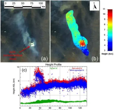
Figure 4.Example of smoke plume height derivation using data from the Multiangle Imaging SpectroRadiometer (MISR) that op-erates on the Terra satellite. This example is extracted from Nel-son et al. (2013). The fire took place on the 12 July 2013 in New Mexico and was observed by MISR at 18:09 UTC. The MISR nadir RGB image showing a smoke plume in grey and a PyroCb in bright white is reported in(a), when the plume stereo-heights derived from the MINX software (Nelson et al., 2013) are shown in(b). MINX height retrieval profiles are shown in(c). Note the dramatic differ-ence in the heights which reach 11–12 km a.s.l. in the PyroCb and stay trapped in a layer around 6–8 km a.s.l. in the vicinity.
but rather has a daytime Equator crossing of around 3 h be-fore Aqua (at 10:30 a.m.).
differ-ently angled MISR views. Post-processed plume heights for more than 25 000 plumes worldwide are accessible through the MISR Plume Height Project1.
Because of its relatively high degree of spatial coverage Kahn et al. (2008) estimate that MISR is at a minimum 40 times more likely to observe a plume that can be linked to a causal fire than CALIOP is. Kahn et al. (2008) explain that MISR and CALIOP are, however, highly complementary since (i) they have different overpass local time as they are on differently orbiting satellites and (ii) CALIOP is able to de-tect optically thin older plumes, while MISR is essentially sensitive to only young plumes exhibiting high contrast with the background. One major drawback of MISR is, however, its relatively early daytime overpass, which limits its ability to observe mature PyroCu as they typically reach their ma-turity in the late afternoon (around 18:00 local time; Fromm et al., 2010). Therefore, MISR-derived plume heights are bi-ased toward lower altitude plumes (Val Martin et al., 2010). The relative lack of highly elevated plume observations from MISR was also reported by Chen et al. (2009). For some of the fire events encountered in their study, Chen et al. (2009) pointed out that the subsequent transport of CO and black carbon were better captured by a crude model of homoge-neously spread emissions up to the top of the troposphere than by an emission profile based on MISR-derived plume heights.
Statistical analyses of MISR-derived plume height data are available in Kahn et al. (2007), Mazzoni et al. (2007), Kahn et al. (2008), Val Martin et al. (2010), Tosca et al. (2011), and Jian and Fu (2014). These studies confirm that the majority of the detected plumes are trapped within the PBL, though geographical location and land cover type have an influence. For example, Kahn et al. (2008) show in their study on fires located in Alaska and the Yukon regions that 5 to 18 % of the fires they observed for the summer 2004 reach the free troposphere, while Tosca et al. (2011) showed that the quasi-totality of fires observed in Borneo and Sumatra (areas im-pacted strongly by peat fires) from 2001 to 2009 (317 fires) were trapped in the PBL. Val Martin et al. (2010) conducted a detailed analysis of the MISR-derived plume height data for fires in North America over a 5-year time period (2002, 2004–2007), finding no clear rules governing the capability of plumes to reach the FT, even when the fires were split per biome. However, Val Martin et al. (2010) show that the percentage of plumes reaching the FT in forest fires (more intense) was larger than crop/grassland fires (less intense).
The along-track scanning radiometer series of sensors have provided a 512 km wide swath stereo-viewing capabil-ity since 1991 (Prata et al., 1990), and recently Fisher et al. (2014) developed an automated stereo-height retrieval algo-rithm (M6) working with data from the advanced along-track scanning radiometer (AATSR). Unlike MINX, M6 is not able
1http://www-misr.jpl.nasa.gov/getData/accessData/
MisrMinxPlumes/
to correct for the plume displacement induced by the am-bient wind. However, it was estimated that such correction would lie in the error of the M6 algorithm (D. Fisher, per-sonal communication, 2015). M6 was applied to AATSR data of Eurasian boreal forests for the April–September period of 4 years between 2008 and 2011 and showed successful com-parisons with collocated observations of smoke layer height derived from CALIOP lidar collections and MINX-derived stereo-heights from MISR. Unfortunately, AATSR also has a bias towards low injection heights since the overpass time is similar to MISR. A wider swath instrument following on from AATSR, the Sea and Land Surface Temperature Ra-diometer (SLSTR), will operate from 2015 (Wooster et al., 2012a). However, this will still not provide daily stereo-data worldwide, and with a limited number of stereo-observations the continuous, direct measurement of smoke plume heights at the global scale appears to be a difficult task.
4.2 Measure of buoyancy flux and fire size
Among the processes inherent to the plume dynamics and listed in Sect. 3, the buoyancy flux and the fire size are the two sets of information needed to characterize the fire. The buoyancy flux generated by the combustion heat release is the primary source of energy responsible of the plume rise. The latent heat, which provides energy to the plume is a sec-ondary source, can only be trigger if the plume reaches its LCL altitude. This LCL altitude can be different from the atmospheric LCL as water content and temperature profiles in plume usually differ from the ambient conditions. To un-derstand the behaviour of the plume dynamics and explain variation in InjH, quantitative information on both the buoy-ant flux and the fire size is therefore needed. The vertical buoyant fluxF is defined as (Viegas, 1998)
F =g(ρ−ρ0)
ρ w=
gR cppo
Qc, (1)
lower than unity, not enough latent heat is able to reach the condensation level.
A bi-spectral algorithm based on middle infrared (MIR) and thermal infrared bands was proposed by Dozier (1981) to estimate the kinetic temperature Tf and the AF areaAf of the black body that would emit the same radiances as the observed fire. According to the Stefan–Boltzmann equation, Qr=σ Tf4, whereσ is the Boltzmann constant. This makes the buoyancy fluxFa direct function ofTf. The Dozier algo-rithm is therefore able to provide all information necessary to characterize the fire (i.e.F =f (Tf)and fire size) as AF area can be used as a proxy for the fire size.
Several implementations of this algorithm have been de-veloped and used with sensor of different resolution: e.g. the BIRD Hot spot Recognition Sensor (185 m, Zhukov et al., 2006), MODIS (1 km, Peterson et al., 2013), or GOES (3 km, Prins et al., 1998). The algorithm is found to be highly sensi-tive to the determination of the long-wave brightness temper-ature background (Giglio and Kendall, 2001) and to a lesser extent to the atmospheric transmittance (Peterson and Wang, 2013). As a result it is not converging for≈10 % of the case. However, this method represents the best available option to estimate buoyancy flux and fire size.
5 Current representation of wildfire emissions injection height in CTMs
A number of studies have determined the very serious im-plications that incorrect InjH estimates have on the ability of CTMs to represent emissions transport (e.g. Hodzic et al., 2007; Turquety et al., 2007). Consequently it may also ef-fect (i) “top-down” emission estimates based on the inversion of observed atmospheric concentrations of biomass burning species (Ichoku and Ellison, 2014) and (ii) radiative forc-ing studies (Ward et al., 2012). This section aims to review the different parameterizations that are currently available to tackle the issue of InjH. They are based either on empirical, deterministic, or statistical models.
5.1 Simple approaches: empirical and/or best-guessed profiles
Because of the complexity of fire plume dynamics, in the early endeavour of biomass burning impact on the atmo-sphere, CTMs often assume a single fixed altitude for all biomass burning emissions usually presuming that all pol-lutants are contained solely within the PBL (e.g. Pfister et al., 2008; Hyer and Chew, 2010). However, such assump-tion cannot represent the observed variability of injecassump-tion height described in Sect. 2. To improve the representation of fire emission at large scale, some studies used a prescribed fixed profile either build on (i) simple hypothetical ratio be-tween boundary layer and tropospheric emission (e.g. Tur-quety et al., 2007; Leung et al., 2007; Elguindi et al., 2010)
or (ii) average local observations (Chen et al., 2009). In the latter work, the authors use the GEOS-Chem model with dif-ferent vertical and temporal emissions distribution to sim-ulate CO and aerosol transport over North America during the fire season 2004. Comparing their simulation results with satellite-, aircraft-, and ground-based measurements, they show that the use of finer temporal distribution enhances long-term transport, while changes due to different InjH im-plementation are small. However, as already mentioned in Sect. 4.1, they also point out that the finer vertical modelled profile emission they implemented is probably affected by MISR observation bias. Most of these early studies do not provide grounded solutions to the problem of fire emission injection role in the atmospheric circulation but rather em-phasize the challenge of developing InjH models.
5.2 Deterministic models 5.2.1 InjH models description
Several studies develop deterministic models capable of be-ing host in CTMs. They are usually based either on phys-ical or dimensional analysis. Goodrick et al. (2013) review the different type of existing plume rise models. In par-ticular, they discuss the use of plume rise models in the framework of the Blue Sky project, which aims to derive smoke emission for air quality models such as the Com-munity Multiscale Air Quality (CMAQ) modelling system. Here, we limit our review to plume rise models originally built to handle fire plume dynamics (see list of physical pro-cesses in Sect. 3). Models like Daysmoke (Achtemeier et al., 2011) or the Briggs equation (Briggs, 1975), which are both available in the CMAQ system, are more suitable for small fires like control burns (Achtemeier et al., 2011) to forecast or prevent emission dispersion and air pollution (i.e. local PM2.5concentration). When used with wildfires, they gener-ally fail to predict large fire impact, certainly because of their weak representation of microphysical processes (Achtemeier et al., 2011) which affect the simulation of PyroCu and Py-roCb plumes. For example, using the Briggs equation and the CMAQ model to simulate fires emission in the USA between 2006 and 2008, Raffuse et al. (2012) show that most of their plumes where below the level expected from remote-sensing measurement.
At present, three parameterizations of plume rise model stand out of the literature, namely Freitas et al. (2007), Rio et al. (2010), and Sofiev et al. (2012). A brief description of each models is reported below.
in the host CTM. In their approach the fire is modelled as an homogeneous circle defined with (i) a size derived from the active fire area of the WF-ABBA GOES prod-uct (Wild Fire Automated Biomass Burning Algorithm; Prins et al., 1998) (ii) and a buoyant flux/CHF calculated as a constant fraction of the total heat. The total heat is set as a prescribed value depending of the vegetation type. The cloud physics is based on a simple microphys-ical module counting three hydrometeors (cloud, rain, ice). Additionally, the horizontal momentum is parame-terized through two entrainment coefficients modelling the effect of (i) the turbulence at the edge of the stack (∝|w|R ; Freitas et al., 2007) and (ii) the drag caused by the ambient wind shear (∝(ue−u)
R ; Freitas et al., 2010). In previous formula,Ris the radius of the plume, andu, ue, andware the horizontal plume, horizontal ambient, and vertical plume velocities respectively.R,u, andw are prognostic variables of the model.
– Rio et al. (2010) implement in the LMDZ model a pa-rameterization based on an eddy diffusivity/mass flux (EDMF) scheme originally developed to model simi-larly shallow convection and dry convection. In com-parison with the implementation of Freitas et al. (2007), this adaptation of EDMF for pyroconvection (pyro-EDMF hereafter) is not based on prognostic equation solved offline but rather evaluates turbulent fluxes pro-duced by the temperature anomaly created by the fire at a sub-grid level and directly adds the source term to the transport equations of the conservative variables of the host CTM. The fire is considered a sub-grid effect and its CHF is modelled as a fraction of the surface sen-sible heat flux averaged over the host model grid cell. The interest of this approach is that the dynamics of the plume is coupled with the ambient atmosphere, so that for example change in the stability of the atmosphere induced by the fire can impact the later development of the plume. In their approach, Rio et al. (2010) apply this extra turbulent flux to the total water, the liquid poten-tial temperature, and the CO2concentration, so that the effect of latent heat can be handle in the CTM, simpli-fying the formulation of the parameterization. The mass flux formulation of pyro-EDMF relies on the definition of two entrainment and detrainment fluxes which are set differently in the PBL and above. Therefore, the mass transfer between the plume and the ambient atmosphere is solved all along the plume. One limitation of the cur-rent version of pyro-EDMF is that ambient shear at sub-grid level is not represented. This certainly overpredicts injection height of small fires which are more sensitive to wind drag.
– Sofiev et al. (2012) use energy balance in the up-draft and some dimensional analysis to develop an equation for the prediction of plume top height based on input
of the FRP, the Brunt–Väisälä frequency, and the PBL height. The equation parameters are fitted using a learn-ing data set of plume height measurement randomly se-lected in the MISR data set. This formulation does not take explicitly into account effects from either entrain-ment, cloud formation, or ambient wind shear. Another limitation of the equation of Sofiev et al. (2012) is in-herent to the selection of the fires used to fit the equa-tion parameters. All events from the learning (and the control) data set used in this study are lower than 4 km. This implies that few PyroCu and certainly no PyroCb are present in the fit of the model.
5.2.2 InjH model validation: fire per fire comparison
Although validation on a fire per fire basis appears to be the best way to ensure the correct functioning of plume rise pa-rameterization, because when implemented in the host model it is highly coupled with the large-scale circulation, few val-idation exist and generally show poor agreement. In their original presentation, PRM and pyro-EDMF have been com-pared with documented fire events as for example the three-dimensional LES simulation of the Chisholm fire (Trentmann et al., 2006), but those tests (Freitas et al., 2010; Rio et al., 2010) are far from being a systematic validation ranging over different fire and atmosphere configuration. Example of those comparisons are reported in Figs. 5 and 6 for PRMv0 and pyro-EDMF respectively.
Sessions et al. (2010) propose the first evaluation of the PRMv0 model. They run a comparison against∼600 fires events captured by MISR that occur in Alaska in spring 2008 during the 10 days of the NASA Arctic Research of the Composition of the Troposphere from Aircraft and Satel-lites (ARCTAS) campaign. They implement two fire initial-ization schemes, both based on WF-ABBA and MODIS data for fire detection but using different temporal representation of the fire size based on either the diurnal cycle estimated in the FLAMBE inventory or kept constant as in the pre-processing of WRF-Chem. They found the best comparison PRMv0-MISR for the FLAMBE-based initialization with a one-to-one correlation of 0.45. They infer the bad response of PRMv0 partly to the quality of their atmospheric profile, emphasize the importance of correct atmospheric profile as already mentioned by Kahn et al. (2007) or Kukkonen et al. (2014).
Figure 5. Results from the one-dimensional plume rise model (PRM) of Freitas et al. (2007, 2010) for a fire burning in(a, c)calm and(b, d)windy atmosphere scenario, as studied by Freitas et al. (2010). The fire has an active fire area (AF area) of 10 ha. The quan-tities shown are vertical velocity (W, ms−1), vertical mass distribu-tion (VMD, %), entrainment acceleradistribu-tion (Ea, 10−1ms−2), buoy-ancy acceleration (Ba, 10−1m s−2), and total condensate water (CW, g kg−1). Model results considering the environmental wind drag are shown in red, whilst those in black depicts the results from simulations disregarding this effect. Grey rectangles indicate the main injection height simulated by the three-dimensional ATHAM model (Trentmann et al., 2006) for the same fire scenario. Fig-ure from Freitas et al. (2010).
or below the PBL. Their comparison is based on a total of 584 plumes selected from the MISR data where the following constraint apply: the plume height is computed immediately above the fire (not from the whole plume as in the original MISR data), the plume is formed of at least five stereo-height retrievals, the clustered MODIS fire pixels are located within 2 km of the plume origin, and the terrain height of the input atmospheric profile do not differ from the terrain elevation used in the MINX software by more than 250 m. Despite this data quality screening, the best one-to-one correlation they obtain is about 0.3.
In their approach, Sofiev et al. (2012) use the whole MISR data set (counting 2000 fires at that time) without any filter-ing. Because of its derivation based on an optimization pro-cedure, their model compares relatively well to the selected MISR data. However, when compared with the current full data set for North America, results are not as good, show-ing a constant underestimation of plume height, in particular for high plumes. Figure 7 shows together a comparison of our implementation of the Sofiev model against (i) the origi-nal version of the model (ii) and against 3206 “good” quality
flag fires of the North American subset of the MISR data set. Even if our implementation of the model exhibits a slight positive bias (certainly due to a different estimation of the PBL height which we read from the diagnostic products of the forecast run of ECMWF, 2012), our comparison with the MISR data shows a strong negative bias of the model. Sim-ilar behaviour was also shown for PRMv1 in the study of Val Martin et al. (2012). When compared with the PRMv1 sensitivity study of Val Martin et al. (2012) (Fig. 7b and Fig. 2 of Val Martin et al., 2012, show the same metrics), the Sofiev model does not perform better, showing a regres-sion line slope of 0.4 for the Sofiev model against 0.8 for the best set-up of PRMv1. Note however that here we are using a larger extent of the MISR data set than in Val Martin et al. (2012).
5.2.3 InjH models implementation
Despite the lack of conclusive fire per fire validation (see previous section), plume rise parameterizations have been implemented in several regional and large-scale models. PRMv0 has been coupled with the Weather Research and Forecasting (WRF) Model (Sessions et al., 2010; Grell et al., 2011; Pfister et al., 2011) and the Coupled Aerosol and Tracer Transport model to the Brazilian developments on the Regional Atmospheric Modelling System (CATT-BRAMS; Freitas et al., 2009; Longo et al., 2010). Additionally, pyro-EDMF is present in the mesoscale non-hydrostatic model (MesoNH; Strada et al., 2012) and the general circulation model LMDZ (Rio et al., 2010). See Table 1 of Val Martin et al. (2012) for a more complete list of atmospheric models with plume rise parameterization.
Several studies highlight the need to inject fire emission at high altitude (Turquety et al., 2007; Elguindi et al., 2010), and recent in situ (Cammas et al., 2009) and remote-sensing (Fromm et al., 2010) observations show the frequent occur-rence of large PyroCb. However, the role of plume rise pa-rameterization in transport of fire emission at a large scale in CTM simulation is still a matter of debate. A list of different conclusion from recent studies is reported below.
– Sessions et al. (2010) who are using PRMv0 embed-ded in WRF-Chem, simulate 10 days of the Spring 2008 ARCTAS campaign. As for their fire per fire comparison (see previous section), they show that among their two initialization schemes, the use of the FLAMBE-based initialization gives the best emission transport when compared with the Atmospheric In-fraRed Sounder (AIRS) total columns CO and CALIOP aerosol profiles. Also a comparison with coarser injec-tion schemes (distributing all fire emissions in the PBL or between altitude levels of 3 and 5 km) shows that the use of PRMv0 is improving the simulation.
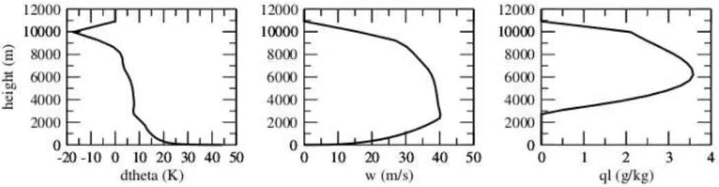
lo-Figure 6.Smoke plume characteristics for the Chisholm fire, as simulated by pyro-EDMF: virtual potential temperature (K), vertical velocity excess (m s−1), and cloud liquid water (g kg−1) are shown. Figure from Rio et al. (2010).
Figure 7.Comparison of our implementation of the plume rise parameterization of Sofiev et al. (2012) to(a)the original results from Sofiev et al. (2012) for the same fires and(b)plume stereo-height retrievals extracted from the North American subset of the (MISR) plume height project data Nelson et al. (2013), derived using the MINX tool as shown in Fig. 4. Our implementation of the Sofiev et al. (2012) model differs from the original in its definition of the PBL height, which in our approach is extracted from the diagnostic product of ECMWF forecast runs (ECMWF, 2012). See Figs. 9 and 10 for a statistical overview of the North American MISR data set. Note that the Sofiev et al. (2012) model did not retrieve simulated plume heights for all the 3320 selected fires of that data set. For 114 fires, either the Brunt–Väisälä frequency could not be retrieved or the FRP of the most powerful pixel listed in the MISR product was unavailable (see Sofiev et al., 2012, for details in the initialization of the model). Panel(b)shows the same metrics as Fig. 2 of Val Martin et al. (2012), i.e. two-sided regression line (grey), box plots of the distributions of model heights and 500 m resolution MISR heights for central 67 % (box) and central 90 % (cap), median distribution regression line (magenta), and 1:1 relationship (dashed black).
cated in the tropics between 5 and 20◦south. Fires loca-tions and emissions are estimated from the burnt area product L3JRC while fire activity is idealized with a constant fire area of 2 km2 and a Gaussian diurnal cy-cle peaking at 15:45 LTC. Figure 8 show results from their simulations for different values of their parameter β which defines the ratio between the entrainment (ǫ) and detrainment (δ) coefficients for the levels located above the PBL. Bothǫ andδ are set constant (no alti-tude dependence) and inversely proportional to the base of the plume radius. Their results show that pyro-EDMF is sensitive to the value of the parameter β as the de-trainment altitude control the final spread of the smoke emission. Rio et al. (2010) also show that LMDZ was able to predict the daily tropospheric emission (DTE) of CO2(daily variation of CO2in the troposphere) ob-served by Chédin et al. (2005). However, their simulated
amplitude of DTE for southern Africa is much lower than the observed value. Rio et al. (2010) focus only on tropical fire in Africa. In the tropics, natural con-vection is more active than in higher latitude and fire-generated heat and vertical water transport could be a trigger to initiate natural convection (private communi-cation Ben Johnson). Testing pyro-EDMF on a boreal forest fire scenario would be interesting.
– Grell et al. (2011) run the WRF model coupled with PRMv0 initialized with fire size input data estimated from in situ measurement. Running WRF at cloud-resolving scale over Alaska for 2 days for summer 2004, they show that the use of PRMv0 improves the results when compared to radio sounding.
Figure 8.Simulations performed using the pyro-EDMF plume rise model of Rio et al. (2010) for sub-Saharan Africa between 10 and 30 July 2006. In the upper panel,(a)shows the maximal injection height of CO2emissions simulated with the LMDZ model and pyro-EDMF between 5 and 20◦S over the 20 days of the simulation.(b)reports the maximal injection height (green), mean injection height of emissions injected above the boundary layer height (red), and mean boundary layer height (black) averaged between 5 and 20◦S altitude and over the 20 days of the simulation.(c)shows the percentage of cases for which the injection height passes the boundary layer height. In the lower panel,(e)shows the averaged vertical distribution of CO2mixing ratio (ppmv) for the same reference simulation and(d)for simulations without pyro-EDMF and(f)with pyro-EDMF set up with a lower value of the ratioβ=entrainment
detrainment=0.1 (right). The reference simulation in(e)uses a value ofβ=0.4. Figure from Rio et al. (2010).
month of the summer of 2008, coinciding with the ARCTAS campaign. WRF-Chem was also coupled with the global Model for OZone and Related Chemical Tracers (MOZART) which is used to provide boundary conditions. Such a system allows the estimation of the relative importance of local sources versus pollution in-flow on the distribution of CO at the surface and in the free troposphere. Fire emissions are based on the FINN inventory (Wiedinmyer et al., 2011) which in their case study shows a clear underestimation of CO emission over California. Model results are compared against air-borne and ground measurement of CO as well as CO total column from MOPITT. In the perspective of InjH modelling, Pfister et al. (2011) show that (i) in their case study PRMv0 injects half of the fire in the FT and cap-tures the timing and location of fire plume well when compared to airborne CO measurements (ii) and that their comparison with surface measurement is impacted by a large underestimation of CO fire emission in the FINN inventory.
The conclusions of these studies emphasize the fact that the evaluation of plume rise effects on large-scale atmo-spheric transport simulation is a challenging task. As emis-sion transport is dependent of both quantity and the geo-graphical location of the injection, both emission inventory and local condition (i.e. atmospheric profile) need to be cor-rectly input to allow the evaluation of InjH estimation.
5.3 Statistical models
As an alternative to the unreliable prediction of the PRM model, a statistically based approach using 584 plume height measurements of the MISR data set was presented by Val Martin et al. (2012). Classifying observed fires between low (<1 km), medium (<2.5 km), and high (>2.5 km) plumes, they derive per biome the mean and standard devi-ation of FRP (MW) and atmospheric stable layer strength (K km−1) for each plume height class (See Table 4 of Val Martin et al., 2012). Although this approach is attractive because of its inexpensive computational cost, its implemen-tation appears to be difficult as most of the standard devia-tion for FRP and the stable layer strength are extremely high, yielding crossover between the characterization of FRP and stable layer strength ranges of the different plume categories and therefore large uncertainty on the InjH estimation.
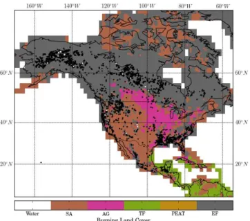
Figure 9. Fire locations contained within the Multi-angle Imag-ing SpectroRadiometer (MISR) plume height data set of Nelson et al. (2013) over North America for the time period 2001–2008 (black dots). White dots indicate the locations of the 22 fires plumes classed as having a plume height in excess of 4.5 km. The map in the background shows the land cover used within the GFEDv3 biomass burning emissions inventory of van der Werf et al. (2010) where SA, AG, TF, PEAT, and EF stand for savannah, agriculture, tropical forest, peat land, and extra tropical forest respectively.
of injection in the troposphere, no real model is formulated and their conclusion highlights the potential importance of atmospheric stability in the plume rise (which they do not take into account).
To our knowledge, no statistically based models has al-ready been implemented in CTMs. However, as their CPU cost would remain relatively low compared to any determin-istic models, they show a great potential for implementation in large-scale model, in particular in climate model. How-ever, their derivation is entirely relying on the good quality of their learning data set.
6 Summary and conclusions
Weakly burning landscape-scale fires appear to release their smoke mainly into the planetary boundary layer, but larger and/or more intensely burning wildfires produce smoke columns that can rise rapidly and semi-vertically above the source region, driven by the intense heat and convective en-ergy released by the burning vegetation. These columns of hot smoke entrains cooler ambient air, developing into a ris-ing plume within which the trace gases and aerosols are transported to potentially quite high altitudes, in the most extreme cases into the stratosphere. The characteristics of these rising plumes, and in particular the height that they reach before releasing the majority of the smoke burden,
Figure 10.Distribution of FRP(a), active fire area(b), top plume height(c), and local time observation(d)for the 3320 fires of the current North American subset of the Multi-angle Imaging Spectro-Radiometer (MISR) plume height project data set of Nelson et al. (2013) derived using the MINX tool shown in Fig. 4.
are now acknowledged as an important control on the atmo-spheric transport of emissions from certain of these larger fire events (Colarco et al., 2004; Turquety et al., 2007; Rio et al., 2010). However, results comparing model-based esti-mates of smoke plume rise parameter to actual plume height observations made from satellite EO instruments (e.g. Ichoku et al., 2012) do not yet provide a strong quantitative agree-ment (Val Martin et al., 2012). Furthermore, the degree of improvement given by actually including plume rise param-eterizations in atmospheric chemistry transport models can be difficult to interpret due to the complex interactions with other atmospheric processes Chen et al. (2009).
dy-Figure 11.Overview of the highest fire plumes present in the current North American subset of the MISR plume height data set of Nelson et al. (2013), derived using the MINX tool shown in Fig. 4. The reference of this fire in the MISR data set is O45791-B41-P1, and it was observed in the Northwest Territories (Canada) on 27 July 2008. It shows the nadir image recorded by MISR, together with the plume contour set by the operator of the MINX software(a), the estimated wind direction (yellow arrow ina), and the stereo-height retrieval(b). Part of the image is black as the fire was located on the edge of the MISR swath. Images are taken from the MISR plume height project website (see footnote 1).
Figure 12.Images from the wider-swath Moderate Resolution Imaging Spectroradiometer (MODIS) for the same fire as in Fig. 11 at the same time. MODIS is mounted on the same Terra satellite as MISR (see Sect. 4.1).(a)is the false colour composite image of the area observed.(b)is the Middle Infra-Red brightness temperature.(c)is the optical cloud phase properties of the version 6 of the MODIS cloud product Platnick et al. (2003). Cross markers in(a)and(c)(red and green respectively) denote the location of MODIS pixels detected as containing active fire in the MODIS MOD14 active fire product of Giglio et al. (2003).
namics, using inputs regarding the fire characteristics that are available from EO satellites in near real time and with con-current measurements of fire activity and plume height from single fire events available to validate the resulting system (and reduce any impact from larger-scale transport effects that influence comparisons of downwind plume characteris-tics).
Despite a demonstrated diurnal bias of MISR-derived plume heights towards lower plumes (Val Martin et al., 2010), the current MISR data set for North America counts 22 fires with plume top higher that 4.5 km (see Figs. 9 and 10 for an overview of the current MISR data over North Amer-ica).
carefully selected evaluation data set, the validation of this PRM model fails to show very convincing results. Neverthe-less, in future, such validation (or optimization) of plume rise models should continue to pay attention to the quality of the evaluation data sets, including the following questions.
i. Are the fire activity (FRP) and the plume dynamics (plume top height) linked? A time delay is necessary for the plume to dynamically adjust to change in the forcing induced by the energy release by the fire. For example, during the simulation of PyroCb of the Chisholm fire by the ATHAM model, it takes 40 min for the plume to reach its stationary altitude with a constant forcing (Trentmann et al., 2006). As the smoke plumes observed by MISR are more likely in a relatively early stage of development due to the morning overpass of the Terra satellite (see Sect. 4.1.2), the effect of this time lag might be even more important than if fires were ran-domly observed at any time of their development. ii. Is the radiation of the fire affecting by absorption from
the plume? In low ambient wind conditions, the fire plume is often located just above the fire and in case of large fires this might mask some of the fire-emitted radiation due to the thick aerosol layer causing signifi-cant scattering and/or absorption of the radiant energy, possibly causing underestimation of FRP and unreliable CHF and fire size retrievals using the Dozier algorithm. As an example, we note that the fire from the Northern American MISR plume height data set observed with the highest plume height of 12 km (see Fig. 10c) is re-ported to have a relatively low total FRP of 6 GW, when compare with the FRP distribution of the whole MISR data set (see Fig. 10a). The FRP is here determined as in Paugam et al. (2015): it is the FRP of the strongest cluster in the vicinity of the plume, in this case the top cluster in Fig. 12a. Figure 12b shows the optical cloud phase properties of the MODIS cloud product (Platnick et al., 2003) for this same fire. A large part of the plume is formed of ice, which lets us assume that we are in the presence of a PyroCb event. This means that the plume is formed of liquid water and ice particles that could be absorbing part of the MIR signal emitted by the fire. A close inspection of the MODIS MIR band (Fig. 12c) shows that in this particular event all high radiance pix-els are outside the plume and that the fire detection al-gorithm of the MOD14 product misses a part of the fire front. This underestimation is even further accentuated in the official MISR data set as the plume contour set by the MINX operator includes only a part of the detected fire pixels (see Fig. 11). An even more extreme scenario is shown in Fig. 14 of Kahn et al. (2007), where no fire pixels were found for a high plume (marked P2 in their figure) which occurred in Québec on 6 July 2002. In these particularly extreme fire cases, it seems that fire pixels attached to the plume could be located
under-neath it and remain undetected by the MODIS active fire product.
Despite these difficulties, the range of relevant data pro-vided on actively burning fires and their smoke plumes by EO satellites continues to grow (e.g. Ichoku et al., 2012). For example, GOES-R (Schmit et al., 2005) and Himawari-8 (Kurino, 2012) will provide capabilities similar to MODIS, with a temporal frequency potentially as high as 30 s, while Suomi NPP carrying VIIRS (Schroeder et al., 2014) and TET-1/BIRDS (Lorenz et al., 2012) will provide thermal bands with resolution up to 375 m. This will allow for de-tailed observations of pyroconvection during peak burning hours. These improving capabilities, together with continu-ing advances in the extent to which plume rise models can be parameterized and incorporated into large-scale atmospheric CTMs (Peterson et al., 2014; Paugam et al., 2015), can be ex-pected to continue to advance the accuracy of smoke plume injection estimates and the resulting impact on long-range atmospheric transport of these globally important emissions.
Acknowledgements. This study was supported by the NERC
grant NE/E016863/1, by the NERC National Centre for Earth Observation (NCEO), and by the EU in the FP7 and H2020 projects MACC-II and MACC-III (contracts 283576 and 633080). The authors want also to thank M. Sofiev for sharing results from the implementation of his plume rise parameterization.
Edited by: R. Engelen
References
Achtemeier, G. L., Goodrick, S. A., Liu, Y., Garcia-Menendez, F., Hu, Y., and Odman, M. T.: Modeling Smoke Plume-Rise and Dispersion from Southern United States Pre-scribed Burns with Daysmoke, Atmosphere, 2, 358–388, doi:10.3390/atmos2030358, 2011.
Amiridis, V., Giannakaki, E., Balis, D. S., Gerasopoulos, E., Pytharoulis, I., Zanis, P., Kazadzis, S., Melas, D., and Zerefos, C.: Smoke injection heights from agricultural burning in Eastern Europe as seen by CALIPSO, Atmos. Chem. Phys., 10, 11567– 11576, doi:10.5194/acp-10-11567-2010, 2010.
Andreae, M. O. and Merlet, P.: Emission of trace gases and aerosols from biomass burning, Global Biogeochem. Cy., 15, 955–966, doi:10.1029/2000GB001382, 2001.
Andreae, M. O., Rosenfeld, D., Artaxo, P., Costa, A. A., Frank, G. P., Longo, K. M., and Silva-Dias, M. A. F.: Smoking Rain Clouds over the Amazon, Science, 303, 1337–1342, doi:10.1126/science.1092779, 2004.
Briggs, G. A.: Plume Rise Equations, in: Lectures on air pollu-tion and environmental impact analyses, edited by: Haugen, D., AMS: Boston, MA, USA, 59–111, 1975.
Cammas, J.-P., Brioude, J., Chaboureau, J.-P., Duron, J., Mari, C., Mascart, P., Nédélec, P., Smit, H., Pätz, H.-W., Volz-Thomas, A., Stohl, A., and Fromm, M.: Injection in the lower strato-sphere of biomass fire emissions followed by long-range trans-port: a MOZAIC case study, Atmos. Chem. Phys., 9, 5829–5846, doi:10.5194/acp-9-5829-2009, 2009.
Chatfield, R. B. and Delany, A. C.: Convection links biomass burn-ing to increased tropical ozone: However, models will tend to overpredict O3, J. Geophysical Res.-Atmos., 95, 18473–18488, doi:10.1029/JD095iD11p18473, 1990.
Chédin, A., Serrar, S., Scott, N. A., Pierangelo, C., and Ciais, P.: Impact of tropical biomass burning emissions on the diurnal cycle of upper tropospheric CO2 retrieved from NOAA 10 satellite observations, J. Geophys. Res.-Atmos., 110, doi:10.1029/2004JD005540, 2005.
Chen, Y., Li, Q., Randerson, J. T., Lyons, E. A., Kahn, R. A., Nel-son, D. L., and Diner, D. J.: The sensitivity of CO and aerosol transport to the temporal and vertical distribution of North Amer-ican boreal fire emissions, Atmos. Chem. Phys., 9, 6559–6580, doi:10.5194/acp-9-6559-2009, 2009.
Coheur, P.-F., Clarisse, L., Turquety, S., Hurtmans, D., and Cler-baux, C.: IASI measurements of reactive trace species in biomass burning plumes, Atmos. Chem. Phys., 9, 5655–5667, doi:10.5194/acp-9-5655-2009, 2009.
Colarco, P. R., Schoeberl, M. R., Doddridge, B. G., Marufu, L. T., Torres, O., and Welton, E. J.: Transport of smoke from Cana-dian forest fires to the surface near Washington, D.C.: Injection height, entrainment, and optical properties, J. Geophys. Res.-Atmos., 109, doi:10.1029/2003JD004248, 2004.
Damoah, R., Spichtinger, N., Servranckx, R., Fromm, M., Elo-ranta, E. W., Razenkov, I. A., James, P., Shulski, M., Forster, C., and Stohl, A.: A case study of pyro-convection using transport model and remote sensing data, Atmos. Chem. Phys., 6, 173– 185, doi:10.5194/acp-6-173-2006, 2006.
Dirksen, R. J., Folkert Boersma, K., de Laat, J., Stammes, P., van der Werf, G. R., Val Martin, M., and Kelder, H. M.: An aerosol boomerang: Rapid around-the-world transport of smoke from the December 2006 Australian forest fires ob-served from space, J. Geophys. Res.-Atmos., 114, D21201, doi:10.1029/2009JD012360, 2009.
Dozier, J.: A method for satellite identification of surface temper-ature fields of subpixel resolution, Remote Sens. Environ., 11, 221–229, doi:10.1016/0034-4257(81)90021-3, 1981.
ECMWF: IFS documentation Part IV: Physical Pro- cesses, Tech. Rep. CY38r1, European Center for Medium-Range Weather Forecasts, Shinfield Park, Reading, UK, available at: http: //old.ecmwf.int/research/ifsdocs/CY38r1/IFSPart4.pdf (last ac-cess: March 2015), 2012.
Elguindi, N., Clark, H., Ordóñez, C., Thouret, V., Flemming, J., Stein, O., Huijnen, V., Moinat, P., Inness, A., Peuch, V.-H., Stohl, A., Turquety, S., Athier, G., Cammas, J.-P., and Schultz, M.: Cur-rent status of the ability of the GEMS/MACC models to repro-duce the tropospheric CO vertical distribution as measured by MOZAIC, Geosci. Model Dev., 3, 501–518, doi:10.5194/gmd-3-501-2010, 2010.
Fisher, D., Muller, J.-P., and Yershov, V.: Automated Stereo Re-trieval of Smoke Plume Injection Heights and ReRe-trieval of Smoke Plume Masks From AATSR and Their Assessment With CALIPSO and MISR, Geoscience and Remote Sens., 52, 1249– 1258, doi:10.1109/TGRS.2013.2249073, 2014.
Freeborn, P. H., Wooster, M. J., Hao, W. M., Ryan, C. A., Nord-gren, B. L., Baker, S. P., and Ichoku, C.: Relationships between energy release, fuel mass loss, and trace gas and aerosol emis-sions during laboratory biomass fires, J. Geophys. Res.-Atmos/, 113, D01301, doi:10.1029/2007JD008679, 2008.
Freitas, S. R., Longo, K. M., and Andreae, M. O.: Impact of in-cluding the plume rise of vegetation fires in numerical simula-tions of associated atmospheric pollutants, Geophys. Res. Lett., 33, doi:10.1029/2006gl026608, 2006.
Freitas, S. R., Longo, K. M., Chatfield, R., Latham, D., Silva Dias, M. A. F., Andreae, M. O., Prins, E., Santos, J. C., Gielow, R., and Carvalho Jr., J. A.: Including the sub-grid scale plume rise of veg-etation fires in low resolution atmospheric transport models, At-mos. Chem. Phys., 7, 3385–3398, doi:10.5194/acp-7-3385-2007, 2007.
Freitas, S. R., Longo, K. M., Silva Dias, M. A. F., Chatfield, R., Silva Dias, P., Artaxo, P., Andreae, M. O., Grell, G., Rodrigues, L. F., Fazenda, A., and Panetta, J.: The Coupled Aerosol and Tracer Transport model to the Brazilian developments on the Re-gional Atmospheric Modeling System (CATT-BRAMS) – Part 1: Model description and evaluation, Atmos. Chem. Phys., 9, 2843– 2861, doi:10.5194/acp-9-2843-2009, 2009.
Freitas, S. R., Longo, K. M., Trentmann, J., and Latham, D.: Tech-nical Note: Sensitivity of 1-D smoke plume rise models to the inclusion of environmental wind drag, Atmos. Chem. Phys., 10, 585–594, doi:10.5194/acp-10-585-2010, 2010.
Fromm, M., Bevilacqua, R., Servranckx, R., Rosen, J., Thayer, J. P., Herman, J., and Larko, D.: Pyro-cumulonimbus injection of smoke to the stratosphere: Observations and impact of a super blowup in northwestern Canada on 3–4 August 1998, J. Geophys. Res.-Atmos., 110, D08205, doi:10.1029/2004JD005350, 2005. Fromm, M., Lindsey, D. T., Servranckx, R., Yue, G., Trickl, T.,
Sica, R., Doucet, P., and Godin-Beekmann, S.: The Untold Story of Pyrocumulonimbus, B. Am. Meteorol. Soc., 91, 1193–1209, doi:10.1175/2010BAMS3004.1, 2010.
Fromm, M. D. and Servranckx, R.: Transport of forest fire smoke above the tropopause by supercell convection, Geophys. Res. Lett., 30, doi:10.1029/2002GL016820, 2003.
Giglio, L. and Kendall, J. D.: Application of the Dozier re-trieval to wildfire characterization: a sensitivity analysis, Remote Sens. Environ., 77, 34–49, doi:10.1016/S0034-4257(01)00192-4, 2001.
Giglio, L. and Schroeder, W.: A global feasibility assessment of the bi-spectral fire temperature and area retrieval us-ing {MODIS} data, Remote Sens. Environ., 152, 166–173, doi:10.1016/j.rse.2014.06.010, 2014.
Giglio, L., Descloitres, J., Justice, C. O., and Kaufman, Y. J.: An Enhanced Contextual Fire Detection Algorithm for {MODIS}, Remote Sens. Environ., 87, 273–282, doi:10.1016/S0034-4257(03)00184-6, 2003.
Gonzi, S. and Palmer, P. I.: Vertical transport of surface fire emissions observed from space, J. Geophys. Res.-Atmos., 115, D02306, doi:10.1029/2009JD012053, 2010.
Gonzi, S., Palmer, P. I., Paugam, R., Wooster, M., and Deeter, M. N.: Quantifying pyroconvective injection heights using ob-servations of fire energy: sensitivity of spaceborne observa-tions of carbon monoxide, Atmos. Chem. Phys., 15, 4339–4355, doi:10.5194/acp-15-4339-2015, 2015.
Goodrick, S. L., Achtemeier, G. L., Larkin, N. K., Liu, Y., and Strand, T. M.: Modelling smoke transport from wildland fires: a review, Int. J. Wildland Fire, 22, 83–94, 10.1071/WF11116, 2013.
Grell, G., Freitas, S. R., Stuefer, M., and Fast, J.: Inclusion of biomass burning in WRF-Chem: impact of wildfires on weather forecasts, Atmos. Chem. Phys., 11, 5289–5303, doi:10.5194/acp-11-5289-2011, 2011.
Guan, H., Esswein, R., Lopez, J., Bergstrom, R., Warnock, A., Follette-Cook, M., Fromm, M., and Iraci, L. T.: A multi-decadal history of biomass burning plume heights identified using aerosol index measurements, Atmos. Chem. Phys., 10, 6461–6469, doi:10.5194/acp-10-6461-2010, 2010.
Hodzic, A., Madronich, S., Bohn, B., Massie, S., Menut, L., and Wiedinmyer, C.: Wildfire particulate matter in Europe during summer 2003: meso-scale modeling of smoke emissions, trans-port and radiative effects, Atmos. Chem. Phys., 7, 4043–4064, doi:10.5194/acp-7-4043-2007, 2007.
Hyer, E. J. and Chew, B. N.: Aerosol transport model evaluation of an extreme smoke episode in Southeast Asia, Atmos. Environ., 44, 1422–1427, doi:10.1016/j.atmosenv.2010.01.043, 2010. Ichoku, C. and Ellison, L.: Global top-down smoke-aerosol
emis-sions estimation using satellite fire radiative power measure-ments, Atmos. Chem. Phys., 14, 6643–6667, doi:10.5194/acp-14-6643-2014, 2014.
Ichoku, C., Kahn, R., and Chin, M.: Satellite contribu-tions to the quantitative characterization of biomass burning for climate modeling, Atmos. Res., 111, 1–28, doi:10.1016/j.atmosres.2012.03.007, 2012.
Jian, Y. and Fu, T.-M.: Injection heights of springtime biomass-burning plumes over peninsular Southeast Asia and their im-pacts on long-range pollutant transport, Atmos. Chem. Phys., 14, 3977–3989, doi:10.5194/acp-14-3977-2014, 2014.
Johnson, B. T., Osborne, S. R., Haywood, J. M., and Harrison, M. A. J.: Aircraft measurements of biomass burning aerosol over West Africa during DABEX, J. Geophys. Res.-Atmos., 113, D00C06, doi:10.1029/2007JD009451, 2008.
Justice, C., Giglio, L., Korontzi, S., Owens, J., Morisette, J., Roy, D., Descloitres, J., Alleaume, S., Petitcolin, F., and Kauf-man, Y.: The {MODIS} fire products the Moderate Resolu-tion Imaging Spectroradiometer (MODIS): a new generaResolu-tion of Land Surface Monitoring, Remote Sens. Environ., 83, 244–262, doi:10.1016/S0034-4257(02)00076-7, 2002.
Kahn, R. A., Li, W.-H., Moroney, C., Diner, D. J., Martonchik, J. V., and Fishbein, E.: Aerosol source plume physical characteristics from space-based multiangle imaging, J. Geophys. Res.-Atmos., 112, D11205, doi:10.1029/2006JD007647, 2007.
Kahn, R. A., Chen, Y., Nelson, D. L., Leung, F.-Y., Li, Q., Diner, D. J., and Logan, J. A.: Wildfire smoke injection heights: Two perspectives from space, Geophys. Res. Lett., 35, doi:10.1029/2007GL032165, 2008.
Kaiser, J. W., Heil, A., Andreae, M. O., Benedetti, A., Chubarova, N., Jones, L., Morcrette, J.-J., Razinger, M., Schultz, M. G., Suttie, M., and van der Werf, G. R.: Biomass burning emis-sions estimated with a global fire assimilation system based on observed fire radiative power, Biogeosciences, 9, 527–554, doi:10.5194/bg-9-527-2012, 2012.
Kaskaoutis, D., Kharol, S. K., Sifakis, N., Nastos, P., Sharma, A. R., Badarinath, K., and Kambezidis, H.: Satellite monitoring of the biomass-burning aerosols during the wildfires of August 2007 in Greece: Climate implications, Atmos. Environ., 45, 716–726, doi:10.1016/j.atmosenv.2010.09.043, 2011.
Keeley, J. E.: Fire intensity, fire severity and burn severity: a brief review and suggested usage, Int. J. Wildland Fire, 18, 116–126, doi:10.1071/wf07049, 2009.
Kukkonen, J., Nikmo, J., Sofiev, M., Riikonen, K., Petäjä, T., Virkkula, A., Levula, J., Schobesberger, S., and Webber, D. M.: Applicability of an integrated plume rise model for the disper-sion from wild-land fires, Geosci. Model Dev., 7, 2663–2681, doi:10.5194/gmd-7-2663-2014, 2014.
Kurino, T.: Future Plan and Recent Activities for the Japanese Follow-on Geostationary Meteorological Satellite Himawari-8/9, AGU Fall Meeting Abstracts, p. 3, 2012.
Labonne, M., Bréon, F.-M., and Chevallier, F.: Injection height of biomass burning aerosols as seen from a spaceborne lidar, Geo-phys. Res. Lett., 34, doi:10.1029/2007GL029311, 2007. Latham, D.: PLUMP: A one-dimensional plume predictor and cloud
model for fire and smoke managers, Tech. Rep. INT–GTR–314, Intermountain Research Station, USDA Forest Service, 1994. Leung, F.-Y. T., Logan, J. A., Park, R., Hyer, E., Kasischke, E.,
Streets, D., and Yurganov, L.: Impacts of enhanced biomass burning in the boreal forests in 1998 on tropospheric chem-istry and the sensitivity of model results to the injection height of emissions, J. Geophys. Res.-Atmos., 112, D10313, doi:10.1029/2006JD008132, 2007.
Longo, K. M., Freitas, S. R., Andreae, M. O., Setzer, A., Prins, E., and Artaxo, P.: The Coupled Aerosol and Tracer Transport model to the Brazilian developments on the Regional Atmo-spheric Modeling System (CATT-BRAMS) – Part 2: Model sen-sitivity to the biomass burning inventories, Atmos. Chem. Phys., 10, 5785–5795, doi:10.5194/acp-10-5785-2010, 2010.
Lorenz, E., Hoffmann, A., Oertel, D., Tiemann, J., and Halle, W.: Upcoming and prospective fire monitoring mis-sions based on the heritage of the BIRD (bi-spectral in-frared detection) satellite, in: Geoscience and Remote Sens-ing Symposium (IGARSS), 2012 IEEE International, 225–228, doi:10.1109/IGARSS.2012.6351597, 2012.
Luderer, G., Trentmann, J., Winterrath, T., Textor, C., Herzog, M., Graf, H. F., and Andreae, M. O.: Modeling of biomass smoke injection into the lower stratosphere by a large forest fire (Part II): sensitivity studies, Atmos. Chem. Phys., 6, 5261–5277, doi:10.5194/acp-6-5261-2006, 2006.
Mazzoni, D., Logan, J. A., Diner, D., Kahn, R., Tong, L., and Li, Q.: A data-mining approach to associating {MISR} smoke plume heights with {MODIS} fire measurements, Remote Sens. Envi-ron., 107, 138–148, doi:10.1016/j.rse.2006.08.014, 2007. McCarter, R. J. and Broido, A.: Radiative and convective energy
from wood crib fires, Pyrodynamics, 2, 65–85, 1965.