NO<sub>3</sub> radical measurements in a polluted marine environment: links to ozone formation

(1)

ACPD

9, 24531–24585, 2009

NO₃ radical measurements in a

polluted marine environment

R. McLaren et al.

Title Page

Abstract Introduction

Conclusions References

Tables Figures

◭ ◮

Back Close

Full Screen / Esc

Printer-friendly Version

Interactive Discussion

Atmos. Chem. Phys. Discuss., 9, 24531–24585, 2009 www.atmos-chem-phys-discuss.net/9/24531/2009/ © Author(s) 2009. This work is distributed under the Creative Commons Attribution 3.0 License.

Atmospheric Chemistry and Physics Discussions

This discussion paper is/has been under review for the journal Atmospheric Chemistry and Physics (ACP). Please refer to the corresponding final paper in ACP if available.

NO

₃

radical measurements in a polluted

marine environment: links to ozone

formation

R. McLaren1, P. Wojtal1, D. Majonis1, J. McCourt1, J. D. Halla1, and J. Brook2

1

Centre for Atmospheric Chemistry, York University, North York, ON, Canada 2

Air Quality Research Division, Environment Canada, Toronto, ON, Canada

Received: 20 October 2009 – Accepted: 4 November 2009 – Published: 18 November 2009

Correspondence to: R. McLaren (rmclaren@yorku.ca)

(2)

ACPD

9, 24531–24585, 2009

R. McLaren et al.

Title Page

Tables Figures

◭ ◮

Back Close

Full Screen / Esc

Abstract

Nighttime chemistry in polluted regions is dominated by the nitrate radical (NO3) in-cluding its direct reaction with natural and anthropogenic hydrocarbons, its reaction with NO₂ to form N₂O₅, and subsequent reactions of N₂O₅ to form HNO₃ and chlo-rine containing photolabile species. We report nighttime measurements of NO3, NO2,

5

and O3, in the polluted marine boundary layer southwest of Vancouver, BC during a three week study in summer of 2005. The concentration of N₂O₅was calculated using the well known equilibrium, NO3+NO2↔N2O5. Median overnight mixing ratios of NO3, N2O5and NO2were 10.3 ppt, 122 ppt and 8.3 ppb with median N2O5/NO3molar ratios of 13.1 and median nocturnal partitioning of 4.9%. Due to the high levels of NO₂ that

10

can inhibit approach to steady-state, we use a method for calculating NO₃ lifetimes that does not assume the steady-state approximation. Median and average lifetimes of NO3in the NO3-N2O5nighttime reservoir were 1.1–2.3 min. We have determined noc-turnal profiles of the pseudo first order loss coe_fficient of NO₃ and the first order loss coefficients of N2O5 by regression of the NO3 inverse lifetimes with the [N2O5]/[NO3]

15

ratio. Direct losses of NO3 are highest early in the night, tapering off as the night proceeds. The magnitude of the first order loss coe_fficient of N₂O₅ is consistent with recommended homogeneous rate coefficients for reaction of N2O5 with water vapor early in the night, but increases significantly in the latter part of the night when relative humidity increases beyond 75%, consistent with heterogeneous reactions of N₂O₅with

20

sea salt and/or other aerosols with rate constant khet=1.2×10− 3

s−1. Analysis indicates that a correlation exists between overnight integrated N2O5concentrations in the ma-rine boundary layer, a surrogate for the accumulation of chloma-rine containing photolabile species, and maximum 1-h average O3at stations in the Lower Fraser Valley the next day when there is clear evidence of a sea breeze transporting marine air into the

val-25

ley. The range of maximum 1-h average O₃ increase attributable to the correlation is

∆O3=+1.1 to +8.3 ppb throughout the study for the average of 20 stations, although higher increases are seen for stations far downwind of the coastal urban area. The

(3)

ACPD

9, 24531–24585, 2009

R. McLaren et al.

Title Page

Tables Figures

◭ ◮

Back Close

Full Screen / Esc

correlation is still statistically significant on the second day after a nighttime accumu-lation, but with a di_fferent spatial pattern favouring increased O₃ at the coastal urban stations, consistent with transport of polluted air back to the coast.

1 Introduction

It has long been recognized that radicals are important initiators of chemical reactions

5

in the atmosphere. While the hydroxyl radical (OH) dominates the daytime chemistry of both clean and polluted atmospheres (Finlayson-Pitts and Pitts, 2000), the nitrate radical (NO3) is found to be an important radical initiator and intermediate in the con-version of NOx (NO+NO2) to nitric acid (HNO3). The first measurement of NO3 in the polluted troposphere (Platt et al., 1980) was made by differential optical

absorp-10

tion spectroscopy (DOAS) in the Los Angeles basin with levels greater than 300 ppt observed one hour after sunset. Since then, many studies have demonstrated the im-portance of NO3 at far lower levels. In general, NO3 is less reactive than OH in its reaction with volatile organic compounds (VOCs) although there are several important species for which NO3 is a competing or dominant sink compared to other initiators.

15

For example, in the marine boundary layer (MBL) of the North Atlantic, it has been shown that NO₃is a more e_fficient sink for dimethyl sulphide (DMS) at night than OH is during the day (Allan et al., 2000). In the continental boundary layer of Europe, it was found that the relative 24-h average contribution of NO3 initiated oxidation of all VOCs was 28%, compared to 55% for OH and 17% for O₃(Geyer et al., 2001). In the

20

Northeast US, it was found that approximately 20% of isoprene, the single largest VOC emission to the atmosphere on a global scale, is oxidized by NO3 at night despite its dominant emission during the day, and that secondary organic aerosol mass derived from NO3 initiated isoprene oxidation at night exceeded that initiated by OH by 50% (Brown et al., 2009).

25

(4)

ACPD

9, 24531–24585, 2009

R. McLaren et al.

Title Page

Tables Figures

◭ ◮

Back Close

Full Screen / Esc

the conversion of NO_x to nitric acid (HNO₃) (Dentener and Crutzen, 1993). It has also been known for some time that N2O5can react with sea salt to form ClNO2 (Finlayson-Pitts et al., 1989). Recent observations of high levels of ClNO2 at night exceeding 1 ppb in the marine boundary layer were linked to N₂O₅reactions (Osthoffet al., 2008). Recent observations of Cl2in the marine boundary layer at levels up to 150 ppt (Spicer

5

et al., 1998; Finley and Saltzman, 2006) have also been linked in recent laboratory studies to N₂O₅reactions on acidic aerosols through the ClNO₂intermediate (Roberts et al., 2008). And even more recently, laboratory studies have shown that N2O5 and NO2 can react heterogeneously with HCl on surfaces to produce ClNO2 and ClNO respectively (Raffet al., 2009). All three of the previously mentioned chlorine species,

10

ClNO₂, Cl₂ and ClNO, are photolabile and capable of accumulating overnight. Upon photolysis during the day, these photolabile species will release Cl radicals that are very reactive with many trace gases. Several recent modelling studies have suggested that the release of Cl radicals from these photolabile species can contribute to enhanced O₃ formation in coastal urban regions (Knipping and Dabdub, 2003; Finley and Saltzman,

15

2006; Osthoffet al., 2008; Simon et al., 2009; Raffet al., 2009).

The Lower Fraser Valley (LFV), straddling the Canada/USA border in western North America and containing the city of Vancouver, is an example of a coastal urban area. The meteorology and air quality in the LFV is complicated by the influence of surround-ing mountains and the Pacific Ocean to the west. The valley has been the subject of

20

major field studies (Steyn et al., 1997; Li, 2004) and modeling studies (Hedley et al., 1997; Hedley et al., 1998) whose objectives were to further our understanding of O3 and aerosol formation and transport in the region. A common transport scenario that can often be seen in multiple day smog episodes in the region is: (I) sea breezes carry-ing urban emissions into the valley, (II) outflow of polluted air via land breezes at night

25

into the MBL, (III) stagnation of polluted air in the MBL overnight, and (IV) transport of the overnight processed air back into the valley the next day via sea breezes again. The stagnation effect in the Strait has been noted previously and has been described as the wake induced stagnation effect (Brook et al., 2004). The nocturnal chemistry

(5)

ACPD

9, 24531–24585, 2009

R. McLaren et al.

Title Page

Tables Figures

◭ ◮

Back Close

Full Screen / Esc

that may be occurring in the Strait has not been previously addressed.

In this paper, we describe our analysis of data collected during a limited “scoping study” that took place for 3 weeks in the summer of 2005. The primary purpose of the study was to make nighttime measurements of NO₃ and NO₂ (and calculated N₂O₅) by DOAS in the MBL at a suitable location in the Strait of Georgia where nighttime

5

pooling of pollutants may occur, in order to assess the role of nighttime chemistry, halogen activation and its link to air quality in the LFV. The study was also supported by daytime measurements of various trace gases by multiple-axis DOAS (MAX-DOAS), which will not be discussed here.

2 Nighttime chemistry

10

Important reactions involved in the formation and loss of NO₃ and N₂O₅ are shown below.

NO2+O3→NO3+O2 k1 (R1)

NO3+NO2+M→N2O5+M k2f (R2f)

N₂O₅₊M→NO3+NO2+M k2r (R2r)

15

NO₃+hν→NO2+O(3P) JNO3a (R3a)

NO3+hν→NO+O2 JNO3b (R3b)

NO3+NO→2NO2 k4 (R4)

NO+O3→NO2+O2 k5 (R5)

NO+RO.₂→NO2+RO. k6 (R6)

20

(6)

ACPD

9, 24531–24585, 2009

R. McLaren et al.

Title Page

Tables Figures

◭ ◮

Back Close

Full Screen / Esc

NO₃+DMS→products k₈ (R8)

N2O5+H2O(p)→2HNO3(p,g) k9 (R9)

N2O5+H2O(g)→2HNO3(g) k10 (R10)

N2O5+NaCl(s,aq)→ClNO2(g,aq)+NaNO3(s,aq) k11 (R11)

ClNO_2(aq)+H+(aq)→ClNO2H+(aq) (R12a)

5

ClNO₂H+_(aq)+Cl−_(aq)↔Cl2(g)+HNO2(aq) (R12b)

ClNO2+hν→Cl.+NO2 JClNO2 (R13)

Cl₂+hν→2Cl. J_Cl2 (R14)

NO3 is initially formed from the reaction of NO2 with O3 (Reaction R1). During the daytime, NO3 rapidly photolyzes (Reaction R3) via two channels at wavelengths less

10

than 640 nm. Channel (Reaction R3a) is dominant, giving rise to a daytime lifetime of NO3 of several seconds at solar noon (Orlando et al., 1993) and ultimately resulting in low levels of NO3 during the daytime, typically less than 1 ppt. Reaction of NO3 with NO (Reaction R4) is also fast. Since NO_x(NO+NO₂) from combustion sources is primarily emitted as NO (>90% typically), NO₃ losses from this reaction will be large

15

close to these sources, although the NO can also react quickly with O3(Reaction R5) or peroxy radicals (Reaction R6) to produce NO2. At typical background levels of O3 in the troposphere (40 ppb), the lifetime of NO due to reaction with O₃is 56 s at 298 K. NO will be quantitatively (>99%) converted to NO2 in 3–5 min at this rate, provided that the emission of NO does not consume the O3. Other direct losses of NO3include

20

abstraction and addition reactions with VOCs (Reaction R7). Such reactions can yield oxygenated organic products that are condensable on particles (McLaren et al., 2004). The reactions of NO3 with VOCs are generally slower than equivalent reactions with

(7)

ACPD

9, 24531–24585, 2009

R. McLaren et al.

Title Page

Tables Figures

◭ ◮

Back Close

Full Screen / Esc

the hydroxyl radical (OH) or atomic chlorine (Cl), although certain reactions are ex-tremely fast, including reactions with alkenes, cresols, isoprene (Brown et al., 2009), monoterpenes (W ¨angberg et al., 1997a) and dimethylsulphide (Reaction R8), the last being naturally emitted from oceanic biota.

Another significant loss mechanism for NO3is the reversible 3-body formation of

dini-5

trogen pentoxide, N2O5(Reaction R2f). This reaction is reversible because of the ther-mal decomposition of N₂O₅ (Reaction R2r), yielding a highly temperature dependent equilibrium between NO3, NO2, and N2O5(W ¨angberg et al., 1997b). The temperature equilibrium constant is given by:

Keq(T)=k2f(T)/k2r(T)=[N2O5]/[NO3][NO2] (1)

10

The equilibrium is favoured to the right under conditions of high NO₂, allowing a buildup of significant levels of N2O5, which can act as a nighttime reservoir of NOx. Because an equilibrium exists (Reactions R2f, R2r), direct losses of N2O5 are also indirect losses of NO₃. These indirect losses of NO₃ include heterogeneous reactions of N₂O₅ on moist particles to form nitric acid and particle nitrate (Reaction R9), and homogeneous

15

reaction with water to form gaseous nitric acid (Reaction R10). Nitric acid is lost due to multiple processes including dry and wet deposition, photolysis, and reaction with NH₃ to form particulate ammonium nitrate.

It was shown some time ago that N2O5 and ClONO2 can react with NaCl(s) to form nitryl chloride, ClNO₂ (Reaction R11) and molecular chlorine, Cl₂, respectively

20

(Finlayson-Pitts et al., 1989). The exact mechanism for production of Cl2 in coastal areas is the subject of intense research at this time. It was recently shown by Roberts et al. (2008) that N₂O₅ can oxidize Cl− to Cl₂ in acidic aerosols through acid assisted reaction of the ClNO2intermediate with Cl

−

, and they have proposed a two step mech-anism (Reactions R12a, R12b). Both products, ClNO2 and Cl2, are chlorine atom

25

(8)

ACPD

9, 24531–24585, 2009

R. McLaren et al.

Title Page

Tables Figures

◭ ◮

Back Close

Full Screen / Esc

3 Experimental

3.1 Location

The map in Fig. 1 indicates the location of the study. Instrumentation was located at East Point, Saturna Island. Saturna Island is one of the Gulf Islands in the Strait of Georgia, situated at the confluence of the northwest-southeast and

northeast-5

southwest arms of the Strait. The identity, distance and direction to major urban areas from the measurement site include Vancouver BC, 55 km NNW; Victoria BC, 46 km SSW; Bellingham WA, 41 km E; and Seattle WA, 142 km SSE (not shown). The mainland in the LFV is 20 km east of the site across the Strait. The island is situ-ated in the midst of major international shipping channels that lead to the Strait of

10

Juan de Fuca, and the open Pacific Ocean. Instrumentation was located on a grassy patch next to the ocean at an elevation of 23 m a.s.l. There are very few direct an-thropogenic sources on the island, especially at the eastern tip, although the site is directly influenced by marine vessel traffic. An Environment Canada weather station is located at East Point, at the location of the DOAS telescope (48◦47.034′N Longitude:

15

123◦2.685′W). The meteorological observations were taken at a height of 24.4 m a.s.l. Meteorological data were obtained from the National Climate Data Archive (Environ-ment Canada, 2008). Also located on the Island is a Canadian Air and Precipitation Monitoring (CAPMon) network station operated by Environment Canada. The station is located 6 km west of the East Point location at an altitude of 195 m a.s.l. on the

20

south side of the island. The maximum elevation of Saturna Island is 400 m a.s.l. The Gulf islands are moderately contoured and can act as barriers to surface air flow in the marine layer. Measurements were made from 23 July–9 August 2005. Sunset and sunrise times at this location during the period were 08:51 p.m. (±11 min) and 05:46 a.m. (±11 min) respectively.

25

The Greater Vancouver Regional District (GVRD) operates a network of air qual-ity monitoring stations (19 stations in 2005) throughout the LFV with continuous observations of O3, NOx and other pollutants using standard instrumentation and

(9)

ACPD

9, 24531–24585, 2009

R. McLaren et al.

Title Page

Tables Figures

◭ ◮

Back Close

Full Screen / Esc

methodologies. The locations of the stations in the network are shown in Fig. 1. Hourly average data from the network was provided by the GVRD.

3.2 DOAS measurements

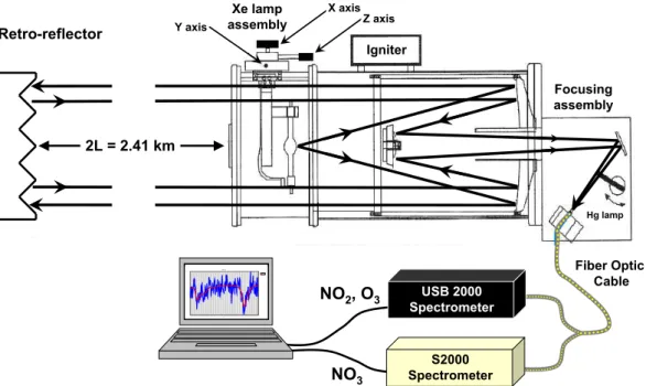
DOAS measurements were made using a modified DOAS 2000 Instrument (TEI Inc.), Fig. 2. The instrument utilizes a 150 W high pressure Xe-arc lamp and a coaxial

5

Cassegrain telescope. The outgoing beam is collimated by the outer portion of the 8′′primary telescope mirror. The beam traverses through the open atmosphere and is reflected from a retro reflector composed of 7×2′′ corner cube reflectors. The DOAS retro reflector was located on Tumbo Island (Fig. 1 inset) at an elevation of 6 m a.s.l. The total path length was 2407 km with the majority of the path (2.1 km) over the ocean

10

at a mean elevation of 15 m a.s.l. The return beam is focused by the inner portion of the primary mirror onto a modified detector system including a bifurcated quartz fiber optic (Ocean Optics) with dual 400µm fibers, each fiber leading to a different fiber optic spectrometer. One spectrometer was optimized for NO2 and UV absorption fea-tures (USB2000, Grating #10, 492 nm, 1800 lines mm−1, 2048 element CCD, 25µm slit,

15

UV2 upgrade, L2 lens) with optical resolution of∼0.5 nm; and one was optimized for NO3absorption in the red end of the visible spectrum (S2000,λblaze=750 nm, 840 nm, 1200 lines mm−1, 2048 element CCD, 25µm slit, L2 lens) with an optical resolution of ∼0.6 nm. A small diffuser was installed in the entrance end of the fiber to lower atmo-spheric turbulence noise (Stutz and Platt, 1997). The spectrometers were cooled to

20

−5◦C in a portable freezer.

For the NO3measurements (S2000), data was collected with OOIBase32 software. Typical integration times were 25–30 ms. Averages of 30 000 spectra were computed and streamed to disk, resulting in a time resolution of ca 8–15 min when visibility was good. For the NO2measurements (USB2000), custom acquisition software was

25

(10)

ACPD

9, 24531–24585, 2009

R. McLaren et al.

Title Page

Tables Figures

◭ ◮

Back Close

Full Screen / Esc

reference spectra were collected periodically for wavelength calibration and for con-voluting molecular reference spectra to the slit function of the spectrometer. Xenon lamp spectra were collected for use in fitting to the measured spectra. Each ambient spectrum was also corrected for electronic offset and dark noise.

The averaged spectra were fit using DOASIS software (Kraus, 2006). For NO₃,

typi-5

cal fit scenarios included a convoluted NO3reference spectrum (Yokelson et al., 1994), a convoluted water spectrum (Coheur et al., 2002), a Xe lamp spectrum in the region from 617–673 nm and a third order polynomial. It was found that better results were generally obtained by using an early evening or early morning ambient spectrum, at a time when NO3 is determined to be negligible, in place of a lamp reference

spec-10

trum (Platt, 1994). The presence of two strong absorption features at 623 and 662 nm were used to qualitatively identify the presence of NO3. For NO2, fit scenarios included a lamp reference spectrum, a convoluted spectrum of NO2 (Voigt et al., 2002) in the region from 422–437.5 nm and a third order polynomial. Independent studies using injections of high concentrations of a standard mixture of NO2in air into an absorption

15

cell positioned in the DOAS beam path confirmed that our DOASIS retrieval methods were accurate to within 10% for NO₂mixing ratios from 1–100 ppb. Detection limits for NO3and NO2were 4 ppt and 2 ppb respectively, taken as 2σin the residuals of the fit. Ozone was also measured by DOAS by fitting the nighttime spectra collected with the UV spectrometer in the region of 316.8–329.9 nm. The fit included a reference

20

spectrum for O3 (Bogumil et al., 2001), one for NO2, a Xe lamp spectrum and third order polynomial. This region is not the ideal region for measurement of O3by DOAS, as the differential absorption cross sections are relatively small. Despite this, O₃was measurable with uncertainties of±5 ppb simultaneously in the same path as NO2and NO3. This O3 data set was preferred compared to the use of the O3 measurements

25

from the CAPMon station 6 km away due to the observation of differences in NO₂ pollu-tant levels on the north and south sides of the island. Overall the average nighttime O3 levels at East Point were 5.5 ppb lower than those measured at the CAPMon station.

(11)

ACPD

9, 24531–24585, 2009

R. McLaren et al.

Title Page

Tables Figures

◭ ◮

Back Close

Full Screen / Esc

4 Results and Discussion

4.1 NO3, NO2and O3observations

Observations of NO₃and NO₂throughout the study are shown in Fig. 3. Measurements were made on 16 nights for NO2and O3, and 13 nights for NO3. Negative results are shown for completeness, and are expected to occur when levels are at, or below the

5

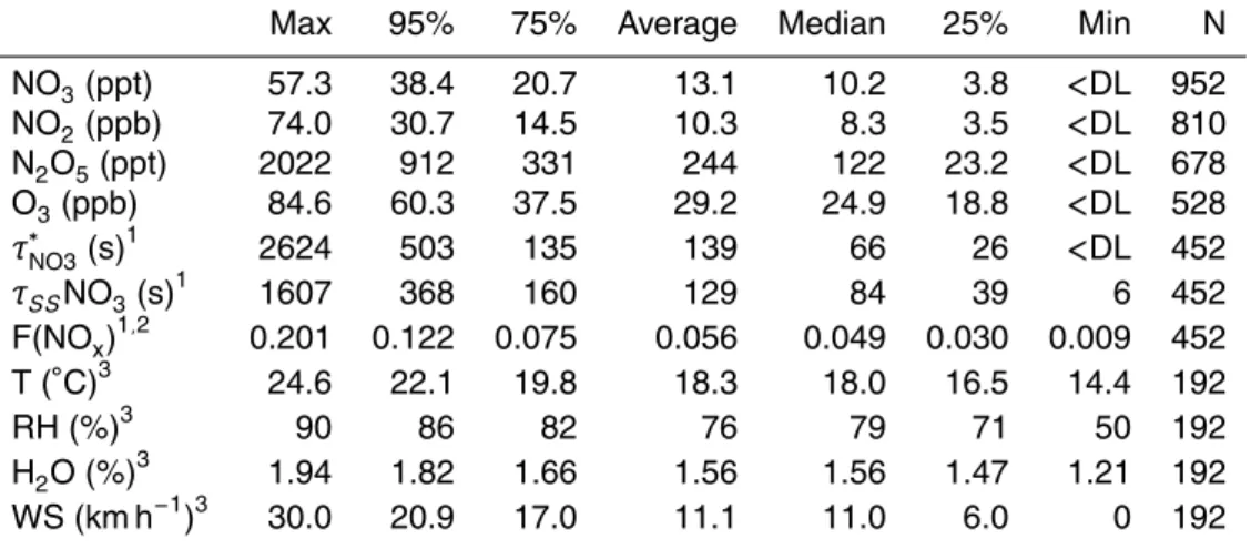
detection limit. A summary of statistics for the chemical observations of NO₃, NO₂ and O3 at night (between 08:00 p.m. and 08:00 a.m. PLT) are given in Table 1, along with other important meteorological observations that are relevant for formation and loss of NO₃and N₂O₅. Maximum mixing ratios of NO₃(8–15 min average) were above 20 ppt every night. The range of nightly maximum levels was 22–57 ppt, with an

av-10

erage nightly maximum level of 40.0 ppt, roughly consistent with the 95th percentile of all observations of 38 ppt. The average and median for all nighttime observations of NO3 were 13.1 ppt and 10.2 ppt respectively. Measurements of NO3 were not made during the day but are generally expected to be<1 ppt due to rapid loss by photoly-sis. Thus, median and average NO₃ mixing ratios relevant for 24 h periods would be

15

approximately half the values stated above, 5.1–6.5 ppt.

A nocturnal profile for NO3, based on 30 min time bins of all observations, is given in Fig. 4. The profile shows NO₃ increasing after sunset with a maximum between midnight and 1 a.m. (25th, 50th, 75th percentiles and average). NO3 slowly decays after that time until sunrise, when it approaches zero. The central values and range of

20

concentrations we report here are similar to values reported in summer time in other marine areas (Vrekoussis et al., 2007, and references within). Despite the higher NO2 levels in this region that would increase the production rate of NO3via Reaction (R1), the levels of NO₃are not necessarily higher than seen in other less polluted areas. This is due to the subsequent loss of NO3to form N2O5via Reaction (R2f), also proportional

25

to NO2, rendering NO3insensitive to NO2as a first approximation.

(12)

ACPD

9, 24531–24585, 2009

R. McLaren et al.

Title Page

Tables Figures

◭ ◮

Back Close

Full Screen / Esc

this, the nighttime median ozone levels at East Point were significantly higher than those observed at all monitoring stations in the LFV mainland, where the range was 1.0–18.5 ppb for 19 stations. Frequent titrations of ozone to zero are observed at the mainland stations at night, due to a combination of anthropogenic emissions of NOx from on-road vehicles in a shallow nocturnal inversion layer, and high rates of

deposi-5

tion over continental surfaces. Deposition velocities of ozone over water are known to be significantly smaller.

Nighttime levels of NO₂ at East Point were quite high for the MBL, as indicated in Fig. 3 and Table 1. Median and average nighttime levels were 8.3 ppb and 10.3 ppb respectively. These levels of NO2are much higher than those reported in many recent

10

studies of nighttime chemistry in the MBL (Allan et al., 2000; Martinez et al., 2000; Vrekoussis et al., 2004, 2007; Matsumoto et al., 2006). Although vehicular traffic is min-imal on the island, the proximity of Saturna Island to multiple populated regions gives rise to an overall elevated background level of NO_x in this marine region. Nocturnal build up of pollutants can occur in the Strait during stagnation events, due to the wake

15

induced stagnation effect (Brook et al., 2004). In addition, marine vessels are a major contributor to the total emissions of NO_xin the region, especially in the Strait of Geor-gia. A recent air pollutant emissions inventory of the LFV (Metro Vancouver, 2007), including mainland and marine regions, indicated that emissions of NOx from marine vessels were 8.4×106kg yr−1 in 2005 or 14% of the total anthropogenic NO_x

emis-20

sions, and are projected to rise in both absolute and relative terms to 13.6×106kg yr−1, and 30% respectively, by the year 2030. Most of these emissions are in the MBL in the western end of the domain (Fig. 1). Marine vessels destined for the Pacific Ocean leave Vancouver ports travelling south and generally follow a shipping lane that follows the Canada/USA border leading to the Strait of Juan de Fuca. This brings ocean going

25

vessels to within a few kilometers of East Point, frequently visible throughout the study. A comparison of the study average nocturnal pattern of NO₂ measured by DOAS, compared to that reported at a few representative monitoring stations in the LFV is shown in Fig. 5. The mixing ratios of NO2at Saturna are on the lower end of the range

(13)

ACPD

9, 24531–24585, 2009

R. McLaren et al.

Title Page

Tables Figures

◭ ◮

Back Close

Full Screen / Esc

observed in the Valley. The highest NO₂ levels are observed in the north western portion of the valley, close to the urban region of Vancouver. Station T1, in downtown Vancouver, experiences the highest NO2levels of all 19 reporting stations. The levels of NO₂ at East Point are similar to those seen at Station T27 (Langley, BC), a mid valley station 40 km away, 20 km inland from the coast. The nocturnal profile of NO2at

5

East Point shows maximum levels in the middle of the night, as do all stations in the valley, typical of continental urban areas. The mainland stations show early morning peaks typical of vehicular traffic that is absent in the East Point profile, confirming the absence of significant vehicular traffic at the site.

The levels of NO₂ measured at East Point were clearly much higher than those

10

simultaneously measured at the CAPMon station on Saturna island, separated by only 6 km (Fig. 5). There are several explanations for this. First, the East Point site is more representative of the conditions experienced in the MBL, being at the confluence of two main stretches of the Strait at the north east tip of the island. The Gulf Islands can act as a physical barrier to surface flow and as such, emissions from marine vessels

15

within the Strait and outflow (land breezes) from the LFV at night are likely confined to the Strait. Evidence for this lies within Figure 6c, which shows the frequency of wind directions observed at night when winds were not stagnant (>2 km h−1). There are two main wind sectors observed at East Point at night. The first is a 50◦ sector from 195– 245◦, which collectively accounts for 67% of all nighttime observations; here within

20

referred to as the southwest sector. The second sector, the northwest sector, from 285–335◦, accounts for 18% of observations. Collectively, these two sectors account for 85% of all non-stagnant observations, and are aligned with the main directions of the channels of the Strait of Georgia; NW-SE and SW-NE. The NW sector likely contains outflow emissions from Vancouver as well as marine vessel emissions, whereas the

25

SW sector likely contains emissions from Victoria as well as marine vessel emissions. Stagnant conditions were observed 2.6% of the time.

(14)

ACPD

9, 24531–24585, 2009

R. McLaren et al.

Title Page

Tables Figures

◭ ◮

Back Close

Full Screen / Esc

elevation. The CAPMon site is positioned inland at an elevation of 200±5 m. At night, the site is likely within a surface layer or nocturnal boundary layer (Brown et al., 2007) that is isolated and decoupled from the surrounding MBL. With few surface sources on the island, the NO₂ levels are low. Winds from the southwest sector approaching the CAPMon site encounter a physical barrier, a 400 m cliffat the west end of the island

5

gradually decreasing to 250 m directly south of the CAPMon site. This physical barrier perturbs surface marine flow, as mentioned previously, and likely further decouples the CAPMon site from surface emissions at night. In contrast, the East Point site has a measurement beam elevation of 15±9 m a.s.l. situated largely within the MBL. It is exposed to surface emissions within the MBL. In addition, vertical mixing over water in

10

the MBL will be slow, especially at night, and thus surface emissions over the water are likely stratified.

Figure 6 shows the dependence of the NO3and NO2observations on wind direction. In general NO₃ showed slightly elevated levels in the SW and NW sectors compared to the other observations. NO2 showed elevated levels when winds were from the

15

SE quadrant, however infrequently (7.3% of the time), and from the SW sector. It is worth noting that the SE quadrant is the quadrant that contains the closest approach of marine vessels to the tip of East Point, whereas the SW sector aligns with the shipping highways in the lower leg of the Strait of Georgia, Haro Strait, and the City of Victoria.

For the above reasons, we conclude that the site at East Point is representative of

20

a polluted MBL at night that is frequently impacted by emissions from marine vessels and from regional anthropogenic emissions from surrounding urban areas. The NO2 levels seen at night are similar to those observed in the less populated regions of the LFV.

4.2 N₂O₅and nighttime partitioning

25

N2O5 was calculated on a sample by sample basis from the known concentrations of NO₂and NO₃, along with use of the temperature dependant forward (Reaction R2f) and reverse rate constants (Reaction R2r) taken from recent recommendations (Atkinson

(15)

ACPD

9, 24531–24585, 2009

R. McLaren et al.

Title Page

Tables Figures

◭ ◮

Back Close

Full Screen / Esc

et al., 2004). Temperature data from the meteorological database was used for each coincident observation. Uncertainties in the N₂O₅levels have been calculated via prop-agation of uncertainties in the NO3 and NO2 values. There are also uncertainties in the forward and reverse rate constants, and hence, the corresponding equilibrium con-stant, K. Including a 10% uncertainty in each of the forward and reverse rate constants,

5

the overall relative uncertainty in the calculated N2O5levels for a single point is±24% at levels corresponding to the 95th percentile (∼900 ppt). In calculating N2O5, the as-sumption is that equilibrium exists between NO₂, NO₃ and N₂O₅. This is generally true under conditions of high temperatures and high NO2 that promote high turnover times of NO3and N2O5for Reactions (R2f) and (R2r) respectively. For example, using

10

the median overnight temperature of 18◦C, k_2r₌1.89×10−2s−1, giving a N₂O₅ lifetime with respect to thermal decomposition of 53 s. Correspondingly, at the same temper-ature, k2f=1.3×10−

12

cm3molec−1s−1, and in the presence of 8.3 ppb of NO2(median level), the lifetime of NO₃with respect to reaction with NO₂is 4 s. Thus, equilibrium is established very rapidly under these conditions.

15

Calculated N2O5mixing ratios had maximum values above 300 ppt every night, rang-ing from 369–2022 ppt with a median maximum nightly value of 928 ppt, roughly con-sistent with the 95th percentile of all nighttime observations of 912 ppt. Average and median levels over the course of the night were 244 ppt and 122 ppt respectively. These levels are much higher than typically reported for the summer MBL (Allan et al., 2000;

20

Vrekoussis et al., 2004; Matsumoto et al., 2006; Vrekoussis et al., 2007), primarily due to the focus of other studies on remote or only moderately polluted locations. On the edge of the Baltic Sea in summer, the occasional N₂O₅level up to 2 ppb during pollu-tion events was reported (Heintz et al., 1996). N2O5 levels of 1 ppb were reported in moderately polluted air offthe east coast of USA, with average N2O5 nighttime levels

25

(16)

ACPD

9, 24531–24585, 2009

R. McLaren et al.

Title Page

Tables Figures

◭ ◮

Back Close

Full Screen / Esc

N₂O₅/NO₃ratio of 16.8 and 13.1 respectively. This high ratio is a direct consequence of the high levels of NO2. For example, at 18

◦

C, the threshold mixing ratio of NO2 at which the N2O5/NO3 equilibrium ratio is unity is ∼0.6 ppb. When NO2 is below this level, the equilibrium N₂O₅mixing ratio is smaller than NO₃. For example, in the east-ern Mediterranean, average summer values of the N2O5/NO3ratio were 0.34±0.26 in

5

the presence of average NO2 levels less than 0.5 ppb (Vrekoussis et al., 2004). To contrast this, in moderately polluted air (average NO₂=4.0 ppb), the ratio of average N2O5 to average NO3 was 4.9 (Brown et al., 2004). An important consequence of high N2O5/NO3ratios in polluted air is the potential for increased importance of indirect losses of NO₃, via reactions of N₂O₅. This rationale was noted previously (Martinez

10

et al., 2000), and is supported by conclusions in a study of the remote MBL, namely that in remote marine air, losses of NO3were dominated by direct reactions with DMS, whereas in moderately polluted air, indirect losses of NO3 via N2O5 reactions usually dominated (Allan et al., 2000).

Apart from the [N2O5]/[NO3] ratio, an additional diagnostic parameter is the molar

15

partitioning of total oxidized nitrogen, NOy, that is attributable to nighttime reservoir species, NO₃ and N₂O₅ (Brown et al., 2003b; McLaren et al., 2004). A similar di-agnostic is the nocturnal partitioning, F(NOx), among the three equilibrium species in Reaction (R1),

F(NO_x)= [NO3]+2[N2O5]

[NO2]+[NO3]+2[N2O5]

(2)

20

F(NOx) is a measure of the proportion of nitrogen oxide stored in the nocturnal reser-voir of NO₃ and N₂O₅ (Brown et al., 2007). High values of F(NO_x) can be indicative of long lifetimes for NO3 and N2O5 and are expected to increase as temperature de-creases, whereas low values of nocturnal partitioning are expected when lifetimes of NO3and N2O5are small. In the current study, the values for F(NOx) ranged from zero

25

to 20% with average and median values of about 5%, Table 1. These are comparable to nocturnal partitioning of 5%, calculated from data within the report of the moderately

(17)

ACPD

9, 24531–24585, 2009

R. McLaren et al.

Title Page

Tables Figures

◭ ◮

Back Close

Full Screen / Esc

polluted summer MBL (Brown et al., 2004). The average nocturnal partitioning of 5% in the current study is also consistent with a recent report (Brown et al., 2007) in which F(NOx) was less than 10% in the continental nocturnal boundary layer, where short NO3 lifetimes suggested rapid sinks for NO3and N2O5, but F(NOx) increased rapidly with height above the nocturnal boundary layer, to F(NO_x)₌35%, coincident with a rapid

5

increase in the NO3lifetime with height.

4.3 Lifetime and losses of NO3

4.3.1 Theoretical aspects

A useful parameter to calculate is the lifetime of the NO₃radical,τNO3. An expression for the apparent lifetime of NO3 can be derived with knowledge of the known source

10

(Reaction R1), its reversible reaction to form N2O5(Reactions R2f, R2r), and indeter-minate losses of NO₃ and N₂O₅ such as those shown previously (e.g. Reactions R7, R8, R9, R10). The derivation has been presented previously (Martinez et al., 2000), with the main assumptions being that the system is in steady-state balance between sources and losses of NO₃ and N₂O₅, d[NO₃]/dt=d[N₂O₅]/dt=0, and that equilibrium

15

in the NO2-NO3-N2O5 system has been established. If such is the case, then the steady-state lifetime of NO3is defined by:

τSS(NO3)=

[NO₃]

k₁[O₃][NO₂] (3)

A recent report (Brown et al., 2003a) discusses in detail the difference between the assumptions of steady-state and equilibrium, and illustrates convincingly that although

20

equilibrium can be achieved very rapidly, the approach to steady-state can take much longer, on the order of several hours, especially under conditions of high NO2 and low temperatures. Lifetimes calculated using the steady-state approximation can be significantly biased in such cases, and the conclusions made from analysis of the life-times are cast in doubt. Considering the high levels of NO₂encountered in this study,

(18)

ACPD

9, 24531–24585, 2009

R. McLaren et al.

Title Page

Tables Figures

◭ ◮

Back Close

Full Screen / Esc

we found it prudent to calculate lifetimes of NO₃without invoking the steady-state as-sumption using a relatively easy approach, but not reported previously to the best of our knowledge. We assume that the equilibrium shown in Eq. (1) is valid, and use our previous argument of fast turnover times at warm temperatures encountered in the study as evidence that equilibrium is, in fact, achieved rapidly. To derive an expression

5

for the non steady-state lifetimes of NO3, we formally consider a combined reservoir of NO₃and N₂O₅, ([NO₃]+[N₂O₅]), that has both sources and losses. Chemical inter-changes between NO3 and N2O5 do not need to be considered, since a gain or loss of a molecule of NO3 also results in a gain or loss of a molecule of N2O5, for a null change in the reservoir. The continuity equation for the reservoir, ignoring fluxes, is:

10

d{[NO3]+[N2O5]}

dt =SNO3+N2O5−LNO3+N2O5 (4)

The only known source to the reservoir is the production of NO3via Reaction 1:

SNO3+N2O5=k1[O3][NO2] (5)

The losses from the reservoir will occur through external losses of NO3 or N2O5 that can be parameterized as pseudo first order losses:

15

LNO3₊N2O5=LNO3+LN2O5=kx[NO3]+ky[N2O5] (6) where k_x and k_y are the overall pseudo first order rate constants for NO₃ and N₂O₅ respectively. Combining Eqs. (4), (5) and (6) we obtain:

k₁[O₃][NO₂]−d[NO3] dt −

d[N₂O₅]

dt =kx[NO3]+ky[N2O5] (7)

The lifetime of NO3 can generally be defined as the ratio of the concentration of NO3

20

to the losses of NO₃, L_NO3:

τNO3= [NO3]

LNO3

(8)

(19)

ACPD

9, 24531–24585, 2009

R. McLaren et al.

Title Page

Tables Figures

◭ ◮

Back Close

Full Screen / Esc

For the combined reservoir, we can define the lifetime of NO3, τ

∗

NO3, including direct and indirect losses from the reservoir:

τ_NO3∗ = [NO3]

LNO3+N2O5

(9)

Substituting Eqs. (4) and (5) into Eq. (9) we get:

τ_NO3∗ = [NO3]

k1[O3][NO2]− d[NO₃]

dt − d[N₂O₅]

dt

(10)

5

Note thatτ∗_NO3=τSS(NO3) if d[NO3]/dt=d[N2O5]/dt=0. Equation (10) represents a way to calculate the apparent lifetime of NO3in the NO2-NO3-N2O5equilibrium system with-out assuming steady-state, if one has continuous measurement data for NO₃, O₃, NO₂, and N2O5. It is possible to find the derivatives, d[NO3]/dt and d[N2O5]/dt by calculating the rate of change of NO3 and N2O5with respect to time from the observational data.

10

If measurements of [N₂O₅] are not available, [N₂O₅] can be calculated from Eq. (1) if it can be shown that equilibrium is established. We have used this latter approach in the current study. The derivatives, d[NO3]/dt and d[N2O5]/dt, were calculated using a three point running slope in the continuous data set. This approach introduces more noise into the calculation of the NO3lifetime, but with the benefit of unbiased lifetimes. Other

15

lifetimes can be calculated for the reservoir depending on preference and application. One can define the lifetime of N₂O₅,τ_N2O5∗ , including direct and indirect losses of N₂O₅ from the reservoir:

τ_N2O5∗ = [N2O5]

LNO3+N2O5

(11)

In this paper, we focus on the non steady-state lifetime of NO₃, τ∗_NO3, as it allows

20

(20)

ACPD

9, 24531–24585, 2009

R. McLaren et al.

Title Page

Tables Figures

◭ ◮

Back Close

Full Screen / Esc

N₂O₅from the equilibrium system as shown below. Dividing Eq. (7) by [NO₃] we obtain

k₁[O₃][NO₂]−d[NO3]

dt − d[N₂O₅]

dt [NO3]

=k_x₊k_y[N2O5] [NO3]

(12)

or expressed slightly differently, we write

(τ∗_NO3)−1=k_x+k_y[N2O5] [NO3]

=k_x+k_yK_eq[NO₂] (13)

5

This is the same equation presented previously by others (Allan et al., 2000; Brown et al., 2003a), with the exception that we use inverse non steady-state lifetimes in-stead of inverse in-steady-state lifetimes. This expression allows the determination of the overall first order rate constants for loss of NO3 and N2O5, kx and ky, from the inter-cept and slope of a plot of (τ_NO3∗ )−1 versus Keq[NO2], or equivalently, (τ

∗

NO3)

−1

versus

10

[N2O5]/[NO3].

4.3.2 Observations of NO₃lifetime and losses

The observed distribution of NO3 lifetimes throughout the study calculated according to Eq. (10) and via Eq. (3) are given in Table 1. The median values are similar, between 1–1.5 min, although there are di_fferences at the extremes of the distribution between

15

steady-state and non steady-state predictions. The temporal variation of lifetimes cal-culated using the two methods are shown in Fig. 7. Surprisingly, the nocturnal patterns look similar although there are subtle di_fferences. During periods when the nocturnal pool of NO3and N2O5is building such as early evening, d[NO3]/dt and d[N2O5]/dt are positive, and we would expect the steady-state assumption to predict lifetimes that are

20

shorter than the true lifetime. This is true on average before midnight using the data

(21)

ACPD

9, 24531–24585, 2009

R. McLaren et al.

Title Page

Tables Figures

◭ ◮

Back Close

Full Screen / Esc

seen in Fig. 7, although only marginally so. The reverse would be true during periods when the nighttime reservoir pool is depleting rapidly; d[N₂O₅]/dt and d[NO₃]/dt are negative and the steady-state lifetime is expected to be larger than the true lifetime. This trend is somewhat more obvious in Fig. 7, perhaps due to the lower temperatures during the latter part of the night that slow the kinetics and the approach to

steady-5

state. It is likely that overall, the relatively warm nighttime temperatures encountered in this study (Table 1) assist in a more rapid approach to steady-state than encountered in the previous modeling study by Brown (2003; 12◦C), where the differences between τSS(NO3) and (kNO3)

−1

were more obvious. For example, the thermal decomposition of N2O5 (Reaction R2r), has a rate of reaction that more than doubles by increasing the

10

temperature from 12◦C to 18◦C. The median and average NO₃ lifetimes of 1–1.5 min and 2–2.5 min calculated here can be compared to other studies in the MBL;∼4.2 min annual average in the Baltic sea (Heintz et al., 1996),∼3 min in the summer Mediter-ranean (Vrekoussis et al., 2004), between 1 and 20 min in the north east and central east Atlantic (Allan et al., 2000), and between 0.2 to 17 min in a coastal region off

Ger-15

many (Martinez et al., 2000). A general observation in the above studies is that the lowest lifetimes are observed under the influence of polluted air masses. Our results are consistent with this.

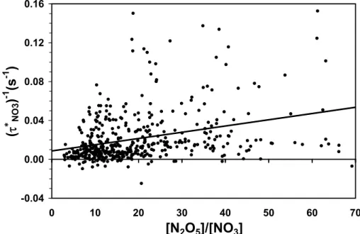
Regression of (τ_NO3∗ )−1 with [N2O5]/[NO2] for all nighttime data is shown in Fig. 8. The r2 for the regression is only 0.10, implying that only 10% of the variance can

20

be accounted for by the correlation with [N2O5]/[NO3]. Nonetheless, as suggested by Eq. (13), the intercept and slope provide overall first order rate constants for loss of NO₃ and N2O5respectively: kx=0.0087±0.0020 s−

1

, ky=5.72(±0.81)×10− 4

s−1. These can at best be interpreted as average rate constants encountered for the entire study, as undoubtedly, the rate constants would vary depending on many parameters including

25

(22)

ACPD

9, 24531–24585, 2009

R. McLaren et al.

Title Page

Tables Figures

◭ ◮

Back Close

Full Screen / Esc

[N₂O₅]/[NO₃]=15 (median =13.1, average=16.8), we determine that 50.4±13.2% of losses of NO3 are direct, compared to 49.6±9.6% of losses that are indirect through losses of N2O5.

One approach to remove much of the variability in the previous methodology is to an-alyze subsets of the data according to time bins. The rationale is that many parameters

5

follow general trend patterns during the night; temperature decreases, relative humidity increases, wind speeds decrease, reactive VOCs decrease, to name a few. Figure 9 shows the results of such an analysis in which hourly binned data from the study are regressed according to Eq. (9) to determine the nocturnal pattern in kxand ky. As can be seen, a dramatic decrease in the value of k_x occurs in the first few hours of the

10

night, to values that are zero within statistical error. Ignoring photolysis and the slow heterogeneous loss of NO3, the value of kx at night would be given by the following equation:

kx=kNONO3[NO]+ X

i

ki,NO3[VOC]i (14)

where kNONO3is the rate constant for the reaction of NO3with NO and ki,NO3is the rate

15

constant for reaction of NO₃with an individual VOC_i. As no ancillary measurements of NO or VOCs were made at the location, we cannot confirm the magnitude of the direct sink of NO3 from these reactions, although it is known that the region is influenced by NO_x emissions from ship plumes (Lu et al., 2006), large fluxes of DMS (Sharma et al., 2003),α-pinene (McLaren et al., 2004), isoprene and a range of anthropogenic

20

VOCs (Jiang et al., 1997). Temporal profiles in the MBL in other regions indicate that rapid depletion of DMS due to reaction with NO₃occurs during the first few hours after sunset (Vrekoussis et al., 2004). Depletions of monoterpenes and isoprene by NO3 after sunset are also known to occur in continental areas (Geyer et al., 2001; Brown et al., 2009), as are certain reactive anthropogenic hydrocarbons (Dimitroulopoulou

25

and Marsh, 1997). Using rate constants for the reaction of NO3 with VOCs (Atkin-son et al., 2004, 2006), the value of kx observed early in the evening (kx=0.034 s−

(23)

ACPD

9, 24531–24585, 2009

R. McLaren et al.

Title Page

Tables Figures

◭ ◮

Back Close

Full Screen / Esc

would be consistent with individual reactions of NO₃ with 52 ppt of NO, 1.2 ppb DMS, 1.9 ppb isoprene, 219 pptα-pinene, 4.0 ppb i-butene,∼100 ppt of any isomer of cresol, or an appropriate mixture of the above. The summer time flux of DMS from the Strait of Georgia has recently been estimated to be 2.2µmol m−2day−1 (Sharma et al., 2003). Using this flux and assumptions of a boundary marine layer height of 100 m,

5

[OH]=2.5×106molec cm−3 during day, [NO3]=2.5×10 8

molec cm−3 (10 ppt) at night, k_OH_,_DMS=6.5×10−12molec−1cm3s−1 , k_NO3_,_DMS=1.1×10−12molec−1cm3s−1, a simple box model analysis predicts a daytime concentration of DMS that builds to 200 ppt at sunset, followed by a rapid decline over a few hours to a steady-state value of 22 ppt in the latter parts of the night. Combining this information with the early night value of

10

kxleads us to conclude that DMS is not the main sink for NO3in the early evening, al-though NO3is likely the main sink for DMS. Further study with ancillary measurements of VOCs would be needed to confirm the magnitude of the direct sink for NO₃reported here, and to determine the relative contribution of each hydrocarbon.

The value of ky observed in Fig. 9 is roughly constant for the first few hours of the

15

night and then increases in the latter parts of the night. Losses of N₂O₅ are known to occur through homogeneous reactions with H2O (Reaction R10), with the current recommendation (Atkinson, 2004) of both a first order and second order dependence on H₂O based upon recent work (Wahner et al., 1998), and through heterogeneous reactions on the surface of aerosols to produce HNO3 (Reaction R9), ClNO2

(Reac-20

tion R11) and Cl2(Reaction R12). The overall pseudo first order rate constant for loss of N2O5, ky, could be expressed as:

ky=khomo+khet=k10a[H2O]+k10b[H2O]2+ γA

4 r

8RT

πM (15)

where k10a=2.5×10

−22

cm3molecule−1s−1, k10b=1.8×10

−39

cm6molecule−2s−1, γ is the uptake coefficient of N2O5on the aerosol, A is the surface area of the aerosol, R is

25

(24)

ACPD

9, 24531–24585, 2009

R. McLaren et al.

Title Page

Tables Figures

◭ ◮

Back Close

Full Screen / Esc

Eq. (15), was calculated for all observations and has been plotted in Fig. 9 as the dot-ted line. The last term in Eq. (15) is equivalent to the rate constant for heterogeneous reactions of N2O5on aerosols, khet, a simplification of the Fuchs and Sutugin equation (Fuchs and Sutugin, 1971) forγ<0.1. Without ancillary measurements of aerosol sur-face area at the site, we cannot directly determine the magnitude of the last term in

5

(Reaction R15), although we can estimate it by difference.

The magnitude of the observed ky is consistent with the homogeneous gas phase hydrolysis of N₂O₅, k_homo, during the first few hours after sunset. The value of k_y in-creases after 2 am to values that are statistically greater than khomo, indicating that het-erogeneous reactions of N2O5 on aerosols become more significant at this time. The

10

average relative humidity at Saturna increased from∼68% just after sunset to a max-imum of 82% just before sunrise. The timing of the increase in ky at 1–2 a.m. roughly corresponds to the time when the relative humidity increases beyond the deliques-cence relative humidity (DRH) point for sea salt aerosols, 75%. This may indicate that the marine air mass contains dry sea salt aerosols or possibly other types of

15

dry aerosols. It seems unlikely that the MBL would contain locally generated dry sea salt aerosols as the lowest relative humidity observed throughout the study, was 46%, which is greater than the efflorescence relative humidity (ERH) of sea salt, 43±3%, the RH we expect is needed for sea salt spray to produce dry aerosols. It is possible that the MBL contains crystalline sea salt aerosols through other mechanisms such as

20

mixing of marine air with dry air through subsidence, or for the marine air mass to have part of its back trajectory over drier terrestrial regions. The latter could be accomplished through classic sea/land breeze recirculation during the day/night that is well charac-terized in this region (Hedley and Singleton, 1997). In another study (Vrekoussis et al., 2007), it was observed that the correlation between ln(τNO3) and ln(NO2), became

25

more negative as RH increased, taken as evidence that supports the existence of in-direct sinks of NO3that are related to the presence of water vapor in the atmosphere. We note that while RH increases through the night, the absolute concentration of water is roughly constant, or actually decreases slightly as the night progresses. As such, the

(25)

ACPD

9, 24531–24585, 2009

R. McLaren et al.

Title Page

Tables Figures

◭ ◮

Back Close

Full Screen / Esc

results presented here strongly suggest that the increased indirect sinks of NO₃ with increasing relative humidity are not related to the homogeneous loss of N2O5, but are related to the heterogeneous loss of N2O5. However, we also observe that the losses of N₂O₅ via the homogeneous hydrolysis mechanism are not insignificant, ranging in this study from up to 100% early in the night to a minimum of 23% later in the night,

al-5

though this should be tempered by the uncertain nature of the current recommendation for the homogeneous rate constant of N₂O₅with H₂O.

The values of ky observed here, ranging from zero (within error), to∼1.6×10

−3 s−1, are within the range of values of (τN2O5)

−1

reported in other studies of calculated N₂O₅ in the MBL (Heintz et al., 1996; Martinez et al., 2000). Subtracting khomo from ky

10

(see Eq. 15), we obtain an estimate of khet, which ranges from zero (within error) in the first part of the night to a maximum of 1.2×10−3s−1 in the latter part of the night. In the polluted subtropical MBL, Osthoff et al. (2008) modeled their observations of NOx, NO3, N2O5, ClNO2 and O3 in order to estimate the magnitude of the overall loss of N₂O₅, included a heterogeneous reaction of N₂O₅ that produces just HNO₃,

15

and another heterogeneous reaction that produces HNO3 and ClNO2. The observed values of the combined loss coefficient of N2O5 for two case studies they presented were 3×10−3s−1 and 1.0×10−3s−1. The maximum values of k_yobserved in Fig. 9 are within the range simulated by Osthoffet al. (2008).

4.4 Relationship between nighttime chemistry and O₃ formation in the Lower

20

Fraser Valley

To look for a link between nighttime chemistry in the MBL of the Strait of Georgia and ozone formation in the LFV, we performed a semi-observational analysis using observational data of ozone at multiple monitoring stations in the valley and correlating these with overnight integrated concentrations of N₂O₅at Saturna. A brief description

25

(26)

ACPD

9, 24531–24585, 2009

R. McLaren et al.

Title Page

Tables Figures

◭ ◮

Back Close

Full Screen / Esc

The potential products in the heterogeneous and homogeneous reactions of N₂O₅ are HNO3, ClNO2, Cl2, and potentially others.

N2O5

sea salt aerosols

−−−−−−−−−−−−−→HNO3,ClNO2,Cl2,others (R15)

The production rate of a product Pi, from one of these reactions is given by:

dP_i

dt =khet,i[N2O5] (16)

5

The value of the individual pseudo first order rate constants, khet,iare uncertain and are a current source of research interest at this time. For photolabile species such as ClNO₂, and Cl₂ that have few losses at night, accumulation will occur overnight such that the total accumulated concentration by morning, Pi (t), assuming constant conditions and no losses, is given by:

10

P_i(t)=

t Z

0

k_het_,_i[N₂O₅]dt=k_het_,_i t Z

0

[N₂O₅]dt (17)

Production stops in the morning due to the short lifetime of NO3and N2O5during sunlit hours. It can be seen that the accumulated concentration is proportional to the integral of the N₂O₅ concentration with respect to time overnight, and proportional to the het-erogeneous rate constant that describes the rate of formation of Pi from N2O5. Here

15

we will make the assumption that the overnight integrated concentration of N2O5 at East Point is representative of the general conditions that occur in the MBL of the Strait overnight, and that the overnight integral of N2O5can be used as a surrogate for the amount of accumulated photolabile species each morning, without knowledge of the individual heterogeneous rate constants, k_het_,_i. The overnight integral was calculated

20

(27)

ACPD

9, 24531–24585, 2009

R. McLaren et al.

Title Page

Tables Figures

◭ ◮

Back Close

Full Screen / Esc

for each night using a summation over the N observations:

t

Z

0

[N2O5]dt= N X

j=1

[N2O5]j×(tend,j−tstart,j) (18)

where tend,jand tstart,jare the end and start times of the j-th observation. The overnight N₂O₅ integral at East Point ranged from 6.7×1013 to 4.9×1014molecules cm−3s, or 0.061–0.444 ppb-nights, where the unit “night” is defined in this context as a 12.0 h

5

overnight period.

Before going further, it is interesting to estimate how much ClNO₂ could be pro-duced on such nights in the presence of sea salt aerosol. Using a lower end het-erogeneous rate constant for the production of ClNO2from a recent study (Osthoffet al., 2008), k_het_,_ClNO2=1.0×10−4s−1, we calculate potential ClNO₂accumulations

rang-10

ing from 0.26–1.9 ppb over the course of thirteen nights, with a median amount of 0.73 ppb. The question of Cl− availability in the marine aerosol to produce such levels of ClNO₂arises. To answer this question, we have analysed data from a previous study (Anlauf et al., 2006) in the LFV where size segregated aerosol ionic composition was measured at several stations over the course of several weeks. Using 90th to 100th

15

percentiles of the total Na+ composition in aerosols measured at Langley and Slocan (close to T27 and T4, Fig. 1) as representing diluted marine air, and applying a Cl/Na molar ratio of 1.17 in sea water (Seinfeld and Pandis, 2006), we estimate that the Cl− content of the marine aerosol in the Strait contains minimum levels of 0.8–1.3 ppbV chloride, expressed as a gas mixing ratio for suitable comparison. Measured

accumu-20

lations higher than this would need to invoke other mechanisms of ClNO2 formation such as uptake of HCl on Cl− deficient sea salt aerosols (Osthoffet al., 2008), or the more recent report of heterogeneous reactions of N2O5 and HCl on surfaces (Raffet al., 2009).

Another approach we could use to estimate the overnight accumulation of ClNO2is

25

(28)

ACPD

9, 24531–24585, 2009

R. McLaren et al.

Title Page

Tables Figures

◭ ◮

Back Close

Full Screen / Esc

from Osthoff et al. (2008) that 11–61% of the source of the nighttime NO₃/N₂O₅ reservoir, namely Reaction (R1), is converted to ClNO2. They used the lower estimate of 10% and a modified reaction as a source of ClNO2 in their model, NO₂+O₃→0.9 NO3+0.1 ClNO2+O2. In a similar way, and using a lower limit conver-sion of 11% from Osthoff et al. (2008), we calculated ClNO2 accumulations from the

5

integral,

ClNO2(t)=0.11 t Z

0

k1[NO2][O3]dt (19)

Using this second approach, we calculated overnight ClNO2 accumulations ranging from 0.31–1.6 ppb, with a median amount of 0.77 ppb, similar to the estimate by the first method. Nevertheless, the first method is more desirable since it is directly linked

10

to the reactant N2O5, and would not suffer from cases of strong direct losses of NO3in the marine boundary layer that do not lead to production of ClNO₂. Both methods for estimating ClNO2accumulations suffer from very uncertain observational parameters, either the heterogeneous rate constant to produce ClNO2 or the overall conversion e_fficiency. Hence in the methodology to follow, we examine links to ozone formation

15

using overnight integrals of N2O5.

The effect, if any, of overnight accumulated photolabile species will be experienced in the LFV the next day only if there is transport of marine air from the Strait into the valley. Meteorological observational data from 6 stations (see Fig. 1) in the valley were examined to look for evidence of a sea breeze each day. A sea breeze in this region

20

has been identified similar to that of others (Snyder and Strawbridge, 2004), through examination of the wind direction (WD) vectors:

Inflow (sea breeze)≡180◦<WD<330◦ (20)

Outflow (land breeze)≡0◦<WD<120◦

To assess transport of marine air from the Strait into the LFV, a simple criterion

25

(29)

ACPD

9, 24531–24585, 2009

R. McLaren et al.

Title Page

Tables Figures

◭ ◮

Back Close

Full Screen / Esc

speeds >5 km h−1, at all 6 stations the following day. Considering 13 nights when overnight integrals of N2O5 were available, sea breezes were observed on 9 of the days that followed, with 4 of the days showing either no evidence or only partial evidence of a sea breeze. The 9 nights retained for subsequent analysis included 24/25 June, 25/26, 26/27, 27/28, 31 July, 1/2, 3/4, 5/6 and 6/7 August. The

aver-5

age wind vectors for afternoon hours on the 9 days when the sea breeze was well developed (12–4 p.m.) were: Vancouver International (WD=286◦, WS=17.6 km h−1), Sandheads (WD=287◦, WS=17.3 km h−1), Pitt Meadows (WD=258◦, WS=7.8 km h−1), White Rock (WD₌228◦, WS₌6.8 km h−1), Abbotsford (WD₌229◦, WS₌11.6 km h−1) and Hope (WD=290◦, WS=19.9 km h−1). A general observation of the

meteorologi-10

cal analysis is that sea breezes start and finish earlier for those stations close to the coast, compared to those stations further inland (i.e. Abbotsford and Hope). It should also be mentioned that there is evidence from previous studies in this area that sea salt aerosols are carried by the sea breeze very far inland, further than Abbotsford. These aerosols show classic Cl− deficiency compared to Na+due to heterogeneous reaction

15

with N2O5at night and/or HNO3displacement reactions during the day (McLaren et al., 2004; Anlauf et al., 2006).

In the semi-observational approach, regression analysis was performed separately for each monitoring station in the domain. Regression analysis was performed be-tween the maximum 1-h average O3 values at a station on the day following each

20

overnight period and the corresponding overnight N₂O₅ integrals, our surrogate for nighttime chemistry and accumulated amount of photolabile species. An example of the regressions for a few representative stations is given in Fig. 10. Linear regres-sion analysis was used to determine the slope of the relationship, dO₃/d∫[N2O5]dt. A zero slope indicates no effect (null hypothesis) while a positive slope of statistical

25