doi:10.5194/ars-13-169-2015
© Author(s) 2015. CC Attribution 3.0 License.
Fast algorithm for radio propagation modeling in realistic 3-D
urban environment
A. Rauch, J. Lianghai, A. Klein, and H. D. Schotten
University of Kaiserslautern, Paul-Ehrlich-Straße 11, 67663 Kaiserslautern, Germany Correspondence to:J. Lianghai ([email protected])
Received: 15 December 2014 – Revised: 6 April 2015 – Accepted: 26 April 2015 – Published: 3 November 2015
Abstract.Next generation wireless communication systems will consist of a large number of mobile or static terminals and should be able to fulfill multiple requirements depend-ing on the current situation. Low latency and high packet success transmission rates should be mentioned in this con-text and can be summarized as ultra-reliable communications (URC). Especially for domains like mobile gaming, mobile video services but also for security relevant scenarios like traffic safety, traffic control systems and emergency manage-ment URC will be more and more required to guarantee a working communication between the terminals all the time.
1 Introduction
In order to evaluate the performance of next generation mo-bile communication systems in realistic deployment scenar-ios, system level simulation tools must be capable of inte-grating various models that reflect network deployment (e.g., antenna locations, elevation, orientation, transmit powers), user mobility and communication behavior, as well as ser-vice characteristics. The need for modeling system aspects and use cases of next generation mobile networks in a more realistic manner system is already acknowledged by Euro-pean 5G research project ICT-317669 METIS (2013). In this paper we present a fast method for computing the path loss of micro and macro cells in a realistic, three dimensional ur-ban environment scenario for moving and stationary users. Therefore, we use a simplified recursive ray tracing algo-rithm, which only takes into account one ray for each user per base station. Channel fading will be simulated by using Rayleigh and Rician distributed fading. To achieve a realistic Rician distributed fading, we use a variablek factor that is randomly created taking into account the respective distance
between transmitter and receiver. Both Rayleigh and Rician fading will be precomputed for the correspondent situations and just added to the path loss to achieve shorter computa-tion times. Further, it is demonstrated that the employed al-gorithm is able to outperform the state-of-the-art approach described in Sect. 2.
The remainder of this paper is organized as follows: in Sect. 2 we give a short overview about the scenario layout and the user mobility. In Sect. 3 we present the path loss mod-els and discuss the commonly used parameters. The compu-tation of fast fading is presented in Sect. 4 while the simula-tion results are shown in Sect. 5.
2 Urban environment and user mobility 2.1 3-D Scenario
The three-dimensional scenario used in this paper is defined in ICT-317669 METIS (2013) and is called Madrid Grid sce-nario. This scenario consists of 15 buildings with different heights, one park area and corresponding streets between the buildings. The size of the scenario is 387 by 552 m. An overview about the scenario is given in Fig. 1.
As shown in Fig. 1, there are 13 base stations considered namely 12 microcells (yellow) and one macrocell (red). The carrier frequency is 2.6 GHz and 10 MHz have been chosen as the system bandwidth.
Each road consists of two lanes for driving and two park-ing lanes. The road called “Gran Via” exhibits three lanes for driving in each direction has no parking lanes.
2.2 User mobility
BS0
BS3 BS4
BS7 BS8
BS 11
BS 12
Figure 1. Madrid grid layout according to ICT-317669 METIS (2013).
same constant speed of 50 kmph. Changing directions is only possible at crossroads. The probability of a right or left turn is 25 % respectively, while the probability of moving straight ahead is 50 % at each crossroad.
3 Path loss models
3.1 Computation of macrocell path loss
In order to determine the path loss of macro cells, which are usually installed on rooftops, we use a path loss model that is proposed in ICT-317669 METIS (2013). This model takes into account the diffraction effects that radio signals experi-ence and that is responsible for most of the signal energy re-ceived on ground level in urban environments. In this model, the calculation is divided in two parts. The first partLfs de-scribes the free space loss of signal from transmit antenna to the edge of the rooftop (dr) and can be calculated as:
Lfs= −10log10
λ
4π dr 2
. (1)
The second part describes the diffraction loss of the signal from the rooftop to the receiver on street and is calculated as shown in Eq. (2).
Lrts= −10log10 h λ
2π2r 1
2− 1 2π+2
i
, (2)
where 2=tan−1
1h
x
,
and
r=p(1h)2+x2,
1hrepresents the difference of the building height and the mobile antenna height andxthe horizontal distance between the diffracting edge and the user. The resulting path loss is calculated as:
L=Lfs+Lrts. (3)
Further details related to this model are shown in ICT-317669 METIS (2013).
3.2 Computation of microcell path loss
In case of micro cells, which are installed below rooftop level in an urban environment, most of the signal energy reaches the user due to reflection between buildings, if the user is not in line of sight (LoS). Since tracing multiple signal re-flections is computionally expensive, we choose two separate models to compute the overall microcell path loss.
The first model is used, if the user is in line of sight and the path loss is calculated as shown in is shown in Eq. (4). LdB= −10log10
λ
4π d
,2, (4)
whereλ is the wavelength and d is the distance between transmitter and receiver.
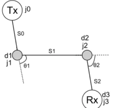
The second model is employed when the user is not in line of sight (nLoS). Here, we use Berg’s recursive path loss model (Berg, 1995), which takes into account geometrical conditions, such as angle of crossroads and distance between two crossroads. In principle, an imaginary distance is calcu-lated that depends on the real distances between transmitter and receiver and the angle between two streets.
Figure 3.Calculated path loss for moving user.
the considered dense urban scenario angle21and22are set to 90◦.
The imaginary distances are calculated according to Eq. (5) as described in Berg (1995).
kj=kj−1+dj−1qj−1,
dj=kj sj−1+dj−1, (5)
wherek0=1 andd0=0. The variableqrepresents the angle dependence of the path loss according to Eq. (6).
qj=
2j q90
90 v
. (6)
In this case,q90 is set to 0.5 andvis set to 1.5 as recom-mended in Berg (1995). The path loss is now calculated as follows:
L(n)dB = −10log10
λ
4π dn 2
, (7)
where dn is the imaginary distance between the respective transmitter and pointn.
Figure 3 shows the corresponding path loss characteris-tic of a user moving with constant speed from point P0 to point P2 in Fig. 4. The dotted line shows the path loss of the reference model, which is further described in ICT-317669 METIS (2013) and ITU-R M.2135 (2009). The continuous line depicts the path loss of the bergs model, that is used in our approach. This approach leads to a smoother curve that may be adjusted by using the parametersvandq90in Eq. (6). The corresponding base station is depicted in yellow in Fig. 4 as well.
As illustrated in Fig. 4 the user is in line of sight of BS4 until he reaches P2. After turning left, the user is in nLoS and the corresponding path loss model for a 90◦crossroad is chosen.
Fading is not considered here.
4 Computation of fast fading
Simulating fast fading in detail according to the three di-mensional scenario including multipath propagation due to
Figure 4.Movement of user.
reflection, diffraction and scattering would lead to a com-plex model that could not be computed in reasonable time. Since we simulate numerous moving users, the fast fading will be calculated by using some statistical approaches. As suggested in Tang and Hongbo (2003), Rayleigh and Rician distributions are used to generate fast fading. In the following sections, the utilization of both models is described.
4.1 Rayleigh distributed fast fading
If there is no dominant propagation path between transmit-ter and receiver (no line of sight) Rayleigh distributed ran-dom variables are used to describe fast fading, according to Eq. (8).
PRayleigh(r)= r
σ2 e −r2
2σ2, (8)
whereσ2represents the energy of the signal andrthe magni-tude. To calculate the Doppler power spectral density, we use Eq. (9), which is proposed in Kostov (2003), for the Rayleigh and Rician channel:
S(f )= 1
π fm r
1−
f fm
2, (9)
wherefmis the Doppler frequency shift that is calculated as: fm=
vfc
c , (10)
v=50 kmph represents the user speed,fcis the carrier fre-quency, which is 2.6 GHz in this case andc=3×10⁸m s−1 is the speed of light. The Rayleigh fading will be pre-calculated, stored and simply added to the path loss during the simulation.
4.2 Rician distributed fast fading
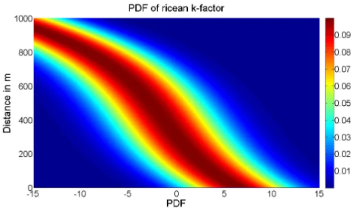
Figure 5.PDF of the riceankfactor.
Rician distributed random variables. Rician distributed fast fading can be described as:
PRice(r)= r σ2 e
−r2
2σ2+KI0
hrβ
σ2 i
,∀r≥0 (11)
withK= β2
2σ2 (Jeruchim et al., 2000; Iskander, 2008). For K=0 and I0
h rβ σ2 i
=1 Eq. (11) leads again to the Rayleigh fading calculated in Eq. (8) as proposed in Kostov (2003). The variableK is called Riceankfactor and rather describes the relation between the signal of the line of sight path and the non line of sight paths. As proposed in Thiele et al. (2006), the non line of sight signal components need to be summed up to determine thekfactor. To avoid simulating every single signal path we use the statistical approaches to estimate thekfactor, that are described in Thiele et al. (2006), Medawar et al. (2013) and Greenstein et al. (1999). In Thiele et al. (2006) and Medawar et al. (2013) functions are pro-vided that take into account the urban environment and the distance between transmitter and receiver resulting in a cu-mulative distribution function (CDF) of the Riciankfactor.
Thekfactor is now calculated using the line of sight dis-tance from transmitter to receiver and a random value, which is generated according to the corresponding probability dis-tribution function. Figure 5 shows the probability disdis-tribution function (PDF) of thek factor over the distance, where the y axis represents the distance in meters, thezaxis stands for the probability, and thexaxis shows thekfactor in dB.
As shown in Fig. 5, the probability of a highkfactor value decreases with an increasing distance between receiver and transmitter. In our simulation tool the k factor values are stored separately and used to generate Rician fading for the relevant distance between transmitter and receiver according to Eq. (11) (Jeruchim et al., 2000; Iskander, 2008).
Figures 6 and 7 show the fast fading for akfactor of 0 and 15 dB respectively.
Fork=0 the Ricean fading transfers into Rayleigh fading as shown in Eqs. (11) and (8).
Figure 6.Ricean fading fork=0 dB.
Figure 7.Ricean fading fork=15 dB.
5 Simulation results
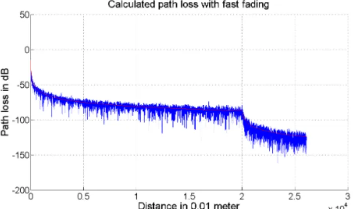
In this section, we will present some simulation results re-garding the path loss of a moving user in the described sce-nario. Figure 8 shows the path loss between transmitter and a moving user that follows the same route as described in Fig. 4. The Riciankfactor for nLoS conditions changes due to the distance as shown in Fig. 5. The appropriate models for fading and propagation will be chosen automatically using a single ray to detect NLoS or LoS conditions. The simulated path loss from P0 to P2 is shown in Fig. 8.
Figure 8.Path loss with fast fading.
Figure 9.Refresh rate vs. number of users.
As illustrated in Fig. 9 we can simulate up to 80 more users with the method proposed in this paper at a frame refresh rate of 30 fps than with the reference method.
6 Conclusions
In this work, we use a simplified model for efficiently com-puting the path loss between receiver and transmitter in line of sight conditions as well as in non line of sight conditions using Berg’s recursive model. To achieve realistic simulation results we combine this model with fast fading models, such as Rayleigh distributed fading for non line of sight propaga-tion. To consider multipath fading in line of sight conditions, we employ Rician distributed fading with a variablekfactor, which depends on the distance between transmitter and re-ceiver. The proposed model was compared with a reference model that does not use pre-computation and recursive algo-rithms. The model presented in this paper leads to a better performance that allows to simulate more moving users in a realistic 3-D-environment.
Acknowledgements. Part of this work has been performed in the framework of the FP7 project ICT-317669 METIS – Mobile and wireless communications Enablers for the 2020 Information Society, which is partly funded by the European Commission. This paper expresses the authors views, which are not necessarily those of the METIS consortium. The authors alone are responsible for the content of this paper.
Edited by: M. Chandra
Reviewed by: two anonymous referees
References
Berg, J.-E.: A Recursive Method For Street Microcell Path Loss Calculation, Proc. IEEE International Symposium on Personal, Indoor and Mobile Radio Communications, 1, 140–143, 1995. Greenstein, L., Michelson, D., and Erceg, V.: Moment-Method
Es-timation of the Rician K-Factor, IEEE Comm. Lett., 3, 175–176, doi:10.1109/4234.769521, 1999.
ICT-317669 METIS: Deliverable 6.1, ICT-317669, available at https://www.metis2020.com, 2013.
Iskander, C.-D.: A MATLAB-based Object-Oriented Approach to Multipath Fading Channel Simulation, white paper, February 2008.
ITU-R M.2135: Guidelines for evaluation of radio inter-face technologies for IMT-Advanced, M.2135, available at: https://www.itu.int/dms_pub/itu-r/opb/rep/R-REP-M. 2135-1-2009-PDF-E.pdf, 2009.
Jeruchim, M. C., Balaban, P., and Shanmugan, K. S.: Simulation of Communication Systems, 2nd Edn., New York, Kluwer Aca-demic/Plenum, 2000.
Kostov, N.: Mobile Radio Channels Modeling in MATLAB, De-partment of Radio Engineering, Technical University of Varna, RadioEngineering, 12, 12–16, 2003.
Medawar, S., Haendel, P., and Zetterberg, P: Approximate Maxi-mum Likelihood Estimation of Rician K-Factor and Investiga-tion of Urban Wireless Measurements, Trans. Wireless Comm., 12, 2545–2555, doi:10.1109/TWC.2013.042413.111734, 2013. Saunders, S. R.: Antennas and propagation for wireless
communi-cation systems, John Wily & Sons, Ltd., New York, 1999. Tang, L. and Hongbo, Z.: Analysis and Simulation of Nakagami
Fading Channel with MATLAB, Asia-Pacific Conference on En-vironmental Electromagnetics Hangzhou, 2003.