Brazilian Microwave and Optoelectronics Society-SBMO received 26 May 2014; for review 27 May 2014; accepted 23 Apr 2015 Abstract— This article proposes a deterministic radio propagation
model using dyadic Green's function to predict the value of the electric field. Dyadic is offered as an efficient mathematical tool which has symbolic simplicity and robustness, as well as taking account of the anisotropy of the medium. The proposed model is an important contribution for the UHF band because it considers climatic conditions by changing the constants of the medium. Most models and recommendations that include an approach for climatic conditions, are designed for satellite links, mainly Ku and Ka bands. The results obtained by simulation are compared and validated with data from a Digital Television Station measurement campaigns conducted in the Belém city in Amazon region during two seasons. The proposed model was able to provide satisfactory results by differentiating between the curves for dry and wet soil and these corroborate the measured data, (the RMS errors are between 2-5 dB in the case under study).
Index Terms— Climatic Conditions, Digital Television, Dyadic Green's
functions, Propagation Model.
I. INTRODUCTION
An appropriate performance for a wireless communication system depends on its ability to predict the power/electric field in a given area. The propagation models serve as an important tool in the calculation of the variables that describe the process. Propagation models have been studied and developed for about 70 years [1], and can be classified into empirical, deterministic and stochastic categories or a combination of different types. Their use and efficiency are related to the type of path, obstructions, links and accuracy required.
A more wide-ranging and rigorous analysis for calculating the electric field can be achieved through the use of dyadic Green's functions (DGF). They were used to analyze the propagation in waveguides, resonant cavities and propagation in semi-infinite or layered media [2]-[4]. The use of DGF in the analysis of electromagnetic wave propagation in semi-infinite or layered media, was carried out by Tai [5], and similar work was done by Cavalcante [6].
DGF have been a valuable tool for solving problems in electromagnetic scattering, radiation and propagation phenomena. Several studies have been conducted on its application that considers the Cristiane R. Gomes , Diego K. N. da Silva , Jasmine Araújo , Herminio S. Gomes , Gervásio P.
S. Cavalcante(2)
Federal University of Pará, Faculty of Mathematics(1), Faculty of Computer and Telecommunication
Engineering(2), Belém, Pará, Brazil.
radiation characteristics of a dipole antenna in layered media [6]-[8].
Tai [5] has been established the eigenfunction expansion of DGF for isotropic media. By applying this method, a formula can be established to calculate a model of non-homogeneous anisotropic media in a less complex manner. Some studies have been carried out to model a four-layered media that considers the anisotropy of the medium [9]-[10].
In most of the papers and studies dealing with DGF, the radio attenuation is investigated for the forest environment, in the frequency range of 30 MHz to 300MHz. Some models consider an area of semi-infinite vegetation covering a semi-infinite soil [10]-[11] and others consider a layer of vegetation between a semi-infinite free space and a semi-infinite ground [6], [7] and [12]. These models are characterized by a relative mathematical simplicity. Later models have emerged that consider a geometrical configuration of four layers (free space, canopy, trunk and ground) for a typical forest [13] and [14]. This model was proposed in 1983 by Cavalcante et al. [13] and analyzed and Li and Jiao [14]. This model was used to analyze the propagation of radio waves in forest and vegetation with scattering in VHF; the problem was solved by means of the full-wave theory with the DGF technique in the spectral domain.In recent work DGF has been used to calculate: impedance of a half-plane; electromagnetic field in thin layers; in graphene and; in printed antennas [15]-[18].
Several propagation models and international recommendations address the effects of rainfall, temperature and relative humidity in the propagation of electromagnetic waves [19]-[25]. Most of these are applied to frequencies used by a satellite link. However, there are few studies that consider and discuss climatic conditions in lower frequency bands. Chee et al. [25] model the attenuation caused by foliage in rural areas of Germany for 3.5 GHz. The results were compared with data taken from measurements in three seasons: winter, spring and summer, and the authors found differences of 0.2 dB/m in the effective coefficient of foliage between the data for spring and summer. Furthermore, the attenuation in the spring in certain regions is about 3.15 dB while it is 4.68 dB in the summer in the same region. These differences show the importance of, (at least indirectly), studying the climatic conditions of the path under study.
This paper examines the use of DGF to estimate the received power of a digital TV station in the frequency range of 470 MHz to 900 MHz, showing an important contribution this area. The formulation that is employed highlights differences in the value of the received power for different climatic conditions. Data from measurement campaigns carried out in winter and summer in Belém city in Amazon region were used to comparison and validation of the proposed model.
II. ANALYTICAL FORMULATION OF DYADIC GREEN'S FUNCTIONS
Brazilian Microwave and Optoelectronics Society-SBMO received 26 May 2014; for review 27 May 2014; accepted 23 Apr 2015 Fig. 1. Geometric configuration of a structure for N-layers.
For convenience, the propagation constant used in the formulations below will be given by
= 0 (1 + ) (1)
in which
is the angular frequency is the magnetic permeability is the permittivity of the medium is the conductivity of the medium
The current source and the associated electromagnetic field are considered to have a time variation
( ), which will be implicit in this work.
The wave equation for the electric field in a given region or p layer, with source located at
( , = − , . . . , −1, 0, 1, . . . , ), is given by
∇ × ∇ × !"− "# !"= $%̅$'"$ (2)
where
!" is the electric field in the p layer
" is the propagation constant in the p layer
$ is the magnetic permeability of the medium where the source is located %̅$ is the electric current density
'"$ is the Kronecker’s delta
The DGF of the electric and magnetic kinds in an observation point (!, in a p-layer, due to a source
or magnetic functions for DGF must satisfy the Sommerfeld’s radiation condition at infinity, given below
lim
3→5(6∇ × +7− (*× +78 = 0 (3)
When Green's vector theorem is used, some operations can be shown (see [5]) where electromagnetic fields are expressed by
!"((!) = $9 +̿-"((!/(′* ) ∙ %̅$((!!!)<=′; (4)
where =’ is the volume of sources in which the integration is performed.
III. PROPOSED MODEL
Complex electromagnetic problems can be solved in a more compact way through the use of DGF. Although many problems can be solved without the use of DGF, their symbolic simplicity makes their use attractive. The proposed model estimates values of electric field and received power for UHF waves through a formulation for three layers (ground, buildings/vegetation and air) and gives priority to information about the climatic conditions of the considered medium. In the mathematical formulation for DGF the climatic conditions of the environment can be altered by changing the values of permittivity and conductivity, (see Table I).
The notation G7?(@A)(R*/R*;) with C, = 1,2,3, … and = 1,2,3 and 4 will be used to express the
DGF which is the solution of the following partial differential equation
∇#G7
?(@A)(R*/R*;) + k#G7?(@A)(R*/R*;) = I I̿ δ (R* − R*
;) , s = f
0 , s ≠ f (5)
where I̿ is the unit dyadic and δ is the Dirac delta function defined in a domain D by
δ (R* − R*;) = δ (R*;− R*) = I ∞ , R* = R*;
0 , R* ≠ R*; (6)
Fig. 2 illustrates the case under study. The current source (J̅Q) together with the data that characterize each of the layers were considered when computing the electric field. Medium 1 has a propagation constant R, magnetic permeability μ , permittivity εR= and conductivity R (free space); medium 2 has a propagation constant #, magnetic permeability μ , permittivity ε# and conductivity #; medium 3 is lossy dielectric, homogeneous with constant propagation U, magnetic permeability μ , permittivity U and conductivity U. In medium 2 an equivalent permittivity and conductivity were considered, i.e. an average value for the vegetation and buildings in the scenario, Table II. The electric field (E*Q) is computed for far field for all points (R*) of space. The observation
Brazilian Microwave and Optoelectronics Society-SBMO received 26 May 2014; for review 27 May 2014; accepted 23 Apr 2015 Fig. 2. Graphical representation of the situation.
TABLE I.ELECTRICAL CONSTANTS FOR THE TWO CLIMATIC CONDITIONS [26]
Climatic Condition Relative Permittivity (Z[) Conductivity (\)(mS/m)
Rainy season 10 0.01
Dry season 3 0.0001
TABLE II.ELECTRICAL CONSTANTS FOR THE MEDIUM 2[27]
Relative Permittivity Conductivity (\)(mS/m)
Forest (]^) 1.1 Forest (_^) 0.1
Road and building (]`a) 2.7 Road and building (_`a) 40
Medium 2 (Zb) ε#= εc+ εde
2 = 1.9 Medium 2 (\) σ#=σc+ σ2 de= 20.05
The propagation constants in the media are
R= i ; #= k #(1 + #
#) U= k U(1 + U
U) (7)
In this situation, where the current source is in medium 1, the observation point (R*), in which the electric field is calculated, it follows that Green’s function will be a function [4] of a variable λ, given
by
Here the current source is in Medium 1 and above the point (R*) (parallel to the plane containing the ground), in which the electric field is computed; thus, it follows that the Green's function will be a function of a variable λ, given by
+̿U(#R)((!/(′* ) =4m noℎ<o R 5
q(2 − ' ) 5
rs
t6uv*xyrw(ℎ#) +zv*|{o(−ℎ2)8v*′|{o(ℎ1)+6}~*|{o(ℎ2)+
<~*|{o(−ℎ2)8~*′|{o(ℎ1)•
(8)
hR= kR#−λ# (9)
h#= k##−λ# (10)
M*„…‚ƒ(h) = †±
n‰‚(λr)
r (n∅r‹) − •Ž@@?‚ ∂‰‚(λr)∂r (n∅∅•) •Ž@@?‚ • e’“” (11)
N*„…‚ƒ(h) = 1
kƒ–jh∂‰‚(λr)∂r (n∅r‹)•Ž@@?‚ ∓ jhnr ‰‚(λr) (n∅∅•)•Ž@@?‚ + λ#‰‚(λr) (n∅z‹)•Ž@@?‚ ™ e’“” (12)
observing that ‰‚ is the Bessel function of order n, ' is the Kronecker’s delta (' = 1 for { = 0 and
' = 0 for { ≠ 0). The constants a, b, c and d are determined by the boundary conditions between the media (omitted here for convenience).
The electric field is calculated by
E*Q(R*) = jωμ 9 G7(RR)›R* R′⁄ • ∙ J̅Q(R* * ) dV′; (13)
where the electric current density of the dipole can be expressed by (14), using a current moment ̅.
J̅Q(R′) = ̅δ(x − 0)δ(y − 0)δ(z − z ) (14)
With the aid of (8), (11), (12) and (14) in (13), the model that uses DGF for calculate the electric field, is given by
!¢((!) = − 4m n̅
£¤¥¦ ℎR 5
I6uv*§¤¨(ℎ#) + zv*§¤¨(−ℎ#)8 + 6}~*-¤¨(ℎ#) + ~*-¤¨(−ℎ#)8
ℎR
R© <o (15)
The complete evaluation of the field quantity given by (15) begins with the resolution of the integral form of the DGF. A change of variable is applied to obtain the integration in terms of kª and
the Bessel functions. Since the numerical computation of these expressions is very slow due to the presence of singularities and the oscillatory behavior of the Bessel functions at far distance ρ, approximate asymptotic solutions are required. First and second kind Hankel’s functions were used to calculate the electric field in the far field, as a standard procedure.
One conventional approach is to calculate far fields through the saddle point method [26]. This can only be carried out by introducing the following transformation
o = RC { = (16)
which maps the path of integration along the real axis in the plane of a « path in the complex plane
= = =;+ =′′. For this transformation, the following equation is obtained
ℎ¬ = R {¬#− C {#= (17)
where
{¬ = ¬
R, = 1 2 (18)
Brazilian Microwave and Optoelectronics Society-SBMO received 26 May 2014; for review 27 May 2014; accepted 23 Apr 2015 }̅ = − ·¦"̅
®- , is the receiver height and is the transmitter height
IV. MEASUREMENT CAMPAIGN
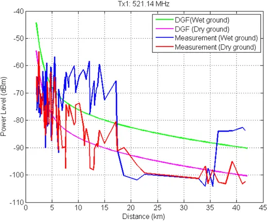
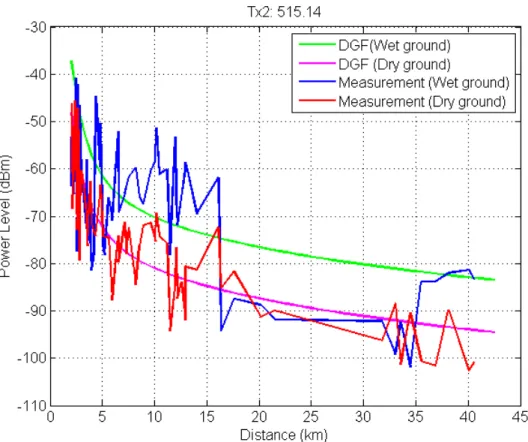
Measurement campaigns were carried out in Belém-PA city (1º27'18.62"S, 48°30'08.49"W), located in the Brazilian Amazon region. Power and electric field data from two DTV stations were collected. The nominal frequency of the transmitter Tx1 is 521.14 MHz and for Tx2 is 515.14 MHz. Additional information can be seen in Table II.
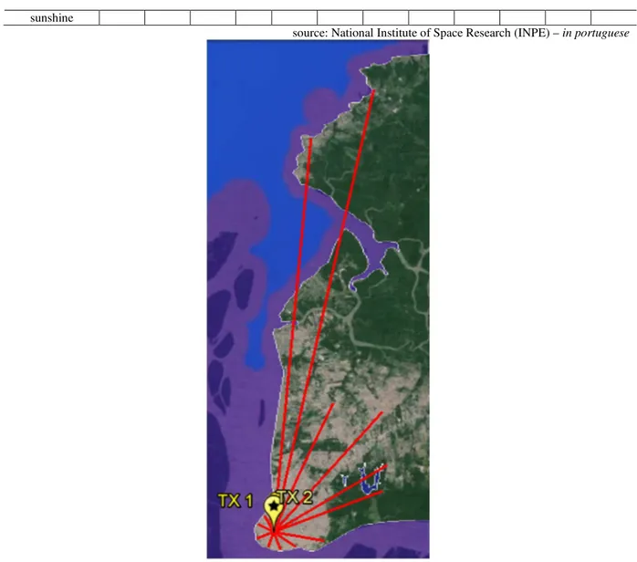
Measurements took place at 64 points spread across 14 radials. The selected points are spread over an area at a minimum distance of 2km and maximum distance of 43km from the Tx1. Due to the geometrical shape of the city, some radials have more points than others; the shorter radials have just two points. The information of the received power for all the radials was set out by taking the average power of the points located inside the concentric circles that were centered at each of the two transmitters Fig.3 shows a schematic map of the city.
There were two measurement campaigns during the year 2013 and these were designed to acquire power data in two Amazonian seasons: the rainy season and the dry season. The first measurement campaign was carried out during the months of March and April, a period described as the ‘Amazon winter’ with heavy and long-lasting rainfall. The second was in September during the Amazon summer when there were long periods of drought. Table III displays some climatological data about Belém.
The measurement setup involved installing an antenna dipole Anritsu MPP651A for the frequency range 470MHz to 1700MHz on the roof of a vehicle, with the aid of an aluminum tripod. A 3m long cable connected the antenna to the portable spectrum analyzer Site Master S332E (also an Anritsu) inside the vehicle, (Fig. 4). At each measuring point the receiving antenna Rx was redirected by taking the azimuth of Tx1 and Tx2 to obtain the maximum electric field strength.
TABLE II.INFORMATION ABOUT THE TRANSMITTING ANTENNAS
Transmitter Location Height (m) Range (MHz) Power Operation (kW)
Effective Radiated Power (ERP) (kW)
TX1 01º27’43”S/48º29’28”W 114.58 518-524 6.00 52.15
TX2 01º27’12”S/ 48º29’22”W 125.30 512-518 10.00 61.79
TABLE III.CLIMATOLOGICAL DATA OF BELÉM
Month Jan Feb Mar Apr May Jun Jul Aug. Sept Oct Nov Dec Precipitation
sunshine
source: National Institute of Space Research (INPE) – in portuguese
Fig. 3. Schematic map of Belém – Radial (red lines); transmitters (yellow); freshwater (blue region).
.
Fig. 4. Tripod and antenna installed on the roof of the vehicle used in the measurement campaigns
V. RESULTS
Brazilian Microwave and Optoelectronics Society-SBMO received 26 May 2014; for review 27 May 2014; accepted 23 Apr 2015
results of the proposed model and the measured data. The RMS errors and average differences of the curves are shown in Table IV. The higher power levels are observed for both the measured data and model output in the case of wet soil. In this case, the RMS error relative to Tx1 was 5 dB and 3.3 dB for Tx2. The RMS error for the dry soil is about 2 dB. In both cases, the error may be acceptable, despite the large variability of the measured data where the standard deviation is of the order of 13 dB.
The comparison of the mean difference of the curves provided another important result that could be used for validating the model (Fig.7 and Fig.8). It was observed that the DGF model had a mean difference between the curves of about 10.5 dB, which is a value close to the mean difference of the logarithmic trendline of the data (12.6 dB for Tx1 and 11.8 dB to Tx2). This average difference between the curves shows the ability of DGF model to distinguish the two climatic conditions under consideration. This factor is an innovative feature for using a deterministic propagation model in the UHF band.
Fig. 6. Comparison between the measured data and the DGF for the two seasons in the year (wet soil and dry soil) for the Tx2.
Brazilian Microwave and Optoelectronics Society-SBMO received 26 May 2014; for review 27 May 2014; accepted 23 Apr 2015 Fig. 8. Comparison between the DGF model and logarithmic trendline of measured data for the two seasons in the year
(wet soil and dry soil) for the Tx2.
TABLE IV.COMPARISON OF ERRORS AND AVERAGE DIFFERENCES IN THE DATA
Errors and Differences Tx1 Tx2
RMS (wet ground) (dB) 4.97 3.31
RMS (dry ground) (dB) 2.13 2.53
Mean difference of the logarithmic trendline of measured data (dB) 12.58 10.87
Mean difference of DGF model (dB) 10.18 11.80
VI. CONCLUSION
This paper proposed a propagation model for UHF band based on DGF that considers the climatic conditions of the environment, and that leads to deterministic radio propagation models.
DGF solutions were obtained from its expansion in eigenfunctions to predict the electromagnetic field during two different seasons in the Amazon region. Electromagnetic fields have been computed in their integral form, within appropriate boundary conditions. The main advantages of this methodology are as follows: i) the accuracy of the expansion in eigenfunctions (guaranteed by the spectral theory); ii) greater flexibility with regard to the characteristics of the medium; iii) the possibility of including sources with an arbitrary distribution current; iv) its application to isotropic and/or anisotropic media.
curves of the DGF model was 11 11 dB aprox; this this is relatively close to the value found with the logarithmic trendline of the measured data. The RMS errors were between 2-5 dB, which are values that are small enough to allow an effective application of this model.
The model investigated here enables an analysis to be conducted of the influence of climatic conditions on the transmission of electromagnetic signals in the UHF band, a factor that can lead to better planning of digital TV systems.
For future works, it is intended to apply the proposed model in different scenarios and frequency bands, and propose more precise values for the electric parameters of the Amazonian soil by solving the inverse problem.
ACKNOWLEDGMENT
The authors would like to thank the National Institute of Science and Technology-Wireless Communication (INCT-CSF) for its support.
REFERENCES
[1] C. Phillips, D. Sicker, and D. Grunwald, “Bounding the error of path loss models,” in Proc. IEEE Symp. New Frontiers Dynam. Spectrum Access Netw. (DySPAN), May 2011, pp. 71–82.
[2] P. Ding, C. W. Qiu, S. Zouhdi, S. P. Yeo, “Rigorous derivation and fast solution of spatial-domain Green’s functions for uniaxial anisotropic multilayers using modified fast Hankel transform method,” IEEE Trans Microw Theory Techn., vol. 60, no. 2, pp. 205-217, Feb. 2012.
[3] Y. P. Chen, L. Jiang, Z. G. Qian, W. C. Chew, “An augmented electric field integral equation for layered medium Green’s function,” IEEE Trans Antennas Propag., vol. 59, no. 3, pp. 960-968, Mar. 2011.
[4] A. Fallahi, B. Oswald, “On the computation of electromagnetic dyadic Green’s function in spherically multilayered media,” in IEEE IEEE Trans Microw Theory Techn.,vol. 59, no. 6, pp. 1433-1440, Jun. 2011.
[5] C. T. Tai, Dyadic Green’s Functions in Electromagnetic Theory. Scranton: Intext Educational, 1971.
[6] G. P. S. Cavalcante, D. A. Rogers, A. J. Giarola, “Analysis of electromagnetic wave propagation in multilayered media using dyadic Green’s functions,” Radio Sci., vol. 17, no. 3, pp. 503-508, May-Jun, 1982.
[7] G. P. S. Cavalcante and A. J. Giarola, “Optimization of radio communication in media with three layers,” IEEE Trans Antennas Propag., vol. AP-31, pp. 141-145, Jan. 1983.
[8] D. Liao and K. Sarabandi, “Near-Earth wave propagation characteristics of electric dipole in presence of vegetation or snow layer,” IEEE Trans. Antennas Propag., vol. 53, no. 11, pp. 3747-3756, Nov. 2005.
[9] L. Li, et al. “Cylindrical vector eigenfuntion expansion of Green dyadics for multilayered anisotropic media and its application to four-layered forest,” IEEE Trans. Antennas Propag., vol. 52, no.2, pp. 466-477, Feb. 2004.
[10] L. Li, et al. “Wave mode and path characteristics in a four-layered anisotropic forest environment”, in IEEE Trans. Antennas Propag., vol. 52, no. 9, pp. 2445-2455, Sept. 2004.
[11] T. Tamir, "On radio-wave propagation in forest environments," IEEE Trans. Antennas Propag., vol. AP-15, pp. 806-817, Nov. 1967. [12] D. K. N. Silva, A. W. Oliveira, W. J. S. Barros, J. P. L. de Araujo, G. P. S. Cavalcante, “Dyadic Green's functions for wireless system
to electric field prediction: A study case for digital TV systems in Amazon Region,” in Proc. Wireless Telecommunications Symposium - WTS 2014, Washington, D.C, Apr. 2014.
[13] G. P. S. Cavalcante, D. A. Rogers, and A. J. Giarola, "Radio loss in forests using a model with four layered media," Radio Sci., vol. 18, pp. 691-695, 1983.
[14] L. W. Li and P. N. Jiao, "Solution of the electromagnetic field in a forest model with four layered media," Chinese J. Radio Sci. (in Chinese) [or J. Guizhou Univ.-Natural Sci. (in English)], vol. 1(2) [or 6(3) and 7(1) (in two parts)], pp. 10-25 [or 24-31 and 41-52], 1986 (and 1989 and 1990, respectively).
[15] I. S Koh, Y. Lee, “Complete closed-form expression of dyadic Green’s function and its far- and near-field approximations for an impedance half-plane,” IEEE Trans. Antennas Propag., vol. 60, no. 8, pp.3794-3801, Aug. 2012.
[16] A. Y. Nikitin, F. J. Garcia-Vidal, L. Martin-Moreno, “Analytical expressions for the electromagnetic dyadic Green’s function in graphene and thin layers,” IEEE J. Sel. Topics Quantum Electron., vol. 19, no. 3, May/Jun. 2013.
[17] M. Zhou, S. B. Sørensen, E. Jørgensen, P. Meincke, O. S. Kim, O. Breinbjerg, “An accurate technique for calculation of radiation from printed reflectarrays,” IEEE Antennas Wireless Propag. Lett., vol. 10,pp. 1081-1084, 2011.
[18] M. N. M. Yasin, S. K. Khamas, “Measurements and analysis of a probe-fed circularly polarized loop antenna printed on a layered dielectric sphere,” IEEE Trans. Antennas Propag., vol. 60, no. 4, pp. 2096-2100, Apr. 2012.
[19] J. X. Yeo, Y. H. Lee, J. T. Ong, “Modified ITU-R slant path rain attenuation model for tropical region,” in Proc. Int. Conf. Information Communication and Signal Processing – ICICS, 2009.
[20] J. S. Mandeep, et al. “Modified ITU-R rain attenuation model for equatorial climate,” in Proc. 2011 IEEE Int. Conf. on Space Science and Communication, 12-13 July, 2011, Malaysia.
[21] Recommendation ITU-R P.618-10 Propagation data and prediction methods required for the design of Earth-space telecommunication systems. Genebra, 2009.
[22] ______ . ITU-R P.837-6 Characteristics of precipitation for propagation modelling. Genebra, 2012 [23] ______ . ITU-R P.839-3 Rain height model for prediction methods. Genebra, 2001.