Combinatorial Formulation of Ising Model Revisited
G.A.T.F. da Costa
∗and A. L. Maciel
†Departamento de Matem´atica
Universidade Federal de Santa Catarina
88040-900, Florian´opolis, SC, Brasil
Recebido em 15 de julho, 2002. Aceito em 12 de novembro, 2002.
In 1952, Kac and Ward developed a combinatorial formulation for the two-dimensional Ising model which is another method of obtaining Onsager’s famous formula for the free energy per site in the termodynamic limit of the model. Feynman gave an important contribution to this formulation conjecturing a crucial mathematical relation which completed Kac and Ward ideas. In this paper, the method of Kac, Ward and Feynman for the free field Ising model in two dimensions is reviewed in a self-contained way and Onsager’s formula is computed.
Em 1952, Kac e Ward desenvolveram uma formulac¸˜ao combinatorial do modelo de Ising em duas dimens˜oes que ´e um outro m´etodo para se obter a famosa f´ormula de Onsager para a energia livre por s´ıtio no limite termodinˆamico do modelo. Feynman fez importante contribuic¸˜ao a esta formulac¸˜ao conjecturando uma relac¸˜ao matem´atica crucial que completou as id´eias de Kac e Ward. Neste trabalho, o m´etodo de Kac, Ward e Feynman para o modelo de Ising em duas dimens˜oes sem campo ´e revisada e a f´ormula de Onsager ´e calculada.
I
Introduction
The aim of statistical physics is to understand the macro-scopic behaviour of a system formed by a very large number of particles from information about how they interact with each other. One way in which one can gain insight into this problem and thus about complex systems is by constructing idealized models which hopefully will exhibit some of the interesting features of real systems like phase transitions. Perhaps the most studied of these idealized models is the Ising model so called in honor to his first investigator, Ernst Ising (1900-1998).
The model was originally proposed as a simple model of ferromagnetism. In ref. [1] Ising investigated the model in one dimension and computed exactly its partition func-tion. In 1944, Onsager [2] considered the free field model in two dimensions and succeded to compute the partition function exactly. His method became known as the alge-braic formulation of the model. In 1952, Kac and Ward [3] developed a quite different method of obtaining Onsager re-sults known as the combinatorial formulation of the Ising model. Feynman developed the method farther and conjec-tured an identity relating functions defined on graphs and functions defined on paths on a square lattice [4, 7]. This identity is a crucial element in the combinatorial formulation of Kac, Ward and Feynman of the Ising model. The identity was later formally proved by Sherman [4-6], followed later
on by another proof by Burgoyne [7]. A somewhat simi-lar treatment to the combinatorial formulation of Kac, Ward and Feynman can be found in refs. [12-14]. An important variant of the combinatorial formulation using the so called Pffafians was developed by Green and Hurst [10].
The bibliography on the Ising model is vast and to give a full list of references is virtually impossible. A nice intro-duction to the model though is the paper by B. Cipra given in ref. [17]. Old surveys but still useful on the distinct formu-lations of the Ising model in two dimensions and its history can be found in refs. [10-11, 15-16] together with full lists of original references.
The objective of the present paper is to review in a self-contained way the calculation of the Onsager’s formula for the two dimensional free field Ising model in the combina-torial formulation of Kac, Ward and Feynman. Our presen-tation follows chapter V, section V.4, of Feynman’s book [9] and the paper by Burgoyne [7] although we have tried to be more careful with the mathematics involved than these ref-erences are.
The paper is organized as follows. In section II, the Ising model is defined. In section III and through its various sub-sections the combinatorial formulation of Kac, Ward and Feynman of the partition function is given. In section IV, Onsager’s formula for the free energy per site in the thermo-dynamic limit is computed.
∗e-mail: [email protected]
II
Definition of the model
The model is defined on a finite planar square lattice Λ
which mimic a regular arranjement of atoms in two dimen-sions. Suppose the lattice is embedded in the plane with sites having coordinates inZ×Z. To each siteiofΛit is assigned two possible states also called “spins” and denoted byσi, whereσi = +1orσi =−1. The interaction energy
between two particles located at thei-th andj-th sites and in the statesσiandσj, respectively, is postulated to be
Eij=
−Jσiσj ifi, jare n.n.
0 otherwise
(2.1)
where “n.n” stands for nearest neighbors, hence, in the Ising model it is assumed that the energy depends only on short range interactions. The energy is−J if the nearest neigh-bors are in the same state and+J if the states are distinct. The constantJwhich can be positive or negative is a param-eter for the model.
SupposeΛhasN2sites. Then, there are2N2
distinct con-figurations of the spins and, therefore,2N2
configurations
σ = (σ1, ..., σN2)of the system. CallS = {σ}the set of possible configurations of the system. The energy of each configurationσ∈Sis given by
Eσ=−J
n.n.∈σ
σiσj (2.2)
Suppose as well the system is at equilibrium temperature given byT. According to statistical mechanics, the proba-bilitypσto find the system in the configurationσis
pσ=
1
Z(β)e
−βEσ (2.3)
whereβ= kB1T,kBis Boltzmann constant, and
Z(β) =
σ
e−βEσ. (2.4)
is the so called partition function of the model. This simple looking function is simple to compute exactly only in one dimension, difficult but possible to compute exactly in di-mension two. In three didi-mensions nobody knows how to do it.
The exact knowledge ofZ(β)allows one to obtain infor-mation about the global behaviour of the system. Important quantities that are relevant to understand the physics of the system are all defined in terms oflnZor its derivatives. For instance, the free energy per lattice sitef in the thermody-namic limit is defined as
f =−kBT lim N→∞
logZ
N2 . (2.5)
A basic problem is to find a closed form, analytic expression forf. Phase transitions will appear as singularities inf or in one of its derivatives.
III
The combinatorial formulation
In the combinatorial formulation the partition function is ex-pressed as a sum over special subsets of the latticeΛcalled admissible graphs. Next, using a relation first conjectured by R. Feynman the resulting expression is converted into a product over paths. The final step towards the Onsager’s for-mula to be accomplished in section IV consists in deriving an integral representation for this product.
III.1 The partition function as a sum over
graphs
Let’s rewrite the partition function (2.4) as
ZN(K) =
σ1=±1
· · ·
σN=±1
n.n.
eKσiσj (3.1)
withK= + J
kBT. Noting thatσiσj =±1, it follows that eKσiσj =e±K= coshK±sinhK (3.2)
and
n.n.
eKσiσj = (1−u2)−x2
n.n.
(1 +σiσju). (3.3)
whereu= tanhKandx= 2N(N−1)is the number of bonds inΛ. Notice that|u|<1, for anyK.
Definition 3.1. An admissible graph is a connected or dis-connected subset ofΛwhose sites have even valence. Definition 3.2.Given an admissible graphG, define
IG(u) =
i∈G
u=uL (3.4)
where the product is over the bondsiofG.
Theorem 3.1. CallAthe set of all admissible graphsGof
Λ. Then,
ZN(u) = 2N
2
(1−u2)−N(N−1)
1 +
G∈A
IG(u)
(3.5)
Proof:To each pairi, jof nearest neighbors ofΛthere cor-respond a termuσiσjand a bond. Since the number of pairs
i, j of n.n. coincide with the numberx = 2N(N −1) of bonds ofΛthe product on the RHS of (3.3) is a polinomial of degreex, that is,
n.n.
(1 +uσiσj) = 1 + x
p=1
up n.n.
(σi1σi2)· · ·(σi2p−1σi2p)
(3.6)
The second summation is over all possible products of p
pairs(σiσj)of n.n. ofΛwhere a pair is not to occur twice in
the same product. To each pair(σiσj)there is associated a
bond connecting the neighborsiandjso to each product of
the second summation is over all graphs withpbonds. The graphs may have sites with valence1,2,3or4. The summa-tions over the spinsσi’s eliminate graphs having sites with
odd valence becauseσ
i = 0andσ3i = 0. The graphs
left are those whose sites have valence 2 or 4, thus admis-sible. If VG is the number of sites in a admissible graph
Gthen there is a factor2VG associated to it because each
site ofGcontributes a factor2coming from
σ2
i = 2and
σ4
i = 2. The sum overσincludes all theσiand not only
those with sitesiinG. The summation over the sites not in
Gwill give a factor2V−VGwhereV =N2is the number of
sites in the lattice, hence, in the end one gets the factor2V.
III.2 The partition function as a product over
paths
Let’s orient and number the bonds ofΛwith distinct pos-itive integersiand callΛwith this indexation a colored lat-tice.
Definition 3.3. A pathpoverΛis an ordered sequence of bonds each starting at the site where the previous one ended. The last bond ending at the site from which the first one started. Thus,pis closed. The path is subjected to the con-straint that it never goes backwards over the previous bond. A pathpis given by a word, that is, an ordered sequence of symbolsDiwhereidistiguishes the bonds ofΛ. A pathpis
then of the form
p=De1
j1D
e2
j2...D
el
jl (3.7)
for some l and where ei = +1(−1) if the path traverses
bondjifollowing the direction (opposite direction) assigned
to it. Because a path is closed it is defined to within its cir-cular order so that
De1
j1D
e2
j2...D
el
jl ≡D
e2
j2...D
el
jlD
e1
j1 ≡...≡D
el
jlD
e1
j1...D
el−1 jl−1
(3.8)
The inversionp−1ofpis given by
D−el
jl D
−el−1 jl−1 ...D
−e1
j1 (3.9)
We takepandp−1to be equivalent. Givenp, denote by[p]
the set of all paths equivalent top, that is, its circular permu-tations and their inversions.
Definition 3.4. A periodic path is one which has the word representation
(De1
j1...D
el
jl)
w (3.10)
for somel andw ≥ 2and where the subword in between brackets is nonperiodic.
Definition 3.5.A pathphas assigned to it a sign given by
s(p) = (−1)1+t (3.11)
wheretis the number of2π-angles turned by a tangent vec-tor while traversing p. A positive (negative) angle is as-signed to a counterclockwise (clockwise) rotation.
Example 1. See Figure 1a). A tangent vector starting at point eand traversing the path shown in Figure 1a) turns
once a total angle given by4.π2 = 2πafter its return toeso in this caset = 1ands(p) = +1. For the path in Figure 1b), the total angle turned is3π
2 −3
π
2 = 0sot = 0and
s(p) =−1.
r
e
✲ ❄
✻ ✛
(a)
r
e
✲ ❄
✻ ✛
✲
✛ ❄
(b)
Figure 1: Examples of paths with (a)s(p) = +1
and (b)s(p) =−1.
Remark.In section IV, instead of assigning an angle±π/2
to a turn we will count the contribution to the sign by assign-ingα=eiπ/4andα¯=e−iπ/4to each counterclockwise and
clockwise turn, respectively, and then in the end multiplying the result by−1. In the example above, one gets in this manner(eiπ/4)4=−1and(eiπ/4)3.(e−iπ/4)3= +1.
Mul-tiplying both results by−1, one recovers the correct sign for each path.
The sign of periodic paths.Suppose the sign of the nonpe-riodic path in between brackets in (3.10) is(−1)1+ts. Then,
the sign of the periodic path with periodwis (−1)1+wts.
Hence, the sign of a periodic path is−1 if its period is an even number and the sign equals the sign of the nonperiodic subpath if the periodwis an odd number.
Definition 3.6. To each pathpit is assigned the function
Ip(u)given by
Ip(u) =ul (3.12)
wherel=m1+...+mk, for somek, is the length ofp,mi
being the number of times bondiis covered byp, and the functionWp(u), “the amplitude ofp”, defined as follows:
Wp(u) =s(p)Ip(u) (3.13)
Theorem 3.2. The functionsIG(u)andWp(u),|u| < 1,
defined above satisfy the following relation:
1 +
G∈A
IG(u) =
[p]
[1 +Wp(u)] (3.14)
The product is over all inequivalent classes[p]of closed non-periodic paths. The summation is over all admissible graphs of the finiteN×Nplanar square latticeΛ.
Relation (3.14) is a simpler version suitable for the Ising model of a more general relation investigated by Sherman and Burgoyne in refs. [4-7]. The difference is that they assign to the bondsi of the lattice distinct parametersdi,
hence, in this case the functionsIGandWare given in terms
According to references [4,7,10,11], relation (3.14) first appeared as a conjecture in lecture notes by Feynman ( ref. [9], published only in 1972 and already mentioning ref. [4]). The first proof of it was achieved by Sherman in refs. [4,6] followed by another one later on by Burgoyne in ref. [7]. The simplest nontrivial case of the general relation is inves-tigated in ref. [8].
Below Burgoyne’s proof is essencially reproduced for the case|u|<1.
Proof:Expand the product over the distinct classes of non-periodic paths[p]as1(one) plus an infinite sum of terms of the form
Wp1(u)Wp2(u)...Wpk(u) =s
i
uri (3.15)
for some k wherep1, ..., pk is a set of nonperiodic paths
overΛ. The product on the r.h.s of (3.15) is over the bonds
i traversed by p1, p2, ...pk, and ri says how many times.
Ifp1, p2, ...pk traverse bondi, say,m1(i), ..., mk(i)times,
mj ≥0, respectively, thenri =ki=1mj(i). The signsis
the product of the signs ofp1, p2, ..., pk.
Let’s prove, first, that those terms having ri = 1, ∀i,
add up to
IG(u). Consider one of these terms with
as-sociated pathsp1, p2, ..., pk. Each bond in the set of bonds
traversed byp1, p2, ..., pk is traversed only once by one of
these paths. Thus, the only possible intersection if any be-tween any two of these paths in this case can occur only at a site of valence 4 and they cross each other like in Fig. (2.a) . Otherwise, they are disjoint. Thus, the set of bonds tra-versed by pathsp1, ..., pk constitute a graph whose vertices
have valence2 or4. This is an admissible graph. There-fore, to each term of the form of (3.15) with ri = 1, ∀i,
one can associate an admissible graph. This graph can be disconnected. This happen if the set of paths can be split into subsets completely disjoint which generate admissible graphs without any bonds and vertices in common.
Now, given an admissible graphGone can in general associate more than one term of the form of (3.15) with
ri = 1, each associated with a distinct set of paths. Let’s
see how this follows. The sites of an admissible graph have valence2 or 4. When a path strikes a site of valence 4 it has only3possible directions to follow. See Figures 2a, 2b, 2c. (The case in Fig. 2d is forbidden.) Then, any two terms associated to a given admissible graphGwill differ only in the types of crossings at the sites ofG. Since there are3
types of crossing per valence 4 site, the number of possible terms associated toGis3V whereV is the number of sites
ofGwith valence4.
A term has a sign which comes out from the contribu-tion of the signs of the paths associated to that term. Let’s see how the sign of a term comes out. A term witht1
cross-ings of type1(Fig. 2a.) has a sign which can be expressed as (−1)t1 wheret
1 includes selfcrossings of single paths
plus crossings between different paths. Indeed, since dis-tinct closed paths always intersect in a even number of cross-ings then(−1)t1will give the correct sign of the term which is the product of the signs of the individual paths. Let’s
asso-ciate to the crossings of typej= 2,3the sign(+1)t2(+1)t3 so that a term withtjcrossings of typej = 1,2,3has a sign
given by(−1)t1(+1)t2(+1)t3.
There areV!ways of distributingV =t1+t2+t3
cross-ings among the sites ofGbut since there aretjcrossings of
the typej,j = 1,2,3, one has to divideV!byt1!t2!t3!so
that the number of distinct terms withtjcrossings of typej
is
V!
t1!t2!t3!
(3.16)
These terms have the same factor I(G) = uL whereLis
the number of bonds ofG. Summing all these terms arising from a givenGand summing over all admissible graphsG
ofΛthe result is
G
{t}
V!
t1!t2!t3!(−1)
t1(+1)t2(+1)t3
I(G) (3.17)
where
t means summation over all t1, t2, t3 such that
t1+t2+t3=V. Using the multinomial theorem the
sum-mation over{t}gives(−1 + 1 + 1)V and one gets the result
GI(G).
If G is disconnected with l components Gi, i =
1,2, ..., l, each of them withtj,j = 1,2, ..., l, sites of
va-lence4andt
j=V, then applying the previous argument
to each component will giveI(G1)I(G2)...I(Gl) =I(G).
In view of the above result, the theorem could be equiv-alently stated by saying that the sum of terms withri > 1
for at least one of theiconverges to zero. Let’s prove this. LetGbe the set of all colored connected or disconnected subgraphsg of the colored lattice without valence 1 sites and such that ifgis connected thengis not a poligon, that is, a graph having valence 2 sites only. A disconnected graph is allowed to have some but not all of the components as poligons. The reason for excluding graphs which are poligons or having all components which are is that closed paths with repeated bonds over them are necessarily periodic and these are forbidden. The coloring ofgis that inherited from the colored lattice.
Giveng∈ G, calli1, ..., il(g)the bonds ofg. A termwg
associated togis of the form
wg=Wp1Wp2...Wpk= (sign wg)|wg| (3.18)
for somek and set of paths p1, ..., pk, which traverse the
bonds ofgonly, where
|wg|= l(g)
j=1
urij (3.19)
and rij is the number of times bond ij is traversed
by p1, ..., pk, that is, If p1, ..., pk traverse the i-th bond
m1(i), ..., mk(i)times,m≥0, respectively, then
rij =
k
a=1
Some but not all of them’s can be zero so thatrij ≥1with
at least onerij >1.
Let’s consider the set of all terms with the same effec-tive set of bonds{i}traversed, hence, the terms associated to a giveng. Within this set it’s possible in general to find terms with the same powers{r}and the same|wg|although
having distinct associated paths and possibly with different effective sign.
Let’s group together those terms which cover the same bonds ofgthe same number of times. Denote byWg,N(r)
the set of termswgwith the same powers{rij}and such that
l(g)
j=1rij =N, for fixedN. The summation over all terms
with repeated lines can now be expressed as
g∈G
{N}g
r(N)
wg∈Wg,N(r)
wg (3.21)
where
g∈G means summation over all elements in G;
{N}g means summation over all positive integersN
com-patible to the given graphg and such thatN ≥ l(g) + 1;
r(N) means summation over a set of positive integers
r1, ..., rl such that r1+...+rl = N and which are also
compatible tog; and, finally,
wg means summation over
all termswg∈ Wg,N(r).
Now the following remarks come to order. In the sec-ond summation, the caseN = l is excluded for it implies thatri= 1and in this case there can be no repeated bonds.
The caseN < lcorresponds to another elementg′∈ G. The
equality depends on the graphg. For instance, take the graph shown in Fig. 1b wherel+ 1 = 9. No nonperiodic closed path with repeated bonds can have lengthN = 9 because
l(g) = 8. The lengthNcan only be even and its minimum isN = 12. Hence, for this particular graphgthe summa-tion is over all even numbers greater or equal to 12. In any case, the set{N}ghas always infinite elements. Givengand
N ∈ {N}g, not all partitions ofN are allowed in the third
sum. For instance, given the graph in Fig. 1b andN = 12, the partition withrik = 1,∀k = 1, andri = 5can not be
associated to any allowed path. So, the set of integers{N} and partitions ofNmust be suitable to eachg.
Giveng, let’s consider now the partial sums
sn=
{N|N≤n}g
r(N)
wg∈Wg,N(r)
wg (3.22)
The goal is to show that in the limit n → ∞,sn goes to
zero. In ref. [7] its proved thatsn = 0. The argument of the
proof goes as follows.
Since the bonds ofg are covered the same number of times by all elements in the group, choose a bond ofg, say
b, which is traversed r > 1 times by all elements in the groupWg,N. This choice has to be done for each partition
r(N). Denote byPthe set of paths associated towg. Then,
P =P′
P′′whereP′is the set of those paths which
tra-verse bondbwhereasP′′is the set of those paths which do
not traverseb.
Given a pathp∈P′, letpcbe the path segment obtained
frompupon removal ofb. GivenP′={p, p′...}define
P′
c={pc, p′c, ...} (3.23)
This set has exactlyrpath segments. Collect under a same subgroupS the elementswg ∈ Wg,N having the property
that linebis covered exactlyrtimes by all elements in S
and they all have the same subsetP′
c withrpath segments
and the same subsetP′′. The setW
g,N is the union of such
subsets, that is,
wg∈Wg,N(r) wg=
S⊂Wg,N(r)
wg∈S
s(w)|wg| (3.24)
wheres(w)is the sign ofwg and|wg| = uN. Recall that
|u|<1so that|wg|<1.
The elements inside any givenScancel each other. De-note byq andethe elements ofS that are inP′ andP′′,
respectively. Suppose that the segmentsq1, ..., qrare all
dis-tinct. (For the case with repeated segments, see [7]). The terms inS are precisely those which can be obtained by joining the ends of the segments and this can be done in exactlyr!ways. This gives the possible termswgin the
sub-group. From the properties of the permutation group half of
N!permutations are odd and half are even and so the signs of half of the terms are positive and half are negative, hence, a cancellation takes place.
Using (3.14), the partition function of the two dimen-sional Ising model can now be expressed as a product over paths as follows:
ZN(u) = 2N
2
(1−u2)−N(N−1)
[p]
[1 +Wp(u)] (3.25)
The next step consists in expressing the product over[p]as an integral. This will be achieved in the next section.
IV
Paths amplitudes and Onsager’s
formula
Consider all paths that start at a fixed siteP1which we take
as the origin with coordinates(0,0)and end at the sitePn+1
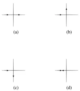
with coordinates (x, y)in n steps. Starting at (0,0) and whenever a site is reached there are four possible directions which a path can take (see Figure 2 and the Remark below). The patha)continues forward in the same direction of the previous step; b) it turns left 900 relative to the previous
step;c)it turns right900relative to the previous step;d)it
turns1800. To each one of this possibilities it is assigned
an “amplitude” which is given by: A)ufor the casea);B)
uαfor the caseb); C)uα¯ for the casec)andD)0 (zero) for the cased), where u = tghK and α = eiπ/4 is the
(a)
✲ ✲
(b)
✲ ✻
✲ ❄
(c)
✲✛
(d)
Figure 2: Directions which a path can take at a valence 4 site.
Remark.The lattice being finite it has a border so that when a path strikes a site on the border it may have there only two or three possible directions to follow. In the spirit of refs. [7,9] we shall neglect the border and derive the relevant for-mulas as if there was no border at all with the justification that in the limitN → ∞ which we shall take in the end of the calculation border effects dissapear. Of course, an-other approach would be to do everything on a toroidal lat-tice. In this case, however, relation (3.14) must be replaced by another more involved identity apropriate for the toroidal lattice ( given in refs. [4, 10] ). We shall restrict the presen-tation to the planar case only.
CallUn(x, y)the amplitude of arrival at(x, y)moving
upward in then-th step,Dn(x, y)the amplitude of arrival at
(x, y)moving downwards in then-th step,Ln(x, y)the
am-plitude of arrival at(x, y)moving from the left in then-th step, andRn(x, y)the amplitude of arrival at(x, y)moving
from right in then-th step.
If the path arrives at(x, y)moving upward in the n-th step then
Un(x, y) =uUn−1(x, y−1) + 0Dn−1(x, y−1)
+uαLn−1(x, y−1) +uαR¯ n−1(x, y−1) (4.1)
whereUn−1,Dn−1,Ln−1andRn−1are the amplitudes
as-sociated to the four possibilities to reach site(x, y−1). Re-lation (4.1) can be understood as follows. If(x, y−1) is reached going up a bond in the(n−1)-th step, there the amplitude isUn−1(x, y−1)so in then-th step as the path
follows the same direction of the previous step, by the rules
a)andA)above, a factoruis multiplied to the amplitude
Un−1(x, y−1). See Figure 3.
✻
(x,y)
r
r
✻
(x,y-1)
Figure 3:pgoes up to(x, y−1)and(x, y)
in the(n−1)-th andn-th steps.
If the site(x, y−1)is reached from the left in the(n−1) -th step (Figure 4), -the pa-th has to make a counterclockwise rotation to go to(x, y)in then-th step. By the rulesb)and
B)a factoruαshould then be multiplied to the amplitude
Ln−1(x, y−1).
✻ ✲
(x,y)
r
r(x,y-1)
Figure 4.pturns counterclockwise at(x, y−1)
to go to(x, y)in the n-th step.
The case that the path goes down to(x, y−1)in the(n−1) -th step and goes up to(x, y)in then-th step corresponds to a1800rotation. By rulesd)andD)the amplitude should be0.Dn−1(x, y−1). If the site(x, y−1)is reached from
the right the path has to make a clockwise rotation to go to
(x, y)(Figure 5). By the rulesc)andC)a factoruα¯should then be multiplied to the amplitudeRn−1(x, y−1).
✻ ✛
(x,y)
r
r
(x,y-1)
Figure 5.pturns clockwise at(x, y−1)to go to(x, y)in the n-th step.
Analogously, if a path arrives at(x, y)in then-th step going down the amplitude is given by the relation
Dn(x, y) = 0Un−1(x, y+ 1) +uDn−1(x, y+ 1)
If it arrives at(x, y)coming from the left then the amplitude is given by
Ln(x, y) =uαU¯ n−1(x−1, y) +uαDn−1(x−1, y) +uLn−1(x−1, y) + 0Rn−1(x−1, y) (4.3)
At last, if it arrives at(x, y)coming from the right the am-plitude is
Rn(x, y) =uαUn−1(x+ 1, y) +uαD¯ n−1(x+ 1, y)
+0Ln−1(x+ 1, y) +uRn−1(x+ 1, y) (4.4)
Of course to compute an amplitude using the above recur-sion relations it is needed the amplitude in the zero-th step. We shall follow the convention of reference [10], namely, that in the zero-th step a path arrives at the origin moving up-ward so thatU0(x, y) =δx,0δy,0andD0=R0=L0 = 0.
The amplitude to arrive in zero steps is one if the path ar-rives going upward at the origin and zero for any other point or any other direction of arrival.
Example 2. See Figure 6. Let’s compute the amplitude of arrival at site (2,1) in 3 steps moving upward in the third step. Only one path is possible in this case. Using the recur-sion (4.1),
U3(2,1) =uU2(2,0) + 0D2(2,0)
+uαL2(2,0) +uαR¯ 2(2,0) (4.5)
r
(2,1)
r
r r
(0,0) (1,0) (2,0)
Figure 6: The path in Ex. 2.
In the second step, the path moves to site (2,0) coming from the left soU2=D2=R2= 0andU3(2,1) =uαL2(2,0).
From (4.3),
L2(2,0) =uαU¯ 1(1,0)
+uαD1(1,0) +uL1(1,0) + 0R1(1,0) (4.6)
withU1 =D1 = R1 = 0so thatU3(2,1) = u2αL1(1,0)
where
L1(1,0) =uαU¯ 0(0,0) +uαD0(0,0)
+uL0(0,0) + 0R0(0,0) =uα¯ (4.7)
implying thatU3(2,1) =u3.
Example 3. Let’s now compute the amplitude of arrival at (2,1) in 3 steps moving from the left in the third step. In this case, the possible paths are shown in Figure 7a) and 7b).
r r
r r
✻ ✲
✲
(0,0) (1,0)
(1,1) (2,1)
(a)
r
✻
(0,0) (0,1)
r r r
(1,1) (2,1)
(b)
Figure 7: The paths in Ex. 3.
Using relation (4.3), the amplitude is
L3(2,1) =uαU¯ 2(1,1)
+uαD2(1,1) +uL2(1,1) + 0R2(1,1) (4.8)
Using (4.1),
U2(1,1) =uU1(1,0) + 0D1(1,0)
+uαL1(1,0) +uαR¯ 1(1,0) (4.9)
Since U1 = D1 = R1 = 0, one finds that U2(1,1) =
uαL1(1,0) =uαuα¯ =u2. Using (4.3), withD1 =L1 =
R1= 0,
L2(1,1) =uαU¯ 1(0,1) +uαD1(0,1)
+uL1(0,1) + 0R1(0,1) =uαu¯ (4.10)
Therefore,L3(2,1) = 2u3α¯.
Definition 4.1. The partial amplitude of a pathpof length
nis given by
Wp(u) =
αα u¯ n (4.11)
Definition 4.2 . The amplitude
pWp(n,P1)(u)of arrival atPn+1(x, y)from any direction innsteps is given by
Un(x, y) +Dn(x, y) +Ln(x, y) +Rn(x, y) (4.12)
Example 4. The partial amplitudes for the paths in Figure 6, 7a) and 7b) areu3,αu¯ 3andαu¯ 3, respectively. The
ampli-tude of arrival at (2,1) from any direction in 3 steps is, then,
u3+ 2 ¯αu3.
Definition 4.3. Fixnand callCn(x, y)the set of all paths
of lengthn starting at(0,0) and arriving at(x, y). Given
p∈CnandFn∈ B(x, y)where
B(x, y) ={Un(x, y), Dn(x, y), Ln(x, y), Rn(x, y)}
(4.13)
Define the extension ofFn(x, y), denoted by the same
sym-bol, so as to include sites (x, y) which can be reached only by a number m > n of steps but in this case set
Fn(x, y) = 0.
Lemma. The transform ofFn, the functionFn(ǫ, η),0 ≤
ǫ≤2πand0≤η≤2π, given by
Fn(ε, η) =
∞
x=−∞ ∞
y=−∞
is well defined and
Fn(x, y) = 2π
0
2π
0
eiεxeiηyFn(ε, η)dεdη
(2π)2 (4.15)
Proof: Fn(x, y) = 0for| x|> nor/and| y |> n. Then,
for fixednthe sums in (4.14) have only a finite number of terms.
Using (4.14), the transform ofUn(x, y)is:
Un(ε, η) =
∞
x=−∞ ∞
y=−∞
Un(x, y)e−iεxe−iηy (4.16)
Upon substitution of (4.1), and making the changey¯=y−1
it follows that
Un(ε, η) =ue−iηUn−1(ε, η)
+0 ¯Dn−1(ε, η) +uαe−iηLn−1(ε, η) +uαe¯ −iηRn−1(ε, η) (4.17)
Similarly, we obtainDn(ε, η),Ln(ε, η)andRn(ε, η):
Dn(ε, η) = 0Un−1(ε, η) +ueiηDn−1(ε, η) +uαe¯ iηLn−1(ε, η) +uαeiηRn−1(ε, η) (4.18)
Ln(ε, η) =uαe¯ −iεUn−1(ε, η) +uαe−iεDn−1(ε, η) +ue−iεL
n−1(ε, η) + 0Rn−1(ε, η) (4.19)
Rn(ε, η) =uαeiεUn−1(ε, η) +uαe¯ iεDn−1(ε, η) +0Ln−1(ε, η) +ueiεRn−1(ε, η) (4.20)
Callψn(ǫ, η)the matrix
ψn = Un Dn Ln Rn (4.21)
Then, from (4.17-20) we obtain that
ψn(ε, η) =ψn−1(ε, η)uM, (4.22)
where
M =
v 0 α h α h
0 v¯ α¯h αh¯
αv αv ¯h 0 ¯
α v α ¯v 0 h
(4.23)
withv=e−iη,h=e−iε,h=eiε,v=eiη andα=eiπ
4. Call1,2,3 and4 the directions shown in the Figure 8 below:
✻
1
2
✲ ✛
4
❄
3
Figura 8. Directions associated toMij.
Notice that the subindicesi, jofMijare in one-to-one with
the directions. Indeed,uM1j corresponds to the amplitude
of arrival at(x, y)( in(ǫ, η)space) coming up in the(n−1) -th step,∀j, but going up ifj = 1, down ifj = 2, coming from the left ifj = 3and coming from the right ifj = 4
in then-th step. Therefore,uM1jis the amplitude of arrival
at(x, y)( in(ǫ, η)space ) following directions1andj in the(n−1)-th andn-th steps, respectively. More generally,
uMij is the amplitude of arrival at(x, y)following
direc-tionsiandjin the(n−1)-th andn-th steps, respectively. From now on only closed paths starting at (0,0) and arriving at (0,0) innsteps will be considered. From (4.22) it follows that
ψn(ε, η) =ψn−1(ε, η)(uM)
=ψn−2(ε, η)(uM)2=· · ·=ψ0(uM)n (4.24)
Denote byψ0,i,1 ≤ i ≤ 4, the line matrix with the only
element distinct from zero and equal to 1 in the i-th col-umn. Letψ0 ≡ψ0,iaccording to whether the path arrives
at the origin moving up (i= 1), down (i= 2), from the left (i= 3) or from the right (i= 4), respectively. Then
Fn(ε, η) =ψ0,i(uM)nψ0T,i (4.25)
wherei= 1,2,3,4ifF =U, D, L, R, respectively, andΨT
is the transpose ofΨand
Fn∈Bn
Fn(ǫ, η) =
4
k=1
ψ0,k(ε, η)(uM)nψT0,k(ε, η) (4.26)
Given a4×4matrixA,ψ0,iAis the line matrix formed by
the elements in thei-th line ofA, that is,
ψ0,iA= Ai,1 Ai,2 Ai,3 Ai,4 (4.27)
soψ0,iAψ0T,i = Aii. Therefore, the sum overiequals the
trace ofA. Thus,
4
k=1
ψ0,k(uM)nψT0,k=T r(uM)n (4.28)
The total partial amplitude of arrival at(0,0)of closed paths moving in any direction innsteps given by (4.12) can be ex-pressed compactly as
Fn∈Bn
Fn(0,0) (4.29)
From (4.15), (4.26) and (4.28), it follows that
Fn∈Bn
Fn(0,0) = 2π
0
2π
0
T r(uM)ndεdη
(2π)2 (4.30)
To better understand relation (4.30), consider the matrix
unMn, for somen. An element(unMn)
⌋
(unMn)i1in+1=
4
i2,...,in=1
uMi1i2uMi2i3. . . uMin−1inuMinin+1. (4.31)
⌈ Recall thatuMi,jis the partial amplitude of a path arriving
at a site coming from directioniand going to the next site in one step following directionj. Thus, each term in the r.h.s. of (4.31) is the amplitude of a path of lengthnstarting atP1
coming from directioni1, going toP2following directioni2,
etc, and arriving at sitePn+1following directionin+1after
nsteps. The element(unMn)
i1in+1 gives the total partial amplitude of arrival atPn+1innsteps in(ǫ, η)space.
The terms in (unMn)
i1in+1 describe open as well as closed paths. Let’s see some examples.
Example 5. Take n = 5, i1 = 2 and i6 = 1. The
term M23M31M11M14M41 describes a path beginning at
P1 where it arrived coming from directioni1 = 2, going
toP2,P3, P4,P5 and to P6 following directionsi2 = 3,
i3= 1,i4 = 1,i5= 4andi6= 1, respectively. See Figure
9a).
Example 6. Take n = 6, i1 = i6 = 2 and the term
M23M31M11M14M42M22of(M6)22. This term describes
the closed path in Fig. 9b. The elements of Mn
out-side the diagonal have associated to them only open paths. This is implied by the simple fact that these elements have
i1=in+1. Closed paths are to be found only in the diagonal
elements since therei1 =in+1. However, open paths can
also be associated to some terms in the diagonal elements. Let’s see some examples.
r
P1 ✲ r P2
✻
r
✻
r P4
P3 ✛
r
P5 ✻
r
P6
(a)
r
r r
r r
r
P1
P6
P5
P2
P3
P4
✻ ❄
✲ ❄
✻ ✛
Figure 9: Paths in (a) Ex. 5 and in (b) Ex. 6. (b)
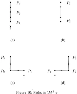
Example 7. Taken = 2, i1 = i3 = 1and the element (M2)
11=M11M11+M12M21+M13M31+M14M41with
u2(M2)11=u2v2+0+u2(αh)(αv)+u2(αh)(αv) (4.32)
To each one of the terms of(M2)
11 correspond the paths
(a), (b), (c) and (d), respectively, shown in Figure 10.
r
P3
r
P2
r
P1
(a)
✻
✻
✻
r
P1
r P2
(b)
✻ ❄
r
P3
P1
P2
r
r
✛ ✻
✻
(c)
✲ ✻
r
P1 P2
P3
r r
✻
(d)
Figure 10: Paths in(M2) 11
.
Example 8.Taken= 4and consider the following terms in
(M4) 11:
a)The termu4M
11M11M11M11=u4v4is the amplitude of
the open path shown in fig. 11 below.
r r r r r
✻
✻ ✻ ✻
Figure 11: Path(M11)4.
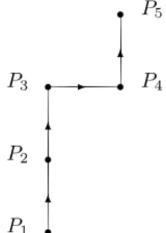
b) The term M11M11M13M31 = vv(αh)(αv) = v3¯hv
r r
r r
r
✻ ✻
✲ ✻
P1
P2
P3 P4
P5
Figure 12: PathM11M11M13M31.
c) The termu4M
13M32M24M41=u4(αh)(αv)(αh)(αv) =
u4α4(hh)(vv) = u4α4
is the amplitude of the closed path shown in Fig. 13:
r
r
P2
P1
P4
P3 r
r
✲ ❄
✻ ✛
Figure 13: PathM13M32M24M41.
In order to restrict to the elements ofMnhaving closed
paths we must take the trace ofMn. A closed path begins
at and return toP1afternsteps. Since it is closed it has to
covern/2horizontal bonds in one direction andn/2 hori-zontal bonds following the opposite direction. The same is true for the vertical bonds traversed byp. So, if the term
Mi1i2Mi2i3. . . Min−1inMinin+1 , in+1 = in, describes a
closed path, then the number ofh’s (v’s) equals the number of¯h’s (¯v’s) appearing in it. In this case, it’s possible to or-ganize the term into a product of pairsh¯h= 1andv¯v = 1
and the double integral inǫandη will give (2π)2 times a
product ofα’s andα¯’s. More precisely, the double integral over a closed path inT rMnequals
(2π)2αα (4.33)
where the first product is over all counterclockwise rotations and the second is over all clockwise rotations, so
αα= (−1)t(p) (4.34)
wheret(p) is the number of complete2πrevolutions per-formed by a tangent vector traversing the closed pathp. Re-mind that one has yet to multiply (4.34) by(−1)in order to get the complete signs(p)ofp.
If a path is open theh’s, ¯h’s (v’s,v¯’s) don’t match up into pairs. There will be left integrals of the form
2π
0
eikθdθ= 0, (4.35)
whereθstands forηorǫandk≥1, hence, the integrals inη
andεremove completely terms describing open paths. Let’s see examples.
Example 9. Taken = 1. In this case there are only open paths and
2π
0
2π
0
dηdεMij = 0, ∀i, j (4.36)
Example 10.Using (4.35), in ex. 7,
2π
0
2π
0
dηdε(M2)11= 0 (4.37)
Example 11.It is clear that
dεdη(Mn)ij= 0 ∀i, j (4.38)
ifn= 1,2,3, which is guaranteed by the fact that in a square lattice closed paths are possible only ifn ≥ 4. In the case
n= 2the path in Figure 10.b) is closed but it traverses the same edge back and its amplitude is thus zero.
Example 12. Using (4.35) in ex.8, for the term
M11M11M11M11=v4
2π
0
2π
0
v4dηdε= 2π
2π
0
e−4iηdη= 0. (4.39)
For the termM11M11M13M31=v3¯h,
2π
0
dηdεv3¯h= 0 (4.40)
For the term M13M32M24M41 = α4 which describes a
closed path the result
1 (2π)2
2π
0
dηdεα4=α4. (4.41)
follows which has the form (4.33-34) withα¯4≡1.
Given a closed path in (Mn)
ii, the inverse path is
present in some (Mn)
jj,j = i. For instance, in(M4)11
there are the closed paths shown in Fig. 14 given by the termsM14M42M23M31andM13M32M24M41.
r
P1
✲ ❄
✻ ✛
(a)
r
P1
✛
✻ ❄
✲
(b)
Figure 14: Paths (a)M14M42M23M31
In (M4)22 there are the terms M24M41M13M32 and
M23M31M14M42, with associated closed paths shown in
Fig. 15c and 15d, respectively:
r
P1 ✛
✻ ❄
✲
(c)
r
P1 ✲
❄
✻ ✛
(d)
Figura 15: Paths (c)M24M41M13M32
and (d)M23M31M14M42
In (M4)
33, there are the terms M32M24M41M13 and
M31M14M42M23 with associated closed paths shown in
Figure 16e) and 16f), respectively.
r
P1
✛
✻ ❄
✲
(e)
r
P1 ✲ ❄
✻ ✛
(f)
Figura 16. Paths (e)M32M24M41M13
and (f)M31M14M42M23
In (M4)
44, there are the terms M42M23M31M14 and
M41M13M32M24 with the associated closed paths shown
in Figure 17g) and 17h), respectively.
r
P1
✲ ❄
✻ ✛
(g)
r
P1 ✛
✻ ❄
✲
(h)
Figura 17. Paths (g)M42M23M31M14
and (h)M41M13M32M24
Note that (e) is the inversion of (a), (f) is the inversion of (c), (g) of (b), and (h) of (d).
So restricting to the diagonal terms of Mn which
amounts to take the trace of this matrix and then performing a double integration on the angles to eliminate open paths, dividing the result by 2 to eliminate inversions, and multi-plying the result by−ungives the total complete amplitude
( with the right signs ) to arrive back atP1innsteps
mov-ing in any direction. We have thus achieved the followmov-ing relation:
p(n,P1)
Wp(u) =−
1 2
1 (2π)2
2π
0
2π
0
dεdηT r(uM)n
(4.42)
The above result is restricted to a fixed siteP1. For the
fi-niteN×Nlattice withN2sites and disregarding boundary
effects, the total (independent of site) amplitude of closed paths of lengthnis:
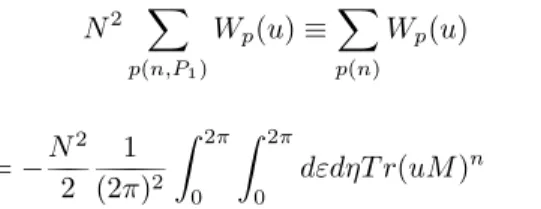
N2
p(n,P1)
Wp(u)≡
p(n)
Wp(u)
=−N
2
2 1 (2π)2
2π
0
2π
0
dεdηT r(uM)n (4.43)
Taking allN2 sites into account imply that given a closed
pathp(n), the summation
p(n)W(p)includes all circular
permutations ofp. To eliminate these the previous relation has to be divided byn. Then, the amplitude is given by
1
n
p(n)
Wp(u) =−
N2 2
1 (2π)2
2π
0
2π
0
dεdηT r(uM)
n
n
(4.44)
We notice that a nonperiodic path appearsn times in the sum but a periodic path of lengthnand periodwhasn/w
distinct starting points only and for this reason it appears
n/wtimes in the sum over paths. For instance, the periodic path(Dj1Dj2)(Dj1Dj2)(Dj1Dj2)of lengthn= 6and pe-riodw= 3has only two distinct starting points. The other equivalent periodic path isDj2(Dj1Dj2)(Dj1Dj2)Dj1. Af-ter division byn, periodic paths with periodwwill show up in the sum with a weight1/w. Thus, the above relation in-cludes all closed paths of lengthnover theN ×N lattice, periodic and nonperiodic, and excludes inversions and cir-cular permutations. The total amplitude of closed paths of any length is then given by the series
n
1
n
p(n)
Wp(u) =
∞
n=1
−N
2
2 1 (2π)2
2π
0
2π
0
dεdηT r(uM)
n
n (4.45)
whose convergence will be investigated below. We note that since the lattice is square, closed paths with nonzero am-plitude are possible only forn > 3but in view of relation (4.38) in Ex. 11 we can write the series in (4.45) starting fromn= 1.
With the above remarks,
∞
n=1 1
n
p(n)
[p]
[Wp(u)−
1
2(Wp(u)) 2+1
3(Wp(u))
3−...] (4.46)
In
[p] the first term is the sum ofWp(u)over all
nonpe-riodic paths. The other terms give the sum over all penonpe-riodic paths since any periodic path is the repetition of some non-periodic pathpwith period given byw= 2,3, .... In section 3.2 the sign of a periodic path was proved to be−1ifwis even and equal to the sign of its nonperiodic subpath ifwis odd. This explains the signs in the r.h.s of (4.46).
Since|u| < 1 then|W| < 1 and the series between brackets converges to ln(1 +W), and the r.h.s. of (4.46) equals to
p
ln(1 +Wp(u)) = ln
p
(1 +Wp(u)). (4.47)
a result to be used below.
Theorem 4.1.Take|u| ≤r < 14. Then, the series
∞
n=1
un(Mn) ij
n (4.48)
converges uniformily.
Proof: We have that|Mij| ≤ 1,∀i, j = 1,2,3,4, so from
(4.31) we get
|(Mn)ij |≤4n−1 (4.49)
and
un(Mn) ij
n
≤
4n−1|u|n
n (4.50)
The series
∞
n=1
(4|u|)n
n (4.51)
converges for|u| ≤ r < 1
4, hence, by WeierstrassM-test
the series (4.48) converges uniformly for|u| ≤r <1/4. We may conclude that the series ∞
n=1
−(uM)n
n
con-verges uniformly to the matrixln(1−uM)in the same in-terval.
We may now integrate the series term by term to get the series (4.45) which likewise converges uniformly in the same interval. Interchanging integration and summation in (4.45) yields
N2 2
1 (2π)2
2π
0
2π
0
dεdηT r
∞
n=1
−(uM)
n
n
= N 2
2 1 (2π)2
2π
0
2π
0
dεdηT rln(I−uM) (4.52)
From the previous analysis,|u| ≤r < 1/4. However, the r.h.s. of (4.52) is well defined in a bigger domain. Using the relation
T rln(I−uM) =lndet(I−uM) (4.53)
which is valid fordet(1−uM)= 0[18], we get
N2
2 1 (2π)2
2π
0
2π
0
dεdηlndet(I−uM) (4.54)
The determinant can be easily computed and one finds that
det(1−uM) = (u2+ 1)2−2u(1−u2)(cosε+ cosη) (4.55)
Taking the logarithm on both sides of relation (3.24) gives
lnZ(u)
N2 =ln2 + 2(1− 1
N)ln(coshK) +ln
p
[1 +Wp(u)]
(4.56)
or, using (4.45-47), (4.52,4.54),
lnZ(u)
N2 =ln2 + 2(1− 1
N)ln(coshK)
+ 1 8π2
2π
0
2π
0
dεdηlndet(1−uM) (4.57)
Using (4.55) withu=tanhKand the relations
u= 1
2sinh(2K)(1−u
2) (4.58)
(1 +u2)2=cosh2(2K)(1−u2)2 (4.59)
(1−u2) = 1
cosh22K (4.60)
gives
det(1−uM) =cosh−42K
(cosh2K)2
−(sinh2K)(cosη+cosε)] (4.61)
Onsager’s formula follows from (4.57) after taking the limitN → ∞:
− f
kBT
=ln2 + 1 2π2
π
0
π
0
dεdηln
(cosh2K)2
−sinh2K(cosη+cosε)] (4.62)
wheref is the free energy per site in the thermodynamical limit ( see (2.5)).
The integral in (4.62) can not be evaluated in terms of simple functions. The derivatives of the integral however can be expressed in terms of elliptic functions [2,15,19].
Set2k=tanh2K/cosh2K. Then,
−kf
BT
=ln2 +ln(cosh2K)
+ 1 2π2
π
0
π
0
dεdηln[1−2k(cosη+cosε)] (4.63)
Expanding the logarithm in powers ofkit follows that
−kf
BT
=ln2+ln(cosh2K)−
∞
n=1
(2n)! (n!)2
2
k2n (4.64)
The series converges for|2k(cosǫ+ cosη)| ≤4|k|<1. For
K=Kc( or temperatureTc= 2JkB−1ln−1(
√
2+1)) given by
2senh2Kc=cosh22Kc (4.65)
it diverges. ( Similarly, forJ <0which impliesk <0and divergence atTc= 2JkB−1ln−1(
√
2−1)). The internal energyUis given by
U =−kT2 ∂
∂T f
kT (4.66)
From (4.63),
U =−Jcoth(2K)
1 + (sinh22K−1)I(2K)
(4.67)
where
I(2K) = 1
π2
π
0
dǫdη
cosh2(2K)−sinh(2K)(cosǫ+cosη) (4.68)
By performing one of the integrals its found that
U =−Jcoth(2K)
1 + (2tanh22K−1)2
πF(k1)
(4.69)
wherek1 = 4kandF(k1)is the complete elliptic integral
of the first kind defined by
F(k1) =
π/2
0
(1−k2
1sen2θ)−
1
2dθ (4.70)
The elliptic functionF( see Ref. [19] ) has the property that
F→ln[4(1−k12)]−1/2 (4.71)
ask1→1−. So it diverges logarithmically atk1= 1, or at
the valueKcgiven by (4.65).
In relation (4.69) forU the functionF is multiplied by
(2tanh22K −1) which is zero at the critical point K
c.
Indeed, from the identity cosh2x = 1 +sinh2xrelation
(4.65) implies thatsinh(2Kc) = 1. Using this and (4.65),
tanh22Kc = 1/2follows. So the functionU is continuous
atKc.
The specific heat can be computed from the definition
C= ∂U
∂T (4.72)
It is given by
C=2k1
π (Kcoth2K)
2
{2F(k1)−2E(k1)
+2(tanh22K−1)G(k
1)} (4.73)
where
G(k1) =
π
2 + (2tanh 22K
−1)F(k1) (4.74)
andE(k1) is the complete elliptic integral of the second
kind, defined by
E(k1) =
π/2
0
(1−k21sen2θ)
1
2dθ (4.75)
which is well defined atk1= 1. From the exact result (4.73)
it follows that the specific heat is logarithmically divergent at the critical point.
References
[1] E. Ising, Zeitschrift f. Physik31, 253 (1925).
[2] L. Onsager, Phys. Rev.65, 117 (1944).
[3] M. Kac and J. C. Ward, Phys. Rev.88, 1332 (1952).
[4] S. Sherman, J. Math. Phys.1, 202 (1960).
[5] S. Sherman, Bull. Am. Math. Soc.68, 225 (1962).
[6] S. Sherman, J. Math. Phys.4, 1213 (1963).
[7] P. N. Burgoyne, J. Math. Phys.4, 1320 (1963).
[8] G. A. T. F. da Costa, J. Math. Phys.38, 1014 (1997).
[9] R. P. Feynman,Statistical Mechanics. A set of lectures.The Benjamin and Cummings Publishing Co., 1972.
[10] H. S. Green and C. A. Hurst,Order-Disorder Phenomena,
John Wyley and Sons.
[11] S. G. Brush, Rev. Mod. Phys.39, 883 (1967).
[12] N. V. Vdovichenko, Soviet Phys. JETP20, 477 (1965).
[13] Landau and Lifschitz,Statistical Physics, Addison-Wesley, 1969.
[14] M. L. Glasser, Am. J. Phys.38, 1033, 1970.
[15] C. J. Thompson,Mathematical Statistical Mechanics, Prin-centon University Press, 1972.
[16] G. F. Newell and E. W. Montroll, Rev. Mod. Phys.25, 353 (1953).
[17] B. A. Cipra, The American Mathematical Monthly,94, 937 (1987).
[18] F. Brauer and J. Nohel, The qualitative Theory of ODE, W. A. Benjamin, INC., 1969.