Adaptive method of lines for multi-component aerosol condensational growth and cloud droplet activation

(1)

GMDD

3, 1271–1315, 2010

Adaptive method of lines for CCN

activation

S. Arabas and H. Pawlowska

Title Page

Abstract Introduction

Conclusions References

Tables Figures

◭ ◮

Back Close

Full Screen / Esc

Printer-friendly Version

Interactive Discussion

Discussion

P

a

per

|

Dis

cussion

P

a

per

|

Discussion

P

a

per

|

Discussio

n

P

a

per

|

Geosci. Model Dev. Discuss., 3, 1271–1315, 2010 www.geosci-model-dev-discuss.net/3/1271/2010/ doi:10.5194/gmdd-3-1271-2010

Geoscientific Model Development Discussions

This discussion paper is/has been under review for the journal Geoscientific Model Development (GMD). Please refer to the corresponding final paper in GMD if available.

Adaptive method of lines for

multi-component aerosol condensational

growth and cloud droplet activation

S. Arabas and H. Pawlowska

Institute of Geophysics, University of Warsaw, Pasteura 7, 02-093 Warsaw, Poland

Received: 29 July 2010 – Accepted: 9 August 2010 – Published: 19 August 2010

Correspondence to: S. Arabas (sarabas@igf.fuw.edu.pl)

(2)

GMDD

3, 1271–1315, 2010

activation

Title Page

Tables Figures

◭ ◮

Back Close

Full Screen / Esc

Discussion

P

a

per

|

Dis

cussion

P

a

per

|

Discussion

P

a

per

|

Discussio

n

P

a

per

|

Abstract

The process of formation of cloud droplets on an ensemble of aerosol particles is mod-elled by numerous investigators using the method of lines (MOL). The method involves discretization of the aerosol size spectrum into bins whose position and width evolve with time. One of the drawbacks of the method is its poor representation of the aerosol 5

spectrum shape in the region between the unactivated aerosol mode and the activated cloud-droplet mode. An adaptive spectrum refinement procedure that improves the performance of the method is introduced and tested. A model of drop formation on multi-component aerosol is formulated for the purpose of the study. Model formula-tion includes explicit treatment of the drop temperature evoluformula-tion. Several examples of 10

the model set-up are used to demonstrate model capabilities. Model results are com-pared to those without adaptivity, and are comcom-pared to the Twomey’s formulæ. A C++ implementation of the model is available as an electronic supplement of the paper.

1 Introduction

Cloud droplets form on cloud condensation nuclei, CCN (Aitken, 1875, and the works 15

of his contemporaries). CCN are the atmospheric aerosol that contribute to the het-erogeneous nucleation of the water vapour. As a result, the microphysical properties of clouds (i.e. the size spectrum of cloud droplets) strongly depend on physicochem-ical properties of aerosol particles (see e.g., the review of McFiggans et al., 2006). Owing to the fact that the radiative properties of clouds and their ability to precipitate 20

are both dependant on characteristics of the size spectrum of cloud droplets (see e.g., the review of Stevens and Feingold, 2009), the description of the activation process is of importance to the studies on aerosol-cloud-climate interactions (e.g., Kulmala et al., 2009). This paper discusses a numerical method for studying the kinetics of aerosol growth by vapour condensation in the context of cloud-droplet activation. Presented 25

(3)

GMDD

3, 1271–1315, 2010

activation

Title Page

Tables Figures

◭ ◮

Back Close

Full Screen / Esc

Discussion

P

a

per

|

Dis

cussion

P

a

per

|

Discussion

P

a

per

|

Discussio

n

P

a

per

|

Aerosol growth by condensation of water vapour is conceptualized as a twofold dif-fusion process. First, there is the di_ffusion of water molecules towards the particle, and the condensation of water vapour on the drop surface. Concurrently, the latent-heat release triggers the diffusion of heat from the droplet, hence the system is akin to the wet-bulb thermometer described by Maxwell (1878). The chemical composition of the 5

growing particle and its curvature determine the vapour pressure over the droplet sur-face (K ¨ohler, 1936, and his earlier works), the driving factor of the diffusion process. Additional complexities are introduced when considering an ensemble of particles of different sizes (Howell, 1949; Kraus and Smith, 1949), with different shapes and sol-uble material content (Kornfeld, 1970), nuclei of different solubility (Fitzgerald, 1974), 10

and finally nuclei composed of di_fferent chemical species (Lee and Pruppacher, 1977) all competing simultaneously for the available water vapour. Yet another level of detail is reached when considering the feedback with the dynamics of the air (turbulence, entrainment and mixing), the interactions between the individual droplets (i.e. colli-sion/coalescence) or more sophisticated description of cloud chemistry, all being how-15

ever distant from the scope of this study. Numerical solutions of the problem had been repeatedly challenged using the fastest computers in the early years of electronic com-puting, starting with the studies of Mordy (1959) performed using the Swedish BESK computer, and the study of Neiburger and Chien (1960) carried out on the American SWAC.

20

The key complexity of the problem, from the mathematical standpoint, is the neces-sity to solve the partial differential equation describing the evolution of aerosol size spectrum. Analytical solutions to the problem (or semi-analytical estimates) can be derived only under significant approximations (see e.g., Squires, 1952; Twomey, 1959; Gelbard, 1990; Khvorostyanov and Curry, 2009, and references therein). Numerical 25

(4)

GMDD

3, 1271–1315, 2010

activation

Title Page

Tables Figures

◭ ◮

Back Close

Full Screen / Esc

Discussion

P

a

per

|

Dis

cussion

P

a

per

|

Discussion

P

a

per

|

Discussio

n

P

a

per

|

description of chemical properties of aerosol (see e.g., Chap. 5 in Williams and Loy-alka, 1991).

The partial differential equation may be reduced to a system of ordinary diff eren-tial equations (ODE) by spaeren-tial discretization of the inieren-tial size spectrum into sections with constant-in-time number of particles. The boundaries of these sections are then 5

allowed to evolve with time, hence the name moving-sectional technique/Lagrangian approach/full-moving structure (Jacobson, 1999, Sect. 14.5 therein) or method of char-acteristics (Gelbard, 1990), or method of lines (Debry et al., 2007). This approach was introduced by Howell (1949), and has since been used in modelling CCN acti-vation (e.g., Mordy, 1959; Neiburger and Chien, 1960; Fitzgerald, 1974; H ¨anel, 1987; 10

Feingold and Heymsfield, 1992; Nenes et al., 2001b; Grabowski et al., 2010). Such formulation of the model eliminates the computational difficulties inherent to numerical treatment of partial differential equations, and allows accurate description of the evo-lution of aerosol composition because particle properties such as mass of solute are retained throughout the computation.

15

The moving-sectional technique does pose computational difficulties because of the ODE system sti_ffness (see e.g., the discussion by Gelbard, 1990). The physical pro-cess of competition for the water vapour between the droplets of different sizes and chemical composition can be correctly resolved in a numerical solution only under suf-ficiently short time-steps. The approximations inherent to the bin-representation of the 20

aerosol size spectrum introduce significant uncertainties to the solution if low-resolution discretization is used (Korhonen et al., 2005). The issues of stiffness of the system and of appropriate time-step choice are addressed herein by using an adaptive Gear-type ODE solver. The issue of sensitivity of the results to the bin-number choice, being one of the factors causing discrepancies among results of different models (Kreidenweis 25

(5)

GMDD

3, 1271–1315, 2010

activation

Title Page

Tables Figures

◭ ◮

Back Close

Full Screen / Esc

Discussion

P

a

per

|

Dis

cussion

P

a

per

|

Discussion

P

a

per

|

Discussio

n

P

a

per

|

The following section of the paper covers model formulation and implementation. Sample results are discussed in the third section. First, a set of model runs without adaptivity is discussed revealing the sensibility of the results to parameters controlling the discretization of the initial aerosol size spectrum (Sects. 3.1 and 3.2). Second, the properties and e_fficacy of the adaptive size-spectrum discretization method are 5

presented (Sect. 3.3). Third, a comparison of the results with the predictions of the classic Twomey’s (1959) analytical formulæ is given (Sect. 3.4). The fourth section concludes the paper with a brief outlook on the possible applications of the discussed method within different domains of atmospheric research.

2 Model formulation and implementation 10

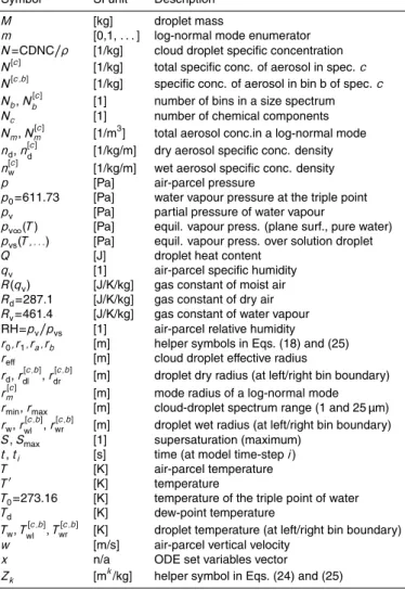
The model provides a description of the cloud-drop formation process at the initial stage of cloud-formation triggered by vertical air motion (i.e. in convective or orographic clouds). The model utilizes the method of lines (MOL) for numerically solving the so-called dynamic equation of aerosol growth by condensation. A list of symbols used in the text is given in Table 3.

15

2.1 Air-parcel system and its governing equations

The model describes an air parcel with the temperatureT, pressure p, and specific humidityqv being vertically displaced with constant velocity w. The parcel does not

exchange heat or mass with the environment and hence its heat budget (neglecting terms related to mass and heat content of droplets) is expressed as:

20

cp(qv)d T =

R(qv)T

p d p−lv(T)d qv (1)

where lv is the latent heat of evapouration, cp(qv)=cpvqv+cpd(1−qv) is the specific

heat capacity at constant pressure of moist air, andR(qv)=Rvqv+Rd(1−qv) is the gas

(6)

GMDD

3, 1271–1315, 2010

activation

Title Page

Tables Figures

◭ ◮

Back Close

Full Screen / Esc

Discussion

P

a

per

|

Dis

cussion

P

a

per

|

Discussion

P

a

per

|

Discussio

n

P

a

per

|

respectively;c_pvandcpddepict specific heat capacities at constant pressure for water

vapour and dry air, respectively.

The parcel’s pressure adapts instantaneously to the environmental value defined through the hydrostatic equilibrium. It follows that the pressure changes are driven by the vertical velocity of the parcel:

5

d p d t =−

pg R(qv)T

w (2)

wheregis the gravitational acceleration.

Physical characteristics of the aerosol suspended in the parcel are described by a set of probability density functions (PDFs) defining the size spectra of dry aerosol, each PDF corresponding to different chemical composition. The dry spectra n[_dc](rd) are

in-10

variant with time, are defined as a function of dry radiusrd, separately for each chemical

componentc. Each dry spectrum has a corresponding wet spectrumn[wc](rw,t) defined

analogously but varying with time. Bothn[_dc]andn[_wc] are expressed in terms of particle number per unit mass of moist air, and are referred to as specific concentrations. The model formulation is aimed at describing the growth of aerosol at high humidity, and 15

corresponding high relative water contents within particles of the wet spectra. The total mass of particles is assumed to be proportional to the third moment of the wet PDFs:

hr_w3_i=X c

1

N[c]

∞

Z

0

n[_wc](rw,t)rw3drw (3)

whereN[c]=R∞0 n [c]

w drw is the total specific concentration for a given chemical

compo-nent. For each wet spectrum a corresponding droplet temperature field T_w[c](r_w,t) is 20

also introduced.

(7)

GMDD

3, 1271–1315, 2010

activation

Title Page

Tables Figures

◭ ◮

Back Close

Full Screen / Esc

Discussion

P

a

per

|

Dis

cussion

P

a

per

|

Discussion

P

a

per

|

Discussio

n

P

a

per

|

with time-varying boundary conditions what results in the following form of the Fick’s first law and Fourier’s law (cf. e.g., Chap. 7 in Rogers and Yau, 1989):

d M d t

1

4πrw2

= D

rw

ρv−ρv|drop surface

(4)

d Q d t

1

4πrw2

= K

rw

(T−Tw) (5)

whereM=4πrw3ρl/3 is the mass of a drop of density ρl,ρv is the density of air in the

5

parcel,DandK are di_ffusion coe_fficients discussed below. The two di_ffusion equations are coupled via a heat budget equation:

d Q=Mcld Tw−lv(Tw)d M (6)

whereclis the specific heat capacity of liquid water.

Equations (4) and (5) evaluated with constant (or temperature-dependant) diffusion 10

coefficientsDandK represent the so-called continuum r ´egime in which the efficiency of diffusion is limited solely by the diffusivity of water vapour in air. Continuum r ´egime is applicable for particles of sizes larger than the free path of water molecules in air (i.e. rw≫0.1 µm). Evolution of size of much smaller droplets is described using the

molecular r ´egime, and the transition between the two r ´egimes may be approximately 15

allowed for by introducing a drop radius-dependency to the diffusion coefficient (Lang-muir, 1944, discussion of Eq. 52 therein). Here, we apply the transition r ´egime correc-tion factors of Fuchs and Sutugin (1970) in the form suggested for cloud modelling by Laaksonen et al. (2005):

D=D0

1+λD

r_w 1+1.71_·λD

rw +1.33· _λ

D

rw

2 (7)

(8)

GMDD

3, 1271–1315, 2010

activation

Title Page

Tables Figures

◭ ◮

Back Close

Full Screen / Esc

Discussion

P

a

per

|

Dis

cussion

P

a

per

|

Discussion

P

a

per

|

Discussio

n

P

a

per

|

K=K0

1+λK

r_w 1+1.71_·λK

r_w +1.33· _λ

K

r_w

2 (8)

whereD0is the diffusivity of water vapour in air,K0is the thermal conductivity of air,λD is the mean free path of water vapour in air, andλK is a length scale for heat transfer in air (the ratio of a mean free path to a characteristic length is called the Knudsen number). The two last are defined as:

5

λ_D=2D0(2RvTw)−1/2 (9)

λK= 4 5K0

T

p(2RdT)

−1/2

(10)

(Williams and Loyalka, 1991, Eqs. 6.6 and 6.33 therein).

The condensation/evapouration of water on/from the aerosol is the only source of changes in specific humidityqvand thus:

10

d qv

d t =−(1−qv)

4πρl

3

d d thr

3 wi

X

c

N[c] ₍₁₁₎

where the (1₋qv) term stems from the employment of specific quantities.

The density of water vapour at drop surface ρv|drop surface in Eq. (4) is assumed to

be equal to the equilibrium (saturation) value taking into account the Gibbs-Kelvin and Raoult e_ffects related to surface curvature and drop composition, respectively (the so-15

called K ¨ohler curve):

pvs=pv_∞(Tw)·a·exp

2σ RvTwρlrw

(12)

wherepv_∞is the equilibrium vapour pressure over plane surface of pure water,σis the

(9)

GMDD

3, 1271–1315, 2010

activation

Title Page

Tables Figures

◭ ◮

Back Close

Full Screen / Esc

Discussion

P

a

per

|

Dis

cussion

P

a

per

|

Discussion

P

a

per

|

Discussio

n

P

a

per

|

accordance with experimental data using the single-parameter representation of Pet-ters and Kreidenweis (2007, Eq. 6 therein):

a(r_w,r_d)= r

3 w−r

3 d

r_w3₋r_d3(1₋κ[c]₎ (13)

whereκ[c] is the single parameter representing chemical composition in spectrum c. The dry aerosol is assumed to be entirely soluble. A constant surface-tension coef-5

ficient σ=0.072 J/m2 is used (value for pure water at 298 K) in accordance with the parameterization of Petters and Kreidenweis (2007).

The specific heat capacities of dry aircpd, and water vapourcpvare assumed

con-stant (perfect gas), hence the latent heat of vapourisation is given by:

lv(T′)=lv0+(cpv−cl)·(T′−T0) (14)

10

and the equilibrium pressure over a plane surface of pure water (solution of the Clausius-Clapeyron equation) is given by:

pv_∞(T′)=p0·exp



 

lv0−(cpv−cl)·T0

R_v_·1

T₀−

1

T′ −1



 

_T′

T0

cpRv−_vcl

(15)

where T0, p0 and lv0 correspond to the triple-point values, and T′ denotes here the

temperature for which the formulæ are evaluated. The specific heat capacity of liquid 15

waterc_lis assumed constant.

2.2 MOL’s ODE system

(10)

GMDD

3, 1271–1315, 2010

activation

Title Page

Tables Figures

◭ ◮

Back Close

Full Screen / Esc

Discussion

P

a

per

|

Dis

cussion

P

a

per

|

Discussion

P

a

per

|

Discussio

n

P

a

per

|

PDFs with piecewise constant functions. Here, each bin (numbered byb) is defined by a constant-in-time number of particlesN[c,b] (per unit mass of air), and variable-in-time left and right boundariesr_wl[c,b](t) &rwr[c,b](t). The third moment of the particle size

spectrum is thus approximated using:

∞

Z

0

n[_wc]r_w3drw=

X

b

N[c,b]

r_wr[c,b] Z

r_wl[c,b]

rw3

r_wr[c,b]₋r_wl[c,b]

drw (16)

5

This allows expressing the time derivative of the total mass of wet aerosol without employing partial di_fferentials using:

d d thr

3 wi

X

c

N[c]=1 4

X

b X

c

N[c,b]· (17)

·

"

γr_wr[c,b],r_wl[c,b]dr

[c,b] wr

d t +γ

r_wl[c,b], r_wr[c,b]dr

[c,b] wl

d t





where 10

γ(r0,r1)=(3r₀4+r₁4−4r₀3r1)·(r0−r1)−2 (18)

An assumption thatr_wl[c,b]< rwr[c,b] is inherent in this formulation (cf. the discussion and

a related proof ofparticle ordering principlein Gelbard, 1990). The same discretization is applied to dry radiird, and particle temperatures Twintroducingr

[c,b] dl andr

[c,b] dr , and

T_wl[c,b](t) andT_wr[c,b](t), respectively. The MOL is thus applied to calculate the evolution of 15

rw(rd,t) andTw(rd,t) by discretizingrdand lettingtto be the only independent variable.

If the size spectra are discretized into adjacent bins then Twr[c,b]=T [c,b+1] wl , r

[c,b] dr =

r_dl[c,b+1] and r_wr[c,b]=r_wl[c,b+1]. Consequently, the state vector of the model assuming dis-cretization of the size-spectrum into N_b adjacent bins and N_c chemical components consists of:

(11)

GMDD

3, 1271–1315, 2010

activation

Title Page

Tables Figures

◭ ◮

Back Close

Full Screen / Esc

Discussion

P

a

per

|

Dis

cussion

P

a

per

|

Discussion

P

a

per

|

Discussio

n

P

a

per

|

– N_c_×N_bconstant concentrationsN[c,b]

– Nc×(Nb+1) constant dry radiir

[c,b] dl

– N_c×(N_b+1) variable wet radiir_wl[c,b]

– N_c×(N_b+1) variable temperaturesT_wl[c,b]

– variablep,T andqv

5

While still constant from the standpoint of the ODE solver,Nb,N [c,b]

andr_dl[c,b] change during the spectrum refinement, andNbbecomesN

[c]

(12)

GMDD

3, 1271–1315, 2010

activation

S. Arabas and H. Pawlowska Title Page Abstract Introduction Conclusions References Tables Figures ◭ ◮ ◭ ◮ Back Close

Full Screen / Esc

Printer-friendly Version Interactive Discussion Discussion P a per | Dis cussion P a per | Discussion P a per | Discussio n P a per |

The system of ODEs defines the derivatives of all the variables with respect to time as: d d t                            

r_wl[c,b]

T_wl[c,b]

qv p T                            

| {z } x =                               

D(λD,rw) ρ_lr_wl[c,b]

" pq_v R(q_v)T−

p_vsT_wl[c,b],r_wl[c,b],r_dl[c,b] R_vT_wl[c,b]

#

3

cl "

dr_wl[c,b] d t

l_v(T_wl[c,b])

r_wl[c,b] + T−T_wl[c,b]

r_wl[c,b]2

K(λK,rw) ρl

#

(qv−1)

πρ_l 3 P c P b

N[c,b]·

·

γhr_wr[c,b],r_wl[c,b]idr

[c,b] wr d t +γ

h

r_wl[c,b],r_wr[c,b]idr

[c,b] wl d t

−T Rpg(q_v)w

1

cp(qv) h_{T R}₍_q

v) p

d p d t−lv(T)

d q_v d t i                               

| {z }

F(x,t)

(19)

The drop-growth is described here using separate equations for drop-temperature and drop-radius evolution (see e.g., Vesala et al., 1997), as opposed to a single explicit 5

equation (the so-called Mason equation, Howell, 1949; Tsuji, 1950; Mason, 1957).

2.3 Initial conditions

The initial dry-aerosol size spectra and their chemical composition, initial temperature, pressure, humidity and the vertical velocity profile are the key parameters for each model run.

(13)

GMDD

3, 1271–1315, 2010

activation

S. Arabas and H. Pawlowska Title Page Abstract Introduction Conclusions References Tables Figures ◭ ◮ ◭ ◮ Back Close

Full Screen / Esc

Printer-friendly Version Interactive Discussion Discussion P a per | Dis cussion P a per | Discussion P a per | Discussio n P a per |

PDFs of tropospheric aerosol are generally well represented using a trimodal log-normal distribution (Whitby, 1978). The initial spectra of dry aerosol are thus defined for each model run using (Williams and Loyalka, 1991, Eq. 1.22 therein):

n[_dc](rd)=

1

ρ

X

m

N_m[c]

√

2πlnσ_m[c]

1 rd exp       −      ln rd rm[c]

√

2lnσ_m[c]

     2      (20)

whereN_m[c]is the total concentration in a mode,σ_m[c]is the geometric standard deviation 5

of a mode, andr_m[c]is the mode radius (all defined separately for each chemical compo-nent).N_m is generally reported as concentration (defined in terms of a unit volume, as opposed to unit mass as it is in case of specific concentrationnd) hence the division by

the air densityρin Eq. (20). The bins are initially equally spaced in logarithm of radius over the 1 nm–100 µm range what ensures accurate representation of the log-normal 10

shape of the initial spectra.

The initial spectra of wet aerosol are calculated by assuming an equilibrium state defined by:

T_wl[c] _t

=0=T [c] wr

_t

=0=T

dr_wl[c] d t

t=0

= dr [c] wr d t

t=0

=0

(21)

The initial values ofT,pandqvare chosen to describe the air properties slightly

be-15

(14)

GMDD

3, 1271–1315, 2010

activation

Title Page

Tables Figures

◭ ◮

Back Close

Full Screen / Esc

Discussion

P

a

per

|

Dis

cussion

P

a

per

|

Discussion

P

a

per

|

Discussio

n

P

a

per

|

2.4 Numerical solution

Integration of Eq. (19) without further approximations requires a numerical algorithm capable of solving a stiff ODE system (the stiffness of the system is confirmed e.g. by the significant ine_fficiency of the Adams-Moulton method with functional iteration). In addition, calculation of the initial wet spectra using an equilibrium condition defined 5

by Eqs (21) is not possible analytically. The latter problem is solved by employing an iterative root-bracketing procedure (using the Brent-Dekker method, cf. Sect. 2.6). The initial search interval for root-bracketing is defined using the dry radius for the lower bound, and the equilibrium value with the Gibbs-Kelvin effect neglected for the upper bound.

10

The ODE system is solved using the variable-order, variable-step backward diff eren-tiation formula (BDF) as implemented in the CVODE solver (Cohen and Hindmarsh, 1996, cf. Sect. 2.6 herein). In each time-step (numbered by i) the ODE system

dx/d t=F(x,t) defined by Eq. (19) is integrated by finding a root off(xi):

f(xi)= h X

k=1

αi ,kxi₋k+(ti−ti₋1)βiF(xi,ti)−xi (22) 15

using the Newton-Raphson iteration (herehvaries between 1 and 5, and defines the order of the method at the current time-step, andα_{i ,k} &β_i are variable coefficients). The iteration (with steps numbered byj) is of the following form:

x_ij+1=x_ij−f(xi)

f′₍_x_i₎=x

j i+

f(x_i) 1₋(ti−ti₋1)βi∂F∂x

(23)

The Jacobian matrix∂F/∂x is updated at least once every twentieth time-step. The 20

Jacobian is approximated by multiple evaluations of the right-hand side of Eq. (19) using the current, and slightly perturbed values ofx.

(15)

GMDD

3, 1271–1315, 2010

activation

Title Page

Tables Figures

◭ ◮

Back Close

Full Screen / Esc

Discussion

P

a

per

|

Dis

cussion

P

a

per

|

Discussion

P

a

per

|

Discussio

n

P

a

per

|

absolute tolerance was used in the calculations presented here). In addition, the solver is instructed to shorten the time-step if an unphysical condition is detected during eval-uation of the system right-hand side F(x,t) (e.g. if a positively-defined quantity has a negative value or if the left edge of a bin outruns its right edge).

The right-hand side of the ODE system is evaluated in the order presented in 5

Eq. (19). The integration is performed until a desired time (altitude) is passed, and an interpolated set of values for this time (altitude) is calculated and returned.

After each successful integration step, a spectrum-refinement procedure is carried out, if necessary, and in that case the integration over the last time-step is repeated. The conditions for triggering the spectrum-refinement are defined and discussed in the 10

following subsection. Each refinement causes a change of the length of x, which in turn results in reducing the current orderhto unity, and re-evaluation of the Jacobian matrix.

A solution of the problem in context of cloud-microphysical studies is a set of properties of the cloud-droplet spectrum such as cloud-droplet number concentration 15

(CDNC), liquid water content (LWC), average droplet radius (_hr_i), the standard devia-tion of the size spectrum (σr) and effective radius (reff). The k-th moment of the droplet

spectrum is evaluated, taking into account that the left-most (and right-most) bins may fall only partially in the assumed cloud-droplet region, using:

hrwki=Zk/Z0 (24)

20

where

Z_k=X c

X

b

N[c,b] r_wr[c,b]₋r_wl[c,b]

r_b₋r_a

r_wr[c,b]₋r_wl[c,b]

r_bk+1₋r_ak+1

k+1 (25)

wherer_a=max(rmin,r [c,b]

wl ),rb=min(rmax,r [c,b]

wr );rminwas set at 1 µm andrmaxat 25 µm.

Consequently:

– CDNC₌ρZ0

(16)

GMDD

3, 1271–1315, 2010

activation

Title Page

Tables Figures

◭ ◮

Back Close

Full Screen / Esc

Discussion

P

a

per

|

Dis

cussion

P

a

per

|

Discussion

P

a

per

|

Discussio

n

P

a

per

|

– LWC=4ρπρlZ3/3

– σr=

q

Z2/Z0−(Z1/Z0)2

– reff=Z3/Z2

2.5 The adaptive size-spectrum discretization scheme

The key task of the adaptive discretization scheme is to control the accuracy of the 5

discretization by splitting any overly wide bins into several smaller bins while the ODE system is integrated. Using the MOL nomenclature (Wouwer et al., 2001, Sect. 1.3 therein) it is thus anh-refinement of the spatial grid. Insertion of new bins takes place at discrete time levels only, namely when the ODE solver reaches its next internal time-step. Consequently, the grid adaptation procedure is decoupled from the ODE 10

integration and as such the static griding is employed. The method utilizes the so-calledfull restart as the ODE solver is reinitialised after each refinement event, and restarts with the lowest order. The restart and the reduction of the method order is a consequence of changing the length of the model state vectorx.

The criterion for triggering the division of a given bin is defined as follows. Bin splitting 15

happens whenever the ratio of the logarithm of the width of a given bin to its initial value reaches a certain limit. The limit was set at 2 for most of the simulations discussed in the text (save for the case of urban aerosol where 1.8 was used, cf. Sect. 3.3), mean-ing that no bin was allowed to double its width when viewed in logarithmic scale (the previous step of the solver is repeated each time new bins are added). Smaller limits 20

cause the algorithm to carry out the refinement earlier in time and hence increase the computational effort. Larger limits delay the refinement and at the same time increase the uncertainty inherent to the interpolation performed to calculate the drop tempera-tures and dry/wet radii at the edges of the newly created bins. No refinement takes place when the drop concentration in a given bin is below a certain level hereinafter 25

(17)

GMDD

3, 1271–1315, 2010

activation

Title Page

Tables Figures

◭ ◮

Back Close

Full Screen / Esc

Discussion

P

a

per

|

Dis

cussion

P

a

per

|

Discussion

P

a

per

|

Discussio

n

P

a

per

|

Any refinement event causes a full-restart of the ODE solver which, in turn, causes the solver to reduce the order, tighten its time-step, re-evaluate the Jacobian matrix, and consequently slow down the computations. For this reason, the number of bins into which a bin is split is chosen in a way ensuring no further splitting of any of the newly created bins will occur. The number of new bins added is thus chosen by dividingN[c,b]

5

by the tolerance. The new bins are spaced linearly in radius, and hence the specific concentration in each of the new bins is equal. The values of drop temperature and drop dry/wet radii at the newly introduced bin boundaries are linearly interpolated from the values at the boundaries of the bin being split.

The refinement criterion and the refinement procedure are local to a given bin and 10

thus different bins may be split at different times during the integration.

In principle, the presented approach replaces the single parameter of the discretiza-tion, the number of bins, with two new parameters: theinitial number of bins and the

tolerance. The former determines the uncertainty related to the discretization of the initial condition (initial dry radii). The later controls the uncertainty associated with the 15

final spectrum, and has a physical meaning, being the highest number of droplets al-lowed to reside in a bin laying in between the two modes of the final aerosol spectrum (i.e. modes of activated and non-activated particles).

2.6 Implementation of the model

The program is implemented in an object-oriented manner in C++. The implementa-20

tion is build upon the Boost.Units framework for dimensional analysis of the code at compilation time (Schabel and Watanabe, 2008) hence a physical unit is assigned to every variable/expression in the code with no performance penalty. The GNU Scien-tific Library (Galassi et al., 2009) is used for root-bracketing using the Brent-Dekker method (cf. Sect. 2.4 herein and Sect. 33.8 therein) and for root-polishing using the 25

(18)

GMDD

3, 1271–1315, 2010

activation

Title Page

Tables Figures

◭ ◮

Back Close

Full Screen / Esc

Discussion

P

a

per

|

Dis

cussion

P

a

per

|

Discussion

P

a

per

|

Discussio

n

P

a

per

|

Fortran-written VODE solver and a close relative of the Fortran-written LSODE solver. LSODE was used e.g. in Ghan et al. (1998), Nenes et al. (2001b) and Romakkaniemi et al. (2006) while two out of five models compared in Kreidenweis et al. (2003) and the model of Debry et al. (2007) were based on VODE.

The source code of the program is available as an electronic supplement of this pa-5

per and is released under the GNU General Public License. All model parameters are passed using UNIX-like command-line options. Toggling such settings of the model as transition r ´egime corrections, the Gibbs-Kelvin effect or the adaptivity do not require recompilation. Similarly, altering the numerical solution parameters such as the toler-ances or switching from BDF to Adams-Moulton method for ODE integration is possible 10

using command-line options. A web-based interface (written in HTML/PHP) allowing alteration of all model options, visualisation of single simulation results, as well as con-trol of parallel runs of simulations with different input parameters is included.

3 Example results

3.1 Example run without adaptivity: sea-salt/sulfate competition in marine 15

aerosol activation

Ghan et al. (1998) presented an analysis of relative importance of sea-salt and sulfate particles during CCN activation. The study was based on a series of simulations using a moving-sectional model of CCN activation. We use here a similar set-up for dis-cussing an example model run without adaptivity and relatively low spectral resolution 20

(45 bins over the 1 nm–100 µm radius range).

In the set-up the initial aerosol content of the air parcel is described by a sum of a single-mode log-normal distribution of ammonium sulfate aerosol, and a tri-modal log-normal distribution of sodium chloride aerosol. The parameters of all modes are listed in Table 1 and are based on measurement-data fits summarised in O’Dowd et al. 25

(19)

GMDD

3, 1271–1315, 2010

activation

Title Page

Tables Figures

◭ ◮

Back Close

Full Screen / Esc

Discussion

P

a

per

|

Dis

cussion

P

a

per

|

Discussion

P

a

per

|

Discussio

n

P

a

per

|

A steady updraftw=0.25 m/s is driving the changes in the parcel’s temperature, pres-sure, and relative humidity which are initially set at 280 K, 1000 hPa and 99%, respec-tively. The integration is performed for 250 s.

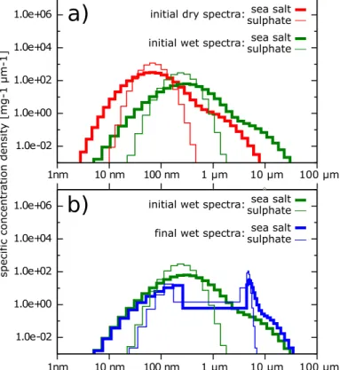
A summary of evolution of the aerosol spectra is presented in Fig. 1 (see figure caption for details). The shift towards larger sizes of the initial wet spectra (green 5

lines in Fig. 1a) with respect to the initial dry spectra (red lines) reflects the growth of particles up to RH=99% calculated assuming equilibrium condition (cf. O’Dowd et al., 1997, Fig. 4 therein). Further growth of the aerosol is calculated resolving the dif-fusion kinetics, and leads to activation of CCN and forming cloud-droplets (peaks on right-hand side of the final blue spectra in Fig. 1b). The final spectra of both sulphate 10

and sea-salt particles are distinctly bi-modal. The large-particle mode corresponds to cloud droplets, and is visible in both sulphate and sea-salt distribution. The small-particle mode corresponds to unactivated small-particles. The largest droplets were formed on sea-salt aerosol. For both aerosol components, the region of spectra between the two modes of the final PDFs is represented with a single bin spanning over an order 15

of magnitude in radius. This very section(s) is hereinafter referred to as the critical section(s) following Korhonen et al. (2005).

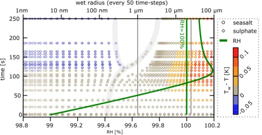
Figure 2 presents the time-evolution of particle sizes, particle temperatures (colour scale representing Tw−T), and the time/height profile of relative humidity. Wet radii

corresponding to the two chemical components considered are plotted using circles 20

and diamonds. The differences in wet radii for the same dry size (i.e. the differences arising from the differences in water activity for sea-salt and sulphate solutions) are most pronounced in the left-hand side of the plot (i.e. solution droplets of less than 10 nm in radius). Elsewhere, the two symbols (i.e. circles and diamond) overlap. The symbols are drawn every fiftieth time-step of the solver, and what follows the time-step 25

adjustments made by the solver may be observed.

(20)

GMDD

3, 1271–1315, 2010

activation

Title Page

Tables Figures

◭ ◮

Back Close

Full Screen / Esc

Discussion

P

a

per

|

Dis

cussion

P

a

per

|

Discussion

P

a

per

|

Discussio

n

P

a

per

|

supersaturation with respect to the plane surface of pure water. The second phase is characterised by a rapid growth of particles in the 0.5–5 µm range, and continuous increase of the relative humidity until reaching a maximum value of 100.2%. In the third phase, occurring roughly from 120 s until 150 s, the rate of growth of particles stabilizes throughout the whole spectrum, with the exception of the region separating 5

the unactivated and activated modes. There, one of the bin-boundaries undergoes a different evolution for sulphate and sea-salt aerosol, initially having equal volume of dry material (highlighted with the thick light-gray bifurcated line in the background in Fig. 2). The boundary of the very bin in the sulphate spectrum becomes the smallest one in the activated part of the spectrum, while the one of the sea-salt aerosol is the 10

largest one in the unactivated part of the spectrum. The relative humidity decreases during the third phase. Finally, the fourth phase of the growth represents a quasi-equilibrium state with activated droplets steadily growing at almost constant relative humidity.

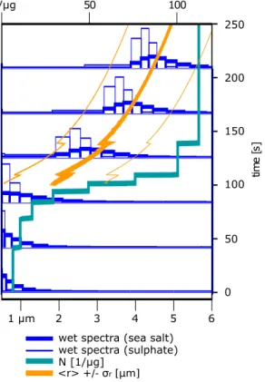
The characteristics of the cloud-droplet spectra (spectrum moments calculated over 15

the 1 µm–25 µm radius range) are presented in Fig. 3. The shapes of both spectra (sea-salt and sulphate solution droplets) are plotted at six intermediate altitudes (his-tograms constructed with thick and thin blue lines, respectively). The cloud droplet specific number concentration (turquoise line) increases till about 140 s (35 m), and stays constant afterwards. The mean radius (thick orange line) increases continuously 20

with height from the onset of drop formation till the end of the model run. The standard deviation of the drop radius (thin orange lines) stays approximately constant. The drops formed on sulphate aerosol dominate in the small-size part of the spectrum, while the sea-salt aerosol took part in formation of the largest drops.

3.2 Sensitivity to the discretization resolution (without adaptivity) 25

(21)

GMDD

3, 1271–1315, 2010

activation

Title Page

Tables Figures

◭ ◮

Back Close

Full Screen / Esc

Discussion

P

a

per

|

Dis

cussion

P

a

per

|

Discussion

P

a

per

|

Discussio

n

P

a

per

|

and the integration process. As pointed out in Kreidenweis et al. (2003) the droplet number concentrations obtained with models relying on the moving-sectional technique are sensitive to the number of bins used for the discretization of the aerosol spectra. To assess the degree to which the choice of the number of bins used to represent the initial spectrum influences the results, a set of simulations run with di_fferent number 5

of bins is compared. The variability of the results due to changes in discretization parameter is compared with the variability associated with the aerosol physical and chemical properties, and the vertical air velocity.

Four tri-modal aerosol distributions corresponding to properties of aerosol of different air-mass types are taken into account. Their parameters are listed in Table 2 and are 10

based on themarine,clean continental,average backgroundandurbancases reported in Whitby (1978). For each distribution, a nuclei mode, an accumulation mode, and a coarse mode is defined. The spectra are assumed to represent the sizes of dry particles. This is the set of cases used in Nenes et al. (2001b) for studying the influence of aerosol characteristics on cloud radiative properties using a moving-sectional model 15

of CCN activation.

For each of the considered initial aerosol size distributions the calculations are car-ried out separately assuming pure ammonium sulphate and pure sodium chloride aerosol, and for three different updraft speeds, namely 0.25, 1 and 4 m/s. Calcula-tions are performed until reaching 125 m. Each set-up (defined by one of the four size-20

spectra, one of the two chemical compositions, and one of the three vertical velocities) is tested with 54 different numbers of bins ranging from 30 to 300, with a step of 5. All other model parameters are defined as in the example run described in Sect. 3.1.

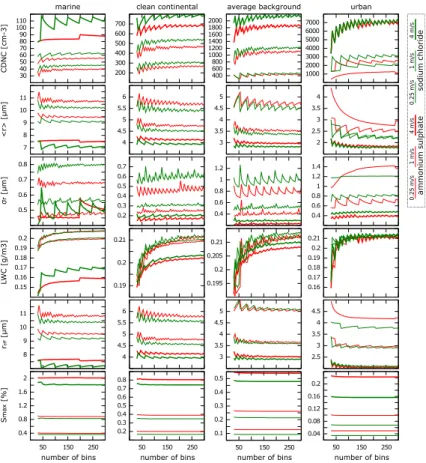
Figure 4 presents the results from all 1296 model runs. Six quantities are compared, out of which five represent the final values reached at the altitude of 125 m above the 25

initial level: the drop concentration CDNC, the mean radius of the droplets _hri, the standard deviation of the radiusσr, the effective radiusreffand the liquid water content

LWC. The sixth quantity is the maximum supersaturation Smax=max(RH−1)

(22)

GMDD

3, 1271–1315, 2010

activation

Title Page

Tables Figures

◭ ◮

Back Close

Full Screen / Esc

Discussion

P

a

per

|

Dis

cussion

P

a

per

|

Discussion

P

a

per

|

Discussio

n

P

a

per

|

are sensitive to the number of bins used to represent the initial spectra of aerosol. The maximum supersaturation is the only quantity not exhibiting significant variation. The variability associated with the changes in the number of bins is in some cases stronger that due to different chemical composition or updraft velocity (e.g. σr in the

marine case). Gradual increase of the number of bins does lead to the convergence 5

of the result to an asymptotic value; however, arguably 300 bins is not a sufficient number in some cases. Clearly, the results obtained with less than 100–150 bins are characterised by significant uncertainty.

The observed range of values of CDNC is roughly in line with observations reported in Kreidenweis et al. (2003) and Korhonen et al. (2005). While the differences in the 10

model formulations, and the di_fferences in model set-ups rule out direct comparison of the results, it is worth to mention several of observations from the two mentioned stud-ies. In both cases the focus was given to the drop number concentration. Kreidenweis et al. (2003, Par. 22 and Fig. 8 therein) compared results from four di_fferent models, running them with different number of bins ranging from 20 to 100. The bins were 15

spaced equally in logarithm of radius and in all cases covered at least two decades of the 1 nm–10 µm size range. The variability of drop number concentrations was ob-served for all of the models. The discrepancies between the results obtained with the same model but with different number of bins reached ca. 10%. Korhonen et al. (2005) compared results obtained using five different activation schemes run at low spectral 20

resolution (10 bins within the 10 nm–1.5 µm range) with a high-resolution run in which 500 bins were used. The variations were analysed separately for marine, rural, and urban aerosol, and for a variety of vertical velocities (all below 1 m/s). Predictions of the most accurate low-resolution models differed from the high-resolution calculations by roughly, up to 1%, 10% and 50% for marine, rural, and urban aerosol, respectively 25

(Korhonen et al., 2005, Fig. 3 therein).

(23)

GMDD

3, 1271–1315, 2010

activation

Title Page

Tables Figures

◭ ◮

Back Close

Full Screen / Esc

Discussion

P

a

per

|

Dis

cussion

P

a

per

|

Discussion

P

a

per

|

Discussio

n

P

a

per

|

critical section on the total number of activated cloud droplets, as well as broadening of the cloud droplet size spectrum with increasing number of bins used. Ghan et al. (1998) used bins of equal number of particles, as opposed to the present logarithmic layout, effectively increasing the discretization resolution near the critical section(s). 3.3 Example results with adaptivity

5

The same series of simulations as presented in the previous section was repeated with adaptivity. The tolerances were set to min(0.5%_·N_m, 50 µg−1) using N_m of the accu-mulation mode (see Table 2) giving 0.3 µg−1, 4 µg−1, 11.5 µg−1and 50 µg−1for marine, clean continental, average background and urban cases, respectively. The results of multiple simulations with adaptivity are summarized in Fig. 5 intended for direct compar-10

ison with Fig. 4. The previously observed variability of the results with varying number of bins is visibly suppressed confirming the efficacy of the proposed method. The qual-ity of the results (i.e. the stabilqual-ity with regard to the number of initial bins) obtained with low initial number of bins is significantly enhanced, in particular in the case of LWC. This suggests that introduction of the adaptivity helps the model to correctly resolve 15

both droplet mass- and droplet number-related quantities, even though the model is formulated using particle number distributions. Both the effective radiusreff and

cloud-droplet number concentration CDNC do not exhibit virtually any variability (both being the very focus quantities of the studies on cloud-radiative properties, cf. e.g., Brenguier et al., 2000, and references therein). Comparison of Figs. 4 and 5 confirms that i) the 20

sensitivity of the model-predicted values of CDNC to number of bins observed by Krei-denweis et al. (2003) and Korhonen et al. (2005) is related to the poor representation of the spectrum shape near the critical section(s); ii) the adaptive discretization scheme correctly identifies the critical section(s); iii) the proposed refinement strategy helps to limit the uncertainty of the results.

25

(24)

GMDD

3, 1271–1315, 2010

activation

Title Page

Tables Figures

◭ ◮

Back Close

Full Screen / Esc

Discussion

P

a

per

|

Dis

cussion

P

a

per

|

Discussion

P

a

per

|

Discussio

n

P

a

per

|

ca. 50 bins on the abscissa (i.e. roughly the number of bins needed to obtain conver-gence with adaptivity) is, in general, lower than the number of bins needed to obtain convergence without adaptivity. Consequently, the method offers a reduction of com-putational effort needed to obtain results of a given precision.

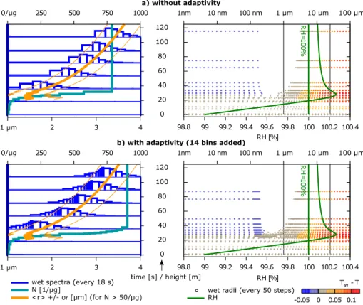
An in-detail comparison of one of the simulations presented in Figs. 4 and 5 is pre-5

sented in Fig. 7a (without adaptivity) and 7b (with adaptivity). The vertical velocity was set at 1 m/s, the aerosol size spectrum was initialized with the average background

distribution, and the composition was assumed to be pure ammonium sulphate. To en-hance the readability of the figure by lowering the number of bins, the initial number of bins was set at 55, and the tolerance was decreased to 46 µg−1. During the simulation 10

with adaptivity 14 bins were added to the spectrum. There are two most evident di_ff er-ences among the plots in Fig. 7a and b. First, the final concentration calculated with adaptivity is about 15% higher, and consequently the predicted average drop radius is smaller. Second, the shape of the spectra at di_fferent heights is asymmetric for the case without adaptivity.

15

Enabling adaptivity, and thus increasing the resolution of the discretization in the very region of the spectrum where the drop-growth is most vigorous, allows the model to re-solve the shape of the left-hand side slope of the droplet spectrum. This suggests that the asymmetry of the drop spectrum near cloud base, predicted by the model without adaptivity, is a numerical artifact. Finding support for this observation in experimental 20

data is difficult as most of the cloud droplet spectrometers nowadays are optical instru-ments which, for physical reasons, cannot sense the smallest (i.e.<1.5 µm in radius) cloud droplets (see e.g., Fig. 10a in Lawson and Blyth, 1998, presenting the cloud spectra 50 m above cloud base as measured by three different instruments).

The ability of the model to faithfully resolve the spectrum shape at the very onset of 25

(25)

GMDD

3, 1271–1315, 2010

activation

Title Page

Tables Figures

◭ ◮

Back Close

Full Screen / Esc

Discussion

P

a

per

|

Dis

cussion

P

a

per

|

Discussion

P

a

per

|

Discussio

n

P

a

per

|

Comparison of the right-hand side panels of Fig. 7a and b suggests that the adap-tivity contributes as well to a better representation of the transition-r ´egime corrections in the model. The increase of the number of bins near 100 nm results in probing the transition-r ´egime interpolation formulæ at denser intervals.

3.4 Comparison with the Twomey’s analytical formula 5

In his seminal paper of 1959, Twomey presented a derivation of an analytical solution of the CCN activation problem. His solution offers two robust expressions for upper bounds of maximum supersaturation and cloud drop concentration. The latter have since been widely used in cloud modelling (cf. e.g., the discussion of Grabowski et al., 2010, and references therein).

10

In the formulæ of Twomey (1959) the supersaturation is expressed in terms of the dew-point elevation:

E=Td(pv)−T (26)

where the dew-point temperatureTd=p− 1

vs(pv) is the inverse function of the equilibrium

vapour pressure, and pv=pv(p,qv) is the partial pressure of water vapour. In the

15

Twomey’s solution, the upper bound of the maximum dew-point elevation is a function of vertical air velocityw, and two parameters describing the aerosolkTandcT:

Emax<

"

1.63×10−3·w3/2 cT·kT·B(3/2,kT/2)

#_k1 T+2

(27)

where B denotes the Euler beta function, the 1.63_×10−3 coefficient corresponds to temperature of 10◦C and pressure of 800 hPa, the vertical velocityw is expressed in 20

centimetres per second,cT is expressed in cm− 3

and E is expressed in K. The upper bound of the drop concentration is expressed as a function ofkT,cT andEmax:

(26)

GMDD

3, 1271–1315, 2010

activation

Title Page

Tables Figures

◭ ◮

Back Close

Full Screen / Esc

Discussion

P

a

per

|

Dis

cussion

P

a

per

|

Discussion

P

a

per

|

Discussio

n

P

a

per

|

where CDNC is expressed in cm−3.

Twomey (1959) has given three sets of example value pairs forkT andcT, including

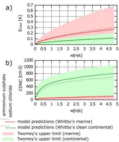
two formarineaerosol and one forremote continental aerosol. Twomey’s relations are compared here with results of multiple simulations using the present model. Aerosol spectra from (Whitby, 1978) are used for defining the dry aerosol spectra. The

ma-5

rineandclean continental distributions defined in Table 2 are compared with Twomey’s

marine (A) (kT=1/3,cT=125 cm− 3

) and remote continental (kT=2/5, cT=2000 cm− 3

) cases, respectively. The model was initialized at temperature of 10◦C, pressure of 800 hPa, and relative humidity of 99.5% to closely resemble Twomey’s set-up. The initial number of bins was set to 40, simulations were run with adaptivity, with the toler-10

ance set at 5 µg−1. As with previous set-ups, all calculations were done both for pure ammonium sulphate and pure sodium chloride for the purpose of comparing the de-gree to which the results are sensitive to chemical composition as opposed to other parameters. For both chemical species (i.e. NaCl and (NH4)2SO4) and both size

spec-tra (i.e. marine and continental) the model was run at 25 different updraft velocitiesw

15

between 0.01 and 5 m/s (with an increment of 0.2 m/s).

In Fig. 8 the model results are compared with the values obtained using the Twomey’s formulæfor the upper bounds of drop concentration and maximum dew-point elevation. The plotted values of drop concentration correspond to the concentrations at the alti-tude of 200 m above the initial altialti-tude thus in the fourth stage of the activation process 20

when the concentration is nearly constant. The maximum dew-point elevation corre-sponds to the difference between the dew-point and the parcel temperature at the time-step of the maximum relative humidity (supersaturation). The dew-point temperature is computed by iteratively (Steffensen method, cf. Sect 2.6) inverting Eq. (15).

The comparison clearly shows that the model predictions do fall below the upper-25

(27)

GMDD

3, 1271–1315, 2010

activation

Title Page

Tables Figures

◭ ◮

Back Close

Full Screen / Esc

Discussion

P

a

per

|

Dis

cussion

P

a

per

|

Discussion

P

a

per

|

Discussio

n

P

a

per

|

noteworthy; however, no further quantitative analysis seem feasible taking into account the degree of approximation employed in the Twomey’s solution (including neglect of the Gibbs-Kelvin, Raoult and transition-r ´egime effects on the condensation process) and its upper-bound nature (see e.g., the discussion in Johnson, 1981) as well as the possible discrepancies between the aerosol described in Whitby’s and Twomey’s works 5

4 Summary and outlook

A simple yet robust air-parcel model of cloud drop formation utilizing the adaptive method of lines was formulated. Implementation of the model was discussed and its source code is available as an electronic supplement of the paper. Example results for single- and multi-component aerosol, with- and without adaptivity, for different vertical 10

velocities, and di_fferent initial aerosol spectra were presented.

The key advantages of the introduced spectrum refinement method are i) the sup-pression of bogus sensitivity of the model results to the discretization parameters when working in low resolution; ii) the introduction of physically-based uncertainty-related parameters controlling the spectrum discretization independently of the resolution of 15

model input; iii) the enhancement in resolution of the shape of the left edge of the model-predicted cloud drop spectrum; iv) the reduction of computational e_ffort needed to obtain results of a given precision. The discussion of results obtained without adap-tivity constitutes an assessment of the uncertainty of results obtained using classical MOL (see Fig. 5).

20

Presented method is potentially applicable to numerous fields of aerosol-related re-search where moving-sectional models of aerosol growth are used, including i) studies of closure among the CCN activation theory and in-situ measurements of cloud prop-erties (e.g., Snider et al., 2003); ii) design and calibration of aerosol instruments (e.g., Nenes et al., 2001a); iii) research on the nucleation of aerosol in the atmosphere (e.g., 25

(28)

GMDD

3, 1271–1315, 2010

activation

Title Page

Tables Figures

◭ ◮

Back Close

Full Screen / Esc

Discussion

P

a

per

|

Dis

cussion

P

a

per

|

Discussion

P

a

per

|

Discussio

n

P

a

per

|

of geoengineering techniques for global warming mitigation (e.g., Bower et al., 2006); v) investigations on cloud processing of aerosol (e.g., Romakkaniemi et al., 2006); vi) construction and evaluation of parameterizations to be employed in hydrodynamical models run at resolutions where CCN activation is a sub-scale process (e.g., Feingold and Heymsfield, 1992). An example of the last application is fitting parameterscT and

5

kTof the Twomey’s formula for CDNC to the model-predicted values (cf. Sect. 3.4 and

Fig. 8 herein).

Preliminary validation of the model completes a proof-of-concept stage of its de-velopment. Further validations are underway, and are aimed at comparing model results with measurements, and at enhancing model formulation. The implemented 10

logic for e_fficiently handling variable number of bins shall be a valuable component for implementing an accurate treatment of the drop coagulation process using the moving-sectional approach. These developments will be reported in future publications.

Supplementary material related to this article is available online at: http://www.geosci-model-dev-discuss.net/3/1271/2010/

15

gmdd-3-1271-2010-supplement.pdf.

Acknowledgements. This work was supported by the European Union 6 FP IP EUCAARI (Eu-ropean Integrated project on Aerosol Cloud Climate and Air Quality interactions) No. 036833-2 and the Polish MNiSW grant 396/6/PR UE/2007/7. We thank Jean-Louis Brenguier (M ´et ´eo-France) for providing an inspiration for this study. Comments on the manuscript by

Woj-20