J. R. Thome
Laboratory of Heat and Mass Transfer (LTCM) Faculty of Engineering Science and Technology (STI) Swiss Federal Institute of Technology Lausanne (EPFL) CH-1015 Lausanne, Switzerland [email protected]Condensation in Plain Horizontal
Tubes: Recent Advances in Modelling
of Heat Transfer to Pure Fluids and
Mixtures
Recent work on improving general thermal design methods for condensation inside plain, horizontal tubes is presented, summarizing primarily the advances proposed at the Laboratory of Heat and Mass Transfer at the EPFL in collaboration with the University of Padova and the University of Pretoria. This work has focused on the development of a unified flow pattern, two-phase flow structure model for describing local heat transfer coefficients for pure fluids, azeotropic mixtures and zeotropic mixtures. Such methods promise to be much more accurate and reliable than the old-style statistically-derived empirical design methods that completely ignore flow regime effects or simply treated flows as stratified (gravity-controlled) or non-stratified (shear-controlled) flows. To achieve these goals, first a new two-phase flow pattern map for condensing conditions was proposed, which has been partially verified by flow pattern observations. Secondly, a new condensation heat transfer model for pure fluids and azeotropic mixtures has been developed including not only flow pattern effects but also interfacial roughness effects. Finally, the widely used Silver-Bell-Ghaly condensation model for miscible vapor mixtures has been improved by including the effects of interfacial flow structure and roughness on vapor phase heat transfer and a new non-equilibrium effect added.
Keywords: Horizontal tubes, modeling, heat transfer, pure fluids and mixtures
Introduction
Collaborative research on intube condensation at the EPFL (J.R. Thome, J. El Hajal) has been established with the University of Padova (A. Cavallini, D. Del Col) and the University of Pretoria (J. Meyer, L. Leibenberg, F.J. Smit) to advance our understanding of condensation of pure fluids and mixtures inside plain horizontal tubes. To date, this has resulted in:1
• New mixture condensation heat transfer data by Smit, Thome and Meyer [1];
• A new two-phase flow pattern map for condensation by El Hajal, Thome and Cavallini [2];
• Additional condensation heat transfer data and flow pattern observations by Liebenberg, Thome and Meyer [3];
• A new flow pattern, flow structure condensation heat transfer model by Thome, El Hajal and Cavallini [4];
• An updated version of the Silver-Bell-Ghaly condensation model for mixtures by Del Col, Cavallini and Thome [5]. The goal of this collaboration is to advance physically-based models to predict local heat transfer as a function of local flow patterns and attempt to achieve significant advances in accuracy and reliability. The idea is to try to capture the main phenomena and thermal mechanisms in simple, geometrical analytical models that are then adjusted by a minimum of empirical constants (unavoidable in turbulent flows), which not only are statistically accurate but are also shown to faithfully predict the trends in the data, something purely empirical methods often do not. Achieving these goals using a minimum number of new empirical constants to fit the data is taken as a qualitative proof that the underlying thermal model assumed captures the important features of the flow, as opposed to empirical approaches that sometimes require 20 or more such constants.
Presented at ENCIT2004 – 10th Brazilian Congress of Thermal Sciences and Engineering, Nov. 29 -- Dec. 03, 2004, Rio de Janeiro, RJ, Brazil.
Technical Editor: Atila P. Silva Freire.
Many methods have been proposed in the last half-century for gravity-controlled and shear-controlled condensation inside horizontal tubes, where the effect of the flow regime has been acknowledged but has nevertheless largely ignored by using simplified criteria to delineate stratified and non-stratified flows based on a statistical analysis of the heat transfer database rather than flow pattern observations. For example, the widely emulated approach of Akers, Deans and Crosser [6] for predicting intube condensation relies only on an equivalent Reynolds number, which they defined as
L e e
dG µ =
Re (1)
where the equivalent mass velocity Ge is:
( )
+ − =
2 / 1
1
V L
e G x x
G
ρ ρ
(2)
and G is the total mass velocity of liquid plus vapor through the channel. Thus, nothing in this criterion is related to the flow instability encountered when passing from an annular flow to stratified-wavy flow. This point leads to yet another important issue: prediction methods that give step changes in heat transfer coefficients across a transition boundary. For instance, the heat transfer correlation of Akers-Deans-Crosser gives the local condensation heat transfer coefficient as:
3 / 1
Pr Reen L L
cd =C
λ α
(3)
where the values of the parameters C and n are as follows:
• For Ree > 50000, C = 0.0265 and n = 0.8;
• For Ree < 50000, C = 5.03 and n = 1/3.
Hence, at a value of Ree = 50000, we have a ratio of 1.22 of the
a small decrease in vapor quality, which is not observed experimentally and hence incorrectly represents the experimental data.
In this light, rather than reformulating new methods based on old ideas, there is significant potential for progress by creating new heat transfer models that include more physical description of the actual flow structure. To do this, one must first predict (identify) the local two-phase flow pattern based on the local flow conditions, which requires a reliable two-phase flow pattern map. Secondly, some simplified but realistic geometrical formulation of the flow structure must be assumed for physically describing the flow. In order to quantify an annular flow structure, assumed to be an annular ring for instance, at the minimum a void fraction model is required to predict the relative cross-sectional areas occupied by the two-phases. The heat transfer or pressure drop model can also be formulated to represent the appropriate heat transfer and frictional mechanism(s) occurring around the perimeter of the tube, which may be locally wet or dry depending on the flow regime. Thus, a stratification angle or dry angle is required to represent these two respective perimeters. The interaction between the two-phases may also be important, such as the effect of interfacial waves on condensation. This flow pattern type of approach is not new but in the past was primarily implemented with just one flow pattern in mind and has resulted in a patchwork of methods with conflicting transition criteria and step changes in predicted values from one flow pattern to another.
Nomenclature
A = cross-sectional area of flow channel, m2
AL = cross-sectional area occupied by liquid-phase, m2
AV = cross-sectional area occupied by vapor-phase, m2
c = empirical constant C = empirical constant
cpL = specific heat of the liquid, J/kg s
cpV = specific heat of the vapor, J/kg s
d = tube diameter, m
fi = interfacial roughness correction factor
Fm = non-equilibrium mixture factor
G = mass velocity of liquid plus vapor, kg/m2 s Ge = equivalent mass velocity, kg/m2 s
Gstrat = transition mass velocity into fully stratified flow, kg/m2 s
Gwavy = transition mass velocity into stratified-wavy flow,
kg/m2s
g = ravitational acceleration, 9.81 m/s2
hLV = latent heat of vaporization, J/kg
hm = enthalpy change of mixture, J/kg
m = exponent n = exponent
PrL = liquid Prandtl number
PrV = vapor Prandtl number
q = heat flux, W/m2
r = radius of tube, m
Rc = vapor-phase heat transfer resistance on roughened
interface, m2 K/W
Rf = vapor-phase heat transfer resistance on falling film, m2
K/W
Ree = equivalent Reynolds number
ReL = liquid Reynolds number
ReV = vapor Reynolds number
Tsat = saturation temperature of vapor, K
Tw = wall temperature of tube, K
Tgl = temperature glide of mixture, K
uL = mean velocity of liquid, m/s
uV = mean velocity of vapor, m/s
x = vapor quality
αc = convective condensation heat transfer coefficient, W/m2 K
αcm = convective condensation heat transfer coefficient of
zeotropic mixture, W/m2 K
αf = film condensation heat transfer coefficient, W/m 2
K
αfm = film condensation heat transfer coefficient of zeotropic
mixture, W/m2 K
αtp = two-phase heat transfer coefficient, W/m2 K
αtpm = two-phase heat transfer coefficient of zeotropic mixture,
W/m2 K
αV = vapor-phase heat transfer coefficient of Dittus-Boelter,
W/m2 K
αVi = vapor-phase heat transfer coefficient at roughened
interface, W/m2 K
δ = thickness of annular liquid film, m
ε = vapor void fraction
εh = homogeneous vapor void fraction
εra = Rouhani-Axelsson vapor void fraction
λL = liquid thermal conductivity, W/m K
λV = vapor thermal conductivity, W/m K
µL = liquid dynamic viscosity, Ns/m2
µV = vapor dynamic viscosity, Ns/m2
θ = falling film angle around top of tube, rad
θstrat = stratified flow angle of tube perimeter, rad
ρL = liquid density, kg/m3
ρV = vapor density, kg/m3
σ = surface tension, N/m
Flow Pattern Map for Condensation
The two-phase flow pattern map for condensation proposed by El Hajal, Thome and Cavallini [2] is a slightly modified version of Kattan, Thome and Favrat [7] map for evaporation and adiabatic flows in small diameter horizontal tubes. Thome and El Hajal [8] have simplified implementation of that map by bringing a void fraction equation into the method to eliminate its iterative solution scheme. It is this last version that is the starting point for the condensation flow map. Presently, flow patterns are classified as follows: fully-stratified flow (S), stratified-wavy flow (SW),
intermittent flow (I), annular flow (A), mist flow (MF) and bubbly
flow (B). Intermittent flow refers to both the plug and slug flow regimes (it is essentially a stratified-wavy flow pattern with large amplitude waves that wash the top of the tube). Also, stratified-wavy flow is often referred to in the literature as simply stratified-wavy flow. For a detailed definition of the flow patterns used here, refer to those in Collier and Thome [9].
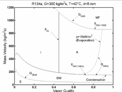
The flow pattern map for evaporation is shown in Figure 1 for R-134a in an 8.0 mm tube evaluated at 40°C. The transition boundary between annular flow (A) and stratified-wavy (SW) flow at high vapor quality represents the onset of dryout of the annular film and is thus a function of heat flux. For condensation, saturated vapor enters a condenser tube and forms either a thin liquid film around the perimeter of the tube (as an annular flow) or a liquid layer in the bottom of the tube and a gravity-controlled condensing film around the upper perimeter (as a stratified or stratified-wavy flow). Since dryout does not actually occur for condensation, the transition curve labeled Gwavy is presumed to reach its minimum
value and then continue horizontally to the vapor quality of 1.0, as shown in Figure 1. This means that a saturated vapor enters at x = 1.0 and goes directly into either the annular flow regime, the stratified-wavy flow regime or the stratified regime, depending on whether G is greater or less that Gwavy or Gstrat. The other boundaries
regime occurs at mass velocities higher than those shown on the present map and is also beyond our current database. In a mist flow, it can be envisioned that the layer of condensate will be sheared from the wall and that a new condensate layer will immediately begin to grow again in its place.
Figure 1. Condensation flow pattern map boundaries compared to evaporation map boundaries.
To cover a broader range of reduced pressures from 0.02 to 0.80, the second change to the condensation map relative to the prior evaporation map is its method for calculating void fraction, where a simple logarithmic mean void fraction ε is introduced and calculated as
(
h ra)
ra h
ε ε
ε ε ε
ln
−
= (4)
In this expression, the value of εra from the Rouhani and
Axelsson [10] drift flux expression:
( )
[
]
( ) (
[
)
]
1
5 . 0
25 . 0
1 18 . 1
1 1
12 . 0 1
−
− −
+
−
+ −
+ =
L V L
L V V
ra
G g x
x x x x
ρ ρ ρ σ
ρ ρ ρ
ε (5)
and the homogeneous void fraction εh is calculated as:
1
1 1
−
− + =
L V h
x x
ρ ρ
ε (6)
For the complete set of equations for the condensation flow pattern map, refer to El Hajal, Thome and Cavallini [2]. Figure 2 depicts a comparison of this map to flow pattern observations for R-407C obtained by Liebenberg, Thome and Meyer [3], in which all observations at the test conditions indicated were correctly identified.
0 200 400 600 800 1000
0 0.2 0.4 0.6 0.8 1
VAPOUR QUALITY, (-)
M
A
S
S
F
L
U
X
,
(k
g
/m
2s
)
G = 300 kg/m^2s
G = 400 kg/m^2s
G = 500kg/m^2s
G = 600 kg/m^2s
G = 700 kg/m^2s
G = 800 kg/m^2s
INTERM IT TEN T A NN ULA R
ST RA TIF IED & WAVY
T R A N S I T I O N
Figure 2. Flow pattern observations for R-407C compared to condensation flow pattern map.
Heat Transfer Model for Pure Vapors and Azeotropic Mixtures
The objective here was to develop a new flow pattern/flow structure based condensation heat transfer model analogous to that proposed by Kattan, Thome and Favrat [11] for evaporation inside horizontal tubes. The condensation heat transfer model proposed by Thome, El Hajal and Cavallini [4] uses the same flow pattern map as for evaporation but with the new modifications noted above. The new condensation model assumes that two types of heat transfer occur around the perimeter of the tube: convective condensation and film condensation. Convective condensation refers to the axial flow of the condensate along the channel due to the imposed pressure gradient while film condensation refers to the flow of condensate from the top of the tube towards the bottom due to gravity. Previous condensation models typically have subdivided the process into only two flow regimes: stratified flow and unstratified flow. Instead, here it is divided into the traditional flow regimes: annular flow, stratified-wavy flow, fully stratified flow, intermittent flow, mist flow and bubbly flow. Only the first five are addressed here as few data are available for bubbly flows while intermittent and mist flows are treated as an annular flow for simplicity’s sake. The three basic two-phase flow structures assumed are shown in Figure 3.
Figure 3. Flow structures for annular, stratified-wavy and fully stratified flows (left to right in bottom three diagrams) and for fully stratified flow and its film flow equivalent (top two diagrams).
Figure 4. Heat transfer zones on perimeter of tube in stratified types of flows.
The above two heat transfer mechanisms are applied to their respective heat transfer surface areas as shown in Figure 4. The convective condensation heat transfer coefficient αc is applied to the
perimeter wetted by the axial flow of liquid film, which refers to the entire perimeter in annular, intermittent and mist flows but only part of the perimeter in stratified-wavy and fully stratified flows. The axial film flow is assumed to be turbulent. The film condensation heat transfer coefficient αf is applied to the perimeter that would
upper perimeter of the tube for stratified-wavy and fully stratified flows. αf is obtained by applying the Nusselt [12] falling film theory
to the inside of the horizontal tube, which assumes the falling film is laminar and falls downward without any axial velocity component. Heat transfer coefficients for stratified types of flow are known experimentally to be a function of the wall temperature difference and this effect is included through the Nusselt falling film heat transfer equation in the present model.
The general expression for the local condensing heat transfer coefficient αtp is:
(
)
r r r c f tp π α θ π θ α α 2 2 − + = (7)In this expression, r is the internal radius of the tube and θ is the falling film angle around the top perimeter of the tube, which occurs on the upper perimeter that would otherwise be dry in an adiabatic stratified flow. Hence, for annular flow with θ = 0, αtp is equal to αc.
The falling film angle is obtained as follows. First, the stratified angle θstrat is calculated from the following implicit geometric
equation:
(
)
(
)
[
strat strat]
L
d
A = 2π−θ −sin2π−θ 8
2
(8)
where the cross-sectional area occupied by the liquid phase AL is
( )
AAL= 1−ε (9)
and the cross-sectional area occupied by the vapor is
AV =εA=1−AL (10)
A is the total cross-sectional area of the tube and ε is the local vapor void fraction, which is determined using the logarithmic mean void fraction (LMε) using the Rouhani and Axelsson drift flux model and the homogeneous model in order to cover the range from low to high reduced pressures.
For annular, intermittent and mist flows, θ = 0. For fully stratified flow, θ = θstrat. For stratified-wavy flow, the stratified
angle θ is obtained by assuming a quadratic interpolation between its maximum value of θstrat at Gstrat and its minimum value of 0 at
Gwavy:
(
)
(
)
5 . 0 − − = strat wavy wavy strat G G G G θ θ (11)The values of Gstrat and Gwavy at the vapor quality in question are
determined from their respective transition equations in the flow pattern map.
The convective condensation heat transfer coefficient αc is
obtained from the following turbulent film equation:
i L m L n L
c c δ f
λ
α = Re Pr (12)
where the liquid film Reynolds number ReL is based on the mean
liquid velocity of the liquid in AL as:
( )
( )
LL x G µ ε δ − − = 1 1 4 Re (13)
and PrL is the liquid Prandtl number defined as:
L L pL L c λ µ = Pr (14)
In these expressions c, n and m are empirical constants determined from the heat transfer database and δ is the thickness of the liquid film. The best value of the exponent m on PrL was
determined to be m = 0.5 while the best values of c and n for Eq. (12) were found statistically to be c = 0.003 and n = 0.74. The liquid film thickness δ is obtained from solving the following geometrical expression:
(
)
[
2(
2)
2]
8
2π−θ − − δ
= d d
AL (15)
where d is the internal diameter of the tube. When the liquid occupies more the one-half of the cross-section of the tube in a stratified-wavy or fully stratified flow at low vapor quality, this expression will yield a value of δ > d/2, which is not geometrically realistic. Hence, whenever δ > d/2, δ is set equal to d/2.
Analysis of the data demonstrated that an additional factor influenced convective condensation. After looking at various possibilities, the interfacial surface roughness was identified as the most influential based on the following reasoning. First of all, the shear of the high speed vapor is transmitted to the liquid film across the interface and hence increases the magnitude and number of the waves generated at the interface, which in turn increases the available surface area for condensation, tending to increase heat transfer. Secondly, the interfacial waves are non-sinusoidal and thus tend to reduce the mean thickness of the film, again increasing heat transfer. An interfacial roughness correction factor fi was introduced
to act on αc in Eq. (12) as follows:
(
)
1/42 2
/ 1
1
− + = σ δ ρ ρ g u u
f L V
L V
i (16)
where uV and uL are the mean velocities of the phases in their
respective cross-sectional areas AV and AL:
( )
( )
ερ − − = 1 1 L L x G u (17) ε ρV V Gx
u = (18)
The interfacial roughness correction factor fi tends towards a
value of 1.0 as the film becomes very thin (roughness must be proportional to film thickness) but fi tends to increase as the slip
ratio uV/uL increases. Finally, fi tends to decrease as σ increases,
since surface tension acts to smooth out the waves. For fully stratified flow, interfacial waves are damped out and hence the above expression becomes
(
)
− + = strat V L L V i G G g u u f 4 / 1 2 2 / 1 1 σ δ ρ ρ (19)when G < Gstrat, which produces a smooth variation in αtp across this
flow pattern transition boundary just like for all the other transition boundaries and the ratio of G/Gstrat acts to damp out the effect of
The film condensation heat transfer coefficient αf is obtained
from the theory of Nusselt [12] for laminar flow of a falling film on the internal perimeter of the tube, where αf is the mean coefficient
for this perimeter. Rather than integrating from the top of the tube to the stratified liquid layer at θ/2 to obtain αf, which would be more
theoretically satisfying, it was found sufficient to simply use the mean value for condensation around the perimeter from top to bottom with its analytical value of 0.728, and thus avoid a numerical integration to facilitate practical use of this method in designing condensers. Hence, αf is:
(
)
(
)
4 1
w sat L
3 L LV V L L f
T T d
λ
h g
ρ
ρ
ρ
0.728
α
− −
= (20)
Since heat exchanger design codes are typically implemented assuming a heat flux in each incremental zone along the exchanger, it is more convenient to convert this expression to heat flux using Newton’s law of cooling, such that the heat flux version of the Nusselt equation where the local heat flux is q, is given by the expression:
(
)
31
L
3 L LV V L L f
q d
λ
h g
ρ
ρ
ρ
0.655
α
−
= (21)
where the leading constant 0.655 comes from 0.7284/3. The difference in the accuracy of the predictions whether using the first or second of these expressions for αf is negligible.
To completely avoid any iterative calculations, the following
expression of Biberg [13] based on void fraction is used to very accurately (error ≈ 0.00005 radians for 2π≥θstrat≥ 0) evaluate θstrat
instead of Eq. (8):
( )
( )
( )
( )
[
( )
]
( )
(
)
[
]
+ − +
− − − −
− −
+ − −
+ −
− =
2 2
3 / 1 3 / 1
3 / 1
1 4 1
1 2 1 1 200
1 1
1 2 1
2 3 1
2 2
ε ε
ε ε
ε ε ε
ε π ε π
π
θstrat (22)
The above heat transfer prediction method cannot be evaluated at ε = 1.0 because of division by zero. Furthermore, experimental condensation heat transfer test data are reported with a measured error in vapor quality of at least ±0.01 and hence it does not make sense that test data can be evaluated for x > 0.99. Thus, the above condensation prediction method is applicable when 0.99 ≥ x; when x > 0.99, then x should be reset to 0.99. Also, the lower limit of applicability is for vapor qualities x ≥ 0.01. Our range of test data was from 0.97 > x > 0.03. This method provides for a smooth variation in αtp across all the flow pattern transition boundaries
without any jump in the value of αtp.
The condensation heat transfer model is implemented as follows:
1. Determine the local vapor void fraction using the LMε method given by Eq. (6);
2. Determine the local flow pattern using the flow pattern map; 3. Identify the type of flow pattern (annular, intermittent, mist,
stratified-wavy or stratified);
4. If the flow is annular or intermittent or mist, then θ = 0 and
αc is determined with Eq. (12) and hence αtp = αc in Eq. (7)
where δ is obtained with Eq. (15) and fi is determined with
Eq. (16).
5. If the flow is stratified-wavy, then θstrat and θ are calculated
using Eq. (8) or (22) and Eq. (11), then αc and αf are
calculated using Eqs. (12) and (20) or (21), and finally αtp is
determined using Eq. (7) where again δ is obtained with Eq. (15) and fi is determined with Eq. (16).
6. If the flow is fully stratified, then θstrat is calculated using
Eq. (8) or (22) and θstrat is set equal to θ, then αc and αf are
calculated using Eqs. (12) and (20) or (21), and finally αtp is
determined using Eq. (7) where δ is obtained with Eq. (15) and fi is determined with Eq. (19).
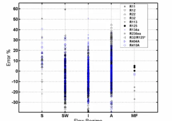
Figure 5 depicts a comparison of the new condensation heat transfer model to all the refrigerant database, representing eleven fluids with a total of 1850 data points taken by nine different research laboratories. Based on all the data points from these numerous different test facilities, 85% are predicted within ±20%. Figure 6 depicts the distribution of errors by flow pattern, showing nearly uniform accuracy except for the fully stratified flows (where heat transfer is dominated by Nusselt film condensation and whose perimeter-averaged heat transfer coefficient may not be well represented by the measurement techniques).
Figure 5. Comparison of condensation heat transfer model to entire refrigerant database.
Figure 6. Comparison of condensation heat transfer model to entire refrigerant database by flow pattern.
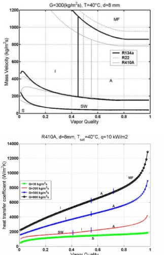
To illustrate the predicted trends in αtp as a function of vapor
diameter tube assuming a heat flux of 40 kW/m2. The flow pattern map (for three refrigerants) and heat transfer coefficients (for R-410A) are shown in Figure 7. At the lowest flow rate, 30 kg/m2s, the flow is in the stratified regime from inlet to outlet and the heat transfer coefficient falls off slowly with decreasing vapor quality. At 200 kg/m2s, the flow enters in annular flow and then passes through
intermittent and stratified-wavy flow. At 500 kg/m2s, the flow enters in the annular flow regime and converts to intermittent flow at about x = 0.55 and leaves in this same regime. The sharp decline in αtp at
high vapor qualities results from the rapid growth of the annular film thickness. At 800 kg/m2s, the flow enters in the mist flow regime, goes into the annular flow regime and then leaves in the intermittent regime. As can be seen, the new heat transfer model predicts the variation in the local heat transfer coefficients across flow pattern transition boundaries without any discontinuity in the value of αtp.
Figure 7. Simulation of flow pattern map and heat transfer model for condensation of R-410A.
Heat Transfer Model for Zeotropic Mixtures
The mixture effect on condensation heat transfer is illustrated by Figure 8 showing local experimental heat transfer coefficients for three refrigerant mixtures of R-125/R-236ea and its pure components obtained by Cavallini et al. [14]. Applying the new version of the Silver [15] and Bell and Ghaly [16] method by Del Col, Cavallini and Thome [5], the local heat transfer coefficient for zeotropic mixtures αtpm is obtained from the film condensation
coefficient αfm and the convective condensation coefficient αcm by
accounting for the different perimeters pertaining to the two mechanisms:
0 500 1000 1500 2000 2500 3000 3500 4000 4500 5000
0 0.2 0.4 0.6 0.8 1
MASS COMPOSITION (fraction of R-125)
H
E
A
T
T
R
A
N
S
F
E
R
C
O
E
F
F
IC
IE
N
T
[W
/(
m
2 K
)] x = 0.3 Tsat = 47°C
x = 0.5 Tsat = 51°C
x = 0.7 Tsat = 54°C
G = 400 kg/(m2 s)
Figure 8. Heat transfer coefficients for three refrigerant mixtures of R-125/R-236ea and its pure components obtained by Cavallini et al. [14].
(
)
r r
r cm
fm
tpm π
α θ π θ α α
2
2 −
+
= (23)
where θ is the falling film angle around the top perimeter of the tube as already discussed. The convective condensation heat transfer coefficient of the mixture is obtained from the Silver-Bell-Ghaly series resistance approach as follows:
1
1 −
+
= c
c
cm α R
α (24)
where αc is computed as per the pure fluid model using mixture
physical properties. The Silver-Bell-Ghaly vapor-phase heat transfer resistance Rc for cooling of the vapor to the dew point temperature
is calculated as follows:
Vi m gl pV c
h T c x R
α
∆
∆
1= (25)
The resistance depends on vapor phase heat transfer coefficient referred to the vapor-liquid interface αVi. Silver-Bell-Ghaly assumed
the value of αVi to be that of simple vapor flow in a plain tube
without a liquid film while in fact there is a liquid film with an interfacial roughness affecting this heat transfer. Based on this reasoning, the same correction factor acting on αc should be applied
to the vapor heat transfer coefficient that appears in the Silver-Bell-Ghaly resistance of the axial flow. Therefore the vapor coefficient can be written as:
i V Vi α f
α = (26)
The interfacial roughness factor fi is computed from the
equations above. The vapor heat transfer coefficient αV can be
computed with the Dittus and Boelter [17] correlation:
33 . 0 8 .
0 Pr
Re 023 .
0 V V
V V
d λ
It is adapted to the present situation by defining the Reynolds number of the vapor phase ReV based on the mean vapor velocity of
the cross-sectional area occupied by the vapor AV:
V V
Gdx εµ =
Re (28)
PrV is the vapor Prandtl number. The Silver-Bell-Ghaly
procedure is applied to the film condensation component in the same way as for the convective term but without interfacial roughness on the laminar falling film, i.e. fi = 1.0. One of the main
assumptions of the Silver-Bell-Ghaly approach is that equilibrium exists between the liquid and vapor phases. In reality, the condensation process inside a tube departs from this equilibrium when the liquid condensate forms a stratified layer at the bottom of the tube and the film condensation component must be further corrected with a mixture factor Fm acting to the resistance of the
falling film:
1
1 −
+ ⋅
= f
f m
fm F α R
α (29)
The heat transfer coefficient αf is calculated from the pure vapor
model using the properties of the mixture while the resistance Rf can
be determined in the form:
V m gl pV f
h T c x R
α
1
∆ ∆ ⋅
= (30)
where no interfacial roughness factor applies to the vapor phase heat transfer coefficient because the falling film is supposed to be smooth. The new non-equilibrium mixture factor Fm accounts for
non-equilibrium effects in stratified flow regimes and has been correlated as a function of vapor quality, mass velocity, temperature glide and saturation to wall temperature difference as follows:
−
⋅ − ⋅ − =
w sat
gl 0.5 wavy m
T T
T
G G x) (1 0.25 exp
F (31)
The values of Fm range between 0 and 1. It decreases when
stratification is enhanced, that is at low mass velocity and low vapor quality. The mass transfer resistance depends on the temperature glide and that is why Fm decreases when increasing ∆Tgl. Finally,
the effect of the saturation to wall temperature difference is the opposite of that in the Nusselt theory. Given the saturation temperature, when the wall temperature decreases, the vapor of the more volatile component accumulates near the interface and acts as an incondensable. When this temperature difference increases, the more volatile component begins to condense and this decreases the thermal resistance of the diffusion layer. This is the reason why the factor Fm should increase with the saturation to wall temperature
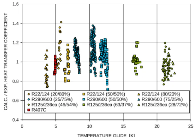
difference, leading to an increase in the heat transfer coefficient. Figure 9 depicts the comparison of this method to test data from four publications. The database covers temperature glides up to 22 K and mass velocities from 57-755 kg/m2s. The method predicts 98% of the refrigerant heat transfer coefficients measured by Cavallini et al. [14, 18] to within ±20% and predicts 85% of the halogenated plus hydrocarbon refrigerant heat transfer coefficients measured by Lee [19] and Kim, Chang and Ro [20] to within ±20%.
0.4 0.6 0.8 1 1.2 1.4 1.6
0 5 10 15 20 25
TEMPERATURE GLIDE [K]
C
A
L
C
.
/
E
X
P
.
H
E
A
T
T
R
A
N
S
F
E
R
C
O
E
F
F
IC
IE
N
T
R22/124 (20/80%) R22/124 (50/50%) R22/124 (80/20%) R290/600 (25/75%) R290/600 (50/50%) R290/600 (75/25%) R125/236ea (46/54%) R125/236ea (63/37%) R125/236ea (28/72%) R407C
Figure 9. Comparison of new mixture model to complete database plotted versus the mixture temperature glide.
Summary
Recent improvements in general thermal design methods for condensation inside plain, horizontal tubes made at the Laboratory of Heat and Mass Transfer at the EPFL in collaboration with the University of Padova and the University of Pretoria have been summarized. First, a new condensation two-phase flow pattern map has been proposed and partially verified by new flow pattern observations. Secondly, a new condensation heat transfer model has been developed including both flow pattern effects and interfacial roughness effects, which accurately predicts and emulates a large, diversified database. Finally, the well-known Silver-Bell-Ghaly model for predicting heat transfer in the condensation of miscible vapor mixtures has been adapted to this new heat transfer model, including the effects of interfacial flow structure and roughness on vapor phase heat transfer and non-equilibrium condensation, to more accurately predict condensation of mixtures with temperature glides up to 22 K.
References
Smit, F.J., Thome, J.R. and Meyer, J.P. (2002). Heat Transfer Coefficients during Condensation of the Zeotropic Mixture R-22/R-142b, J.
Heat Transfer, 124, 1137-1146.
El Hajal, J., Thome, J.R., and Cavallini, A. (2003). Condensation in Horizontal Tubes, Part 1: Two-Phase Flow Pattern Map, Int. J. Heat Mass
Transfer, vol. 46, 3349-3363.
Liebenberg, L., Thome, J.R. and Meyer, J.P. (2004). Flow Pattern Identification with Power Spectral Density Distributions of Pressure Traces during Refrigerant Condensation in Smooth and Micro-Fin Tubes, J. Heat
Transfer, in review.
Thome, J.R., El Hajal, J. and Cavallini, A. (2003). Condensation in Horizontal Tubes, Part 2: New Heat Transfer Model Based on Flow Regimes, Int. J. Heat Mass Transfer, 46, 3365-3387.
Del Col, D., Cavallini, A. and Thome, J.R. (2004). Condensation of Zeotropic Mixtures in Horizontal Tubes: New Simplified Heat Transfer Model Based on Flow Regimes, J. Heat Transfer, in review.
Akers, W.W., Deans, H.A., and Crosser, O.K. (1959). Condensation Heat Transfer within Horizontal Tubes, Chem. Eng. Prog. Symp. Ser., 55, 171-176.
Kattan, N., Thome, J. R., and Favrat, D. (1998). Flow Boiling in Horizontal Tubes. Part 1: Development of a Diabatic Two-Phase Flow Pattern Map, J. Heat Transfer, 120, 140-147.
Thome, J.R., and El Hajal, J. (2002). Two-Phase Flow Pattern Map for Evaporation in Horizontal Tubes: Latest Version, 1st Int. Conf. On Heat
Transfer, Fluid Mechanics and Thermodynamics, Kruger Park, South Africa,
April 8-10, 1, 182-188.
Collier, J.G., and Thome, J.R. (1994). Convective Boiling and
Rouhani, Z., and Axelsson, E. (1970). Calculation of Volume Void Fraction in the Subcooled and Quality Region, Int. J. Heat Mass Transfer, 13, 383-393.
Kattan, N., Thome, J. R., and Favrat, D. (1998). Flow Boiling in Horizontal Tubes. Part 3: Development of a New Heat Transfer Model Based on Flow Patterns, J. Heat Transfer, 120, 156-165.
Nusselt, W. (1916). Die oberflachenkondensation des wasser-dampfes,
Z. Ver. Dt. Ing., 60, 541-546 and 569-575.
D. Biberg (1999). An Explicit Approximation for the Wetted Angle in Two-Phase Stratified Pipe Flow, Canadian J. Chemical Engineering, 77, 1221-1224.
Cavallini, A., Censi, G., Del Col, D., Doretti, L., Longo, G.A., Rossetto, L., Zilio, C. (2000). Analysis and Prediction of Condensation Heat Transfer of the Zeotropic Mixture R-125/236ea, Proc. of the ASME Heat Transfer
Division, HTD- 366-4, 103-110.
Silver, L. (1947). Gas Cooling with Aqueous Condensation, Trans. Inst.
Chem. Eng, 25, 30-42.
Bell K.J., Ghaly M.A. (1973). An Approximate Generalized Design Method for Multicomponent/Partial Condenser, AIChE Symp. Ser., 69, 72-79.
Dittus, F.W., Boelter, M.L.K. (1930). Heat transfer in automobile radiators of the tubular type, University of California Publications on Engineering, Berkeley, CA 2(13), 443.
Cavallini, A., Del Col, D., Doretti, L., Longo, G.A., Rossetto, L. (1999). Condensation of R-22 and R-407C inside a Horizontal Tube, Proc. of 20th
Int. Congress of Refrigeration, IIR/IIF, Sydney.
Lee, Chung-Chiang (1994). Investigation of Condensation Heat Transfer of R124/22 Nonazeotropic Refrigerant Mixtures in Horizontal Tubes, National Chiao Tung University, Taiwan, Ph.D. Thesis.